Working
Paper
361
The finite-sample size of the BDS
test for GARCH standardized
residuals
Marcelo Fernandes
Pierre-Yves Preumont
CEQEF - Nº18
W
ORKINGP
APER361
–
CEQEF
Nº18
•
Maio
DE2014
•
1
Os artigos dos
Textos para Discussão da Escola de Economia de São Paulo da Fundação Getulio
Vargas
são de inteira responsabilidade dos autores e não refletem necessariamente a opinião da
FGV-EESP. É permitida a reprodução total ou parcial dos artigos, desde que creditada a fonte.
Escola de Economia de São Paulo da Fundação Getulio Vargas FGV-EESP
for GARCH Standardized Residuals
Marcelo Fernandes** Pierre-Yves Preumont***
Abstract
This paper uses a multivariate response surface methodology to analyze the size distortion of the BDS test when applied to standardized residuals of first-order GARCH processes. The results show that the asymptotic standard normal distribution is an unreliable ap-proximation, even in large samples. On the other hand, a simple log-transformation of the squared standardized residuals seems to correct most of the size problems. Nonethe-less, the estimated response surfaces can provide not only a measure of the size distortion, but also more adequate critical values for the BDS test in small samples.
Keywords: BDS Test, GARCH Process, Response Surface, Size Distortion.
JEL Codes: C15, C52.
*
Submitted in ??. Revised in ??. We wish to thank the anonymous referee and many seminar participants for their helpful comments. The usual disclaimer applies.
**
S˜ao Paulo School of Economics, Funda¸c˜ao Getulio Vargas, Brazil. E-mail: marcelo. [email protected]
***
1. Introduction
The extensive literature on GARCH-type processes is clearly a consequence of their success in modeling financial time series. This class of models is specifi-cally designed to handle volatility clustering and leptokurtosis. Furthermore, it is possible to interpret GARCH models as discrete approximations of jump-diffusion processes Nelson (1990a), Drost and Werker (1996). On the other hand, some papers present evidence that GARCH models are not able to fully explain all nonlinear dependence in financial data (e.g. Hsieh, 1991, Peel and Speight, 1994, Abhyankar et al., 1995).
A common procedure is to apply the BDS test described in Brock et al. (1996) to the standardized residuals of GARCH models. The BDS test has good power against a wide class of data generating processes that depart from the property of independence and identical distribution (iid). Moreover, the BDS test does not require the existence of high-order moments, as opposed to most alternative tests that usually assume the existence of the fourth or even higher moments de Lima (1997). Since financial data does not often satisfy these requirements, the robustness of the BDS test to failure of moment conditions is a particularly desirable property.
However, pre-filtering the data using a GARCH-type process distorts the asymptotic distribution of the BDS statistic as a consequence of the nonzero variance of the estimates (see Brooks and Heravi, 1999). There are some solu-tions in the literature. Brock et al. (1991) perform Monte Carlo simulasolu-tions to derive the distribution of the BDS test on standardized residuals stemming from a specific GARCH(1,1) model. Hsieh (1993) uses the same procedure to determine proper critical values for the BDS test when applied to standardized residuals of EGARCH and autoregressive volatility models. Chappell et al. (1996) and Fer-nandes (1998) bootstrap the standardized residuals of conditional heteroskedastic models for exchange rate series to illustrate the degree of size distortion. Finally, de Lima (1996) proves the nuisance parameter free property of the BDS test for ad-ditive models, which requires working with the logarithm of the squared GARCH standardized residuals as in Brock and Potter (1992). Taking the squares of the standardized residuals dooms the BDS test to have no power against alternatives featuring asymmetry, such as the leverage effect singled out by Black (1976).
The results confirm that, in finite samples, the selection of the embedding di-mension for the BDS test plays a role in the size distortion. This occurs, even though the distribution of the test should be, under the null hypothesis, the same regardless of the dimension. One novel piece of evidence is the significant rela-tionship between the persistence in volatility and the nuisance parameter effect. Finally, the results for the logarithm of the squared standardized residuals are en-couraging, since it seems to correct, even in moderate sample sizes, the distortions due to the presence of nuisance parameters.
The paper is organized as follows. Section 2 discusses in detail the BDS test and its properties. Section 3 outlines the response surface methodology for determining the size bias implied by the asymptotic distribution of the BDS test in the presence of nuisance parameters. Section 4 compares the results of the response surface estimation for the cases of standardized residuals and of transformed residuals. Section 5 uses an empirical example to illustrate how the results of the test can qualitatively change if one considers more precise critical values, such as those provided by the surface response. Section 5 offers some concluding remarks.
2. A Closer Look at the BDS Test
The nonparametric test of Brock et al. (1996) is derived from the correlation integral, which is a measure of the spatial correlation between scattered points in the m-dimensional space. In a time-series context, {xt} is embedded in the
m-space by forming m-histories xm
t = (xt, xt−1, . . . , xt−m+1). The correlation
integral reads
C(δ, m) = Z
u
Z
v
I(u, v, δ)dFm(u)dFm(v),
where the indicator kernel functionI(·) is one if |u−v|< δ, zero otherwise, and
Fm(·) is the distribution function ofxmt . Hence, it indicates the concentration of
the joint distribution ofm-consecutive observations.
Brock et al. (1996) have shown that the generalized U-statistic
C(δ, m, T) = 2
(T−m)(T−m+ 1) X
t<s
I(xmt , xms, δ)
is a consistent estimator ofC(δ, m) provided that{xt}is an absolutely regular and
strictly stationary stochastic process. The fact that C(δ, m, T) is an U-statistic entails some interesting properties. For instance, under certain conditions, U-statistics are minimum variance estimators in the class of all unbiased estimators and converge rapidly to normality Serfling (1980).
If the process {xt} is iid, then Fm(xmt ) =
Qm−1
i=0 F1(xt−i), and C(δ, m) =
C(δ,1)m almost surely. Brock et al. (1996) use this relation to construct the
BDS(δ, m, T) =√T C(δ, m, T)−C(δ,1, T)
m
σ(δ, m, T) ,
whereσ(δ, m, T) is a nontrivial function of the correlation integral. Strong consis-tency and asymptotically standard normality are proven using U-statistic theory. Moreover, the BDS test has high power against a vast class of linear, nonlinear, and nonstationary models.
The asymptotic distribution of the BDS statistic is also invariant to the esti-mation process of smooth filters under some modest conditions de Lima (1996). In particular, the process {xt} must be strong mixing, with mixing coefficients satisfying the summability condition P∞
k=1α 1/2
k <∞, and the filter must be an
additive noise model Tong (1990) with parameters√T-consistently estimated. Al-though the GARCH(p, q) model
yt=
p
htǫt, ǫt∼iid(0,1), ht=ω+ p
X
i=1
αiyt2−i+ q
X
j=1
βjht−j
is multiplicative, it is readily converted into an additive noise model. Brock and Potter (1992) and de Lima (1996) indeed suggest transforming the standardized residuals as follows
ηt≡logǫ2t = logyt2−loght.
Under the null hypothesis of correct specification, the standardized error ǫt
is iid, which implies that ηt is also iid. In addition, the parametric restrictions
normally imposed to achieve covariance stationarity and positivity of the condi-tional variance suffice to guarantee the invariance property de Lima (1996), since the parameters can be√T-consistently estimated by pseudo-maximum likelihood Bollerslev and Wooldridge (1992).
3. A Response Surface Analysis
In this section, we describe the experimental design using Hendry’s (1984) terminology. The data generating process is a GARCH(1,1) model with normal conditional distribution, viz.
yt=
p
htǫt, ǫt|It−1∼N(0,1), ht=ω+αy2t−1+βht−1.
The Monte Carlo design variables are the parametersθ, the embedding dimen-sionm, and the sample sizeT, where
θ= (ω, α, β)′
∈Θ ={θ|ω >0, α >0, β >0, α+β <1},
m ∈ M= [ m, m], and T ∈ T = T , T . An underline indicates the smallest value, whereas an overline corresponds to the largest value we consider for any given variable. The parameter space thus is Θ× M × T. The relationship of interest for the BDS statistic is the correct null hypothesis{H0 :ǫt is iid}, so as
to address the size of the test. The aim of the simulation exercise is to investigate the deterioration of the asymptotic distribution of the BDS test when applied to the standardized residuals. The nuisance parameter bias presumably depends uponθ,m, andT, implying that we must pursue an adequate approximation over
Θ× M × T.
We hold two parameters constant across experiments: ω and δ. There is no loss of generality settingωto one, for it is only a scale factor. By the same token, the actual standard deviation ofǫt is assigned to the tuning parameterδso as to
optimize the power and size of the test Brock et al. (1991). Therefore,δ= 1 when the test is applied to the standardized residuals andδ= 2.22 when applied to the transformed residuals. The values of the GARCH parameters cover a large range of processes:
(α, β)∈ {α∈Θ∗, β∈Θ∗|α+β <1},
where Θ∗={0.1,0.2,0.3,0.4,0.5,0.6,0.7,0.8}. We also compute the BDS statistic
for several embedding dimensions: m ∈ {2,3,4,5,6,7,8}. Albeit we investigate four sample sizes, withT ∈ {100,250,500,1000}, we keep the number of replica-tions constant atN = 1,000 for all experiments. Given the selection of the key parameters and the covariance stationarity constraint (α+β < 1),1 we adopt a full factorial design, totaling 1,008 experiments.
We draw 5,000 standard normal variates to generate each GARCH process, but we use only the lastT observations for estimation purposes to avoid any spurious effect due to the initial conditions. Furthermore, we seth0 to the unconditional variance, that is to say,h0=ω/(1−α−β). The estimation ofθis by maximum
1
likelihood. We the compute the BDS statistic for both the standardized residuals ˆ
ǫtand the transformed residuals ˆηt.
We gauge the size distortion for the lower and upper tail of the distribution, since one usually performs the BDS test considering both tails. More precisely, we compute the ratio between the critical values CVα derived from the Monte
Carlo simulations and the α-quantiles CV∞
α of the asymptotic standard normal
distribution, whereα∈ {0.025,0.050,0.950,0.975}. The absence of size distortion would then implyDα≡CVα/CVα∞ equal to one for everyα.
As the exact functional form is unknown, we adopt the usual power-series approximation for the response surface analysis. More precisely, we start with three initial specifications forD=Q(θ, Tm) +υ, namely
Q1(θ, Tm) = g(α, β,1/Tm)
Q2(θ, Tm) = g(α+β,1/Tm)
Q3(θ, Tm) = g(1/Tm)
whereTmis the effective sample size adjusted by the embedding dimension,2 υis
a white noise vector, and g(·) denotes a polynomial of second order. In contrast to the first approximation Q1 that sets the size distortion as a function of the individual values of the parameters, Q2 assumes that the implied persistence in volatility summarizes all the information in the parameters. Finally,Q3 suggests that the level distortion is solely due to finite sample sizes.
The estimation is by SUR so as to account for the correlation among the errors of each equation. We use a training subsample of 800 (randomly chosen) experiments for estimation purposes, while keeping the remaining 208 experiments to assess the validity and precision of the different approximations through out-of-sample analysis. Therefore, the model selection procedure contains two stages: in-sample and out-of-sample. In the training set, for each starting functional form (Q1,Q2, andQ3), we adopt a general-to-specific approach to find the more adequate approximation. We consecutively delete the less significant parameter of the system until all coefficients are statistically different from zero at the 5% level of significance. We then compare the in-sample and out-of-sample performance of the resulting systems of each starting specification.
4. Modeling the Size Distortion
In this section, we report the outcome of the model selection procedure and discuss the estimation results of the response surface systems, comparing the best
2
In theory, the embedding dimension does not play any role, other than reducing the ef-fective sample size available to compute the correlation integral. We consider two measures of adjusted sample size: T −m+ 1 andT /m. The former corresponds to the total number of
representations for the cases of standardized and transformed residuals. In partic-ular, we show some evidence that the nuisance parameter effect on the distribution of the BDS test increases with the persistence in volatility. On the other hand, for the case of the transformed residuals, the size bias depends only upon the effective sample size and the test statistic seems to converge in distribution to a standard normal.
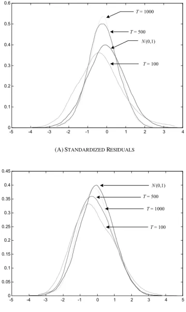
Before discussing in detail the selection and estimation of the response surfaces, it is important to observe some features of the BDS test distribution for both stan-dardized and transformed residuals. Figure 1 exhibits the estimated distributions of the test for both cases to highlight their differences in a relatively large sample. Figure 2 plots the nonparametric estimation for the distribution of the test when applied to the standardized (Figure 2a) and transformed residuals (Figure 2b), stressing the effects of sample size.3 As the sample size increases, the distributions in Figure 2b become closer to the normal distribution, which is clearly not the case in Figure 2a. Indeed, despite the high skewness, the distribution of the BDS statistic in Figure 2a is more similar to the standard normal whenT = 100. This peculiarity is probably a consequence of the interaction of two opposite forces: the finite sample bias and the nuisance parameter effect.
Figure 1
The distribution of the BDS test (m= 4, α= 0.1, β= 0,8, T = 1000)
-5 -4 -3 -2 -1 0 1 2 3 4 0
0.1 0.2 0.3 0.4 0.5 0.6
standardized
residuals
N(0,1)
Figure 1 – The distribution of the BDS test (m = 4, α = 0.1, β = 0.8, T = 1000)
transformed
residuals
3
Figure 2
The distribution of the BDS test in finite samples (m= 4, α= 0.1, β= 0,8)
-5 -4 -3 -2 -1 0 1 2 3 4 0
0.1 0.2 0.3 0.4 0.5 0.6
-5 -4 -3 -2 -1 0 1 2 3 4 5 0
0.05 0.1 0.15 0.2 0.25 0.3 0.35 0.4 0.45
T = 1000
T = 500
N (0,1)
T = 100
N (0,1)
T = 1000 T = 500
T = 100
(A)STANDARDIZED RESIDUALS
(B)TRANSFORMED RESIDUALS
Table 1 reports the average effective size of the BDS test over the different sets of GARCH parameters, according to the sample size and the embedding dimension. In small samples (100 observations), the lack of precision in the estimation of the GARCH parameters and of the correlation integral causes over-rejection of the correct null hypothesis on both standardized and transformed residuals. As the sample size increases, the BDS test for the standardized residuals becomes more and more conservative, while the size distortion correction provided by the transformation of the residuals improves.
Tables 2 and 3 document the in-sample and out-of-sample performances of each specification, respectively. We assess the out-of-sample performance using two different metrics, namely the Euclidean norm and the norm of the maxi-mum, to gauge how large, on average, are the residual vectors of the multivariate response surfaces. For the standardized residuals, using the number of nonoverlap-pingm-histories to gauge the effective sample size dominates both in-sample and out-of-sample irrespective of the specification. The approximation based on the persistence in volatility, Q∗
2(θ, Tm), provides a marginally superior out-of-sample
fit. The fitted values are
b
D0.975 = 0.51 + 13.1m/T+ 51.6 (m/T)2+ 7.6 (α+β)m/T
−117.7 (α+β)(m/T)2+ 81.9 [(α+β)m/T]2 b
D0.950 = 0.49 + 12.4m/T+ 7.5 (α+β)m/T b
D0.050 = 0.52 + 36.3m/T−299.5 (m/T)2−56.3 (α+β)m/T +801.1 (α+β) (m/T)2+ 40.3 (α+β)2m/T
−612.0 [(α+β)m/T]2 b
D0.025 = 0.51 + 36.0m/T−317.2 (m/T)2−57.4 (α+β)m/T +855.7 (α+β) (m/T)2+ 41.7 (α+β)2m/T
−654.5 [(α+β)m/T]2.
The most striking feature is that the intercepts are remarkably distant from one, implying that the standard normal is not a good approximation for the test distribution, even asymptotically. Indeed, the asymptotic critical values corrected by the nuisance parameter effect are about half of the uncorrected ones provided by the standard normal distribution.
The shape of the response surfaces indicates that the size distortion is strongly dependent on the persistence in volatility only in small samples (see Figure 3). In the upper tail, the size bias linearly increases with the persistence in volatility (Figure 3a,b). In the lower tail, the size distortion is a nonlinear function of the degree of persistence and of the effective sample size (Figure 3c,d). Nevertheless, irrespective of the tail, the convergence towards the adjusted asymptotic critical values is rather fast.
Table 1
The average empirical size of the BDS test
standardized transformed sample dimension
5% 10% 5% 10%
T= 100 m= 2 0.08 0.13 0.10 0.17
m= 4 0.09 0.16 0.09 0.17
m= 6 0.14 0.22 0.10 0.17
m= 8 0.23 0.32 0.11 0.18
T= 250 m= 2 0.01 0.02 0.06 0.13
m= 4 0.01 0.03 0.06 0.12
m= 6 0.03 0.06 0.07 0.12
m= 8 0.06 0.11 0.07 0.13
T= 500 m= 2 0.00 0.01 0.06 0.12
m= 4 0.00 0.01 0.06 0.11
m= 6 0.01 0.02 0.06 0.11
m= 8 0.01 0.02 0.06 0.12
T= 1000 m= 2 0.00 0.01 0.05 0.11
m= 4 0.00 0.00 0.05 0.11
m= 6 0.00 0.01 0.04 0.10
m= 8 0.00 0.01 0.05 0.10
Table 2
In-sample performance of the response surface
D0.025 D0.050 D0.950 D0.975 approximation
R2
DW R2
DW R2
DW R2
DW
standardized residuals
Q∗
1(θ, T−m+ 1) 0.85 2.15 0.83 2.14 0.78 2.12 0.79 2.10
Q∗
1(θ, T /m) 0.92 1.91 0.93 1.93 0.96 1.95 0.96 1.91
Q∗
2(θ, T−m+ 1) 0.84 2.14 0.83 2.13 0.78 2.12 0.78 2.10
Q∗
2(θ, T /m) 0.92 1.84 0.92 1.88 0.95 1.95 0.95 1.92
Q∗
3(θ, T−m+ 1) 0.84 2.13 0.82 2.13 0.77 2.13 0.77 2.11
Q∗
3(θ, T /m) 0.91 1.82 0.91 1.87 0.94 2.01 0.94 1.99
transformed residuals
Q∗
1(θ, T−m+ 1) 0.57 1.98 0.66 2.07 0.67 2.07 0.64 2.08
Q∗
1(θ, T /m) 0.24 2.02 0.32 2.09 0.90 2.03 0.88 1.92
Q∗
2(θ, T−m+ 1) 0.56 1.98 0.65 2.05 0.67 2.06 0.64 2.08
Q∗
2(θ, T /m) 0.24 2.01 0.32 2.09 0.90 2.04 0.88 1.96
Q∗
3(θ, T−m+ 1) 0.55 2.00 0.64 2.09 0.67 2.06 0.64 2.08
Q∗
3(θ, T /m) 0.23 2.03 0.31 2.10 0.89 2.04 0.87 2.00
Q∗
4(θ, Tm) 0.55 2.01 0.64 2.09 0.89 2.02 0.87 1.99
R2
is the coefficient of determination adjusted by the degrees of freedom, whereasDW
Table 3
Out-of-sample performance of the response surface standardized transformed approximation
aen amn aen amn
Q∗
1(θ, T−m+ 1) 0.2409 0.1605 0.1132 0.0881
Q∗
1(θ, T /m) 0.1499 0.1025 0.0878 0.0640
Q∗
2(θ, T−m+ 1) 0.2379 0.1569 0.1133 0.0881
Q∗
2(θ, T /m) 0.1458 0.1008 0.0877 0.0640
Q∗
3(θ, T−m+ 1) 0.2470 0.1644 0.1152 0.0894
Q∗
3(θ, T /m) 0.1635 0.1137 0.0875 0.0642
Q∗
4(θ, Tm) 0.0312 0.0229
AEN denotes the average Euclidean norm, whereas AMN corresponds to the average norm of the maximum.
Figure 3a
Size distortion of the BDS test at 5% level of significance (upper tail, standardized residuals)
0 100
200 300
400 500 0
0.5 1
0.4 0.6 0.8 1 1.2 1.4
persistence of volatility
0.51
effective sample size distortion
size
Figure 3b
Size distortion of the BDS test at 10% level of significance (upper tail, standardized residuals)
0 100
200
300 400 500
0 0.2 0.4 0.6 0.8 1 0.4 0.6 0.8 1 1.2 1.4
persistence of volatility
0.49
effective sample size distortion
size
Figure 3b – Size distortion of the BDS test at 10% level of significance (upper tail, standardized residuals)
Figure 3c
Size distortion of the BDS test at 10% level of significance (lower tail, standardized residuals)
0 100
200
300 400 500
0 0.2 0.4 0.6 0.8 1 -0.5 0 0.5 1 1.5
0.52
Figure 3c – Size distortion of the BDS test at 10% level of significance (lower tail, standardized residuals)
size distortion
Figure 3d
Size distortion of the BDS test at 5% level of significance (lower tail, standardized residuals)
0 100
200
300 400 500
0 0.2 0.4 0.6 0.8 1 -0.5 0 0.5 1 1.5
0.51
distortion size
persistence of volatility effective sample size
Figure 3d – Size distortion of the BDS test at 5% level of significance (lower tail, standardized residuals)
of effective sample size. Although the out-of-sample performance continues to be superior when using the number of nonoverlappingm-histories to proxy the effec-tive sample size, the bias in the lower tail is better explained using the alternaeffec-tive measure. Hence, we combine both measures to specify an alternative response sur-face system,Q4(θ, Tm), where the lower tail bias depends upon the total number
of available observations (T −m+ 1) and the upper tail bias is a function of the number of nonoverlappingm-histories (T /m).
This last system specification clearly outperforms the others both in-sample and out-of-sample, and is given by
b
D0.975 = 0.99 + 10.34m/T −39.37 (m/T)2 b
D0.950 = 0.99 + 5.88m/T b
D0.050 = 1.00 + 14.26/(T−m+ 1) b
D0.025 = 0.96 + 12.59/(T−m+ 1).
Although all intercepts are in the vicinity of one, which corresponds to the asymptotic absence of size distortion, only the constant of the third equation is not statistically different from one (see Table 4). We conjecture that this inconsis-tency with Lima’s (1996) analytical results is an artifact attributable to the small number of replications. The Monte Carlo estimator of a critical value depends upon the accuracy of the tail estimate, and hence it is quite natural to expect some imprecision in the results.
M a rc e lo F e rn a n d e s a n d P ie rr e -Y v e s P re u m o n t Table 4
Estimation results for the multivariate response surfaces
approximation D0.025 D0.050 D0.950 D0.975
standardized residuals
constant 0.51 (0.006) 0.52 (0.006) 0.51 (0.005) 0.49 (0.004)
m/T 36.0 (2.004) 36.27 (1.978) 13.06 (0.628) 12.35 (0.349)
m2/T2 -317 (32.27) -299 (31.91) 51.60 (10.57)
(α+β)m/T -57.4 (6.756) -56.5 (6.650) 7.61 (0.843) 7.51 (0.486)
(α+β)m2/T2 855.7 (111.2) 801.1 (109.7) -118 (27.50)
(α+β)2m/T2 41.67 (5.449) 40.31 (5.360)
(α+β)2m2/T2 -654 (90.30) -612 (89.06) 81.87 (21.00)
transformed residuals
constant 0.96 (0.002) 1.00 (0.002) 0.99 (0.004) 0.99 (0.002)
1/(T−m+ 1) 12.6 (0.384) 14.3 (0.365)
m/T 10.3 (0.249) 5.88 (0.081)
m/T2 -39.4 (3.120)
Robust standard errors appear in parentheses.
way. Although the restriction implied by the absence of size distortion does not hold, Figure 4 shows that the critical values converge rapidly toward the vicinity of their asymptotic values. The size distortion of the asymptotic test is indeed marginal, even for moderate sample sizes. Finally, the estimated response surfaces provide not only a measure of the size distortion, but also help determe more accurate critical values in small samples.
Figure 4a
Size distortion of the BDS test at 5% level of significance (upper tail, transformed residuals)
0 500 1000 1500 2000 2500 3000 3500 4000 4500 5000 0.95
1 1.05 1.1 1.15 1.2
effective sample size (T/m)
Figure 4a – Size distortion of the BDS test at 5% level of significance (upper tail, transformed residuals)
size distortion
5. Example
To illustrate how the size distortions of the BDS test may be misleading when applied to standardized GARCH residuals, we revisit the empirical exercise per-formed by Serletis and Dormaar (1996). They aim is at testing the standardized residuals of GARCH(1,1) processes for serial dependence. They utilize the critical values simulated by Hsieh (1991) to set the 5% two-tailed rejection region of the test as a function of the embedding dimension. However, these critical values are not appropriate for they assume a particular EGARCH filtering that differs sub-stantially from the GARCH processes that Serletis and Dormaar (1996) estimate. We thus reexamine their results through the eyes of the critical values given by the response surface, which accounts not only for the embedding dimension, but also for the different sample sizes and parameter values.
Figure 4b
Size distortion of the BDS test at 10% level of significance (upper tail, transformed residuals)
0 100 200 300 400 500 1
1.05 1.1 1.15 1.2 1.25
effective sample size (T/m)
Figure 4b – Size distortion of the BDS test at 10% level of significance (upper tail, transformed residuals)
size distortion
Figure 4c
Size distortion of the BDS test at 10% level of significance (lower tail, transformed residuals)
0 100 200 300 400 500 600 700 800 900 1000 1
1.02 1.04 1.06 1.08 1.1 1.12 1.14 1.16
size distortion
effective sample size (T--m+1)
Figure 4d
Size distortion of the BDS test at 5% level of significance (lower tail, transformed residuals)
0 100 200 300 400 500 600 700 800 900 1000 1
1.05 1.1
effective sample size (T-m+1)
Figure 4d – Size distortion of the BDS test at 5% level of significance (lower tail, transformed residuals)
distortion size
M a rc e lo F e rn a n d e s a n d P ie rr e -Y v e s P re u m o n t Table 5
Response surface critical values at the 5% significance level
nonrejection region
data sample size α β
m= 2 m= 3 m= 4 m= 5
Australian dollar 330 0.011 0.956 [-1.22,1.24] [-1.33,1.37] [-1.43,1.49] [-1.53,1.61]
British pound 955 0.123 0.831 [-1.08,1.08] [-1.12,1.13] [-1.15,1.17] [-1.19,1.21]
Canadian dollar 854 0.161 0.615 [-1.08,1.09] [-1.11,1.13] [-1.15,1.17] [-1.19,1.22]
crude oil 530 0.226 0.802 [-1.15,1.15] [-1.23,1.23] [-1.30,1.31] [-1.37,1.39]
copper 905 0.093 0.877 [-1.08,1.09] [-1.12,1.13] [-1.17,1.18] [-1.21,1.22]
Deutsche mark 955 0.153 0.793 [-1.08,1.08] [-1.11,1.12] [-1.15,1.17] [-1.19,1.21]
gold 961 0.198 0.790 [-1.08,1.08] [-1.12,1.13] [-1.16,1.17] [-1.20,1.21]
heating oil 734 0.312 0.666 [-1.10,1.11] [-1.15,1.16] [-1.20,1.22] [-1.25,1.28]
unleaded gas 439 0.213 0.700 [-1.16,1.18] [-1.24,1.27] [-1.31,1.36] [-1.39,1.45]
Japanese yen 865 0.025 0.957 [-1.09,1.09] [-1.13,1.14] [-1.17,1.19] [-1.22,1.23]
platinum 1,072 0.095 0.881 [-1.07,1.07] [-1.11,1.11] [-1.14,1.15] [-1.18,1.19]
Swiss frank 955 0.070 0.927 [-1.08,1.08] [-1.12,1.13] [-1.16,1.17] [-1.20,1.21]
silver 1,140 0.121 0.865 [-1.07,1.07] [-1.10,1.11] [-1.13,1.14] [-1.17,1.18]
Table 6
Results of the BDS test according to the critical values
data m= 2 m= 3 m= 4 m= 5 Australian dollar
British pound
Canadian dollar rs rs rs rs
crude oil
copper rs/h/n rs/h/n rs/h rs/h
Deutsche mark rs rs
gold heating oil unleaded gas
Japanese yen rs rs/h/n rs/h/n rs/h/n
platinum rs rs rs rs
Swiss frank rs rs
silver rs rs
6. Conclusion
The BDS test is well known for being very powerful against a wide class of alternatives. However, the asymptotic standard normal distribution of the BDS statistic does not hold when the test is applied to GARCH standardized residu-als due to nuisance parameter effects. de Lima (1996) demonstrates that a log-transformation of the squared standardized residuals suffices to meet the conditions for the nuisance parameter free property. This transformation, however, hurts the power of BDS test against alternative hypotheses of asymmetric nature.
To avoid the specificity of Monte Carlo simulations, we employ a response sur-face methodology to pinpoint the sources of the size distortions. In particular, our multivariate response surface examines the influence of the values of the GARCH parameters and the embedding dimension on the finite-sample properties of the BDS test. Moreover, it permits revisiting the empirical results found in the liter-ature. We show, for instance, that some of Dormaar’s (1996) results are actually an artifact due to the inadequate critical values they consider.
Our results help establish a better understanding of the behavior of the BDS test statistic in situations other than GARCH filtering. Indeed, applications of the BDS test to the standardized residuals of the autoregressive conditional duration (ACD) models recently proposed by Engle and Russell (1998) also suffer for nui-sance parameter effects. In view that the ACD processes are very similar to the GARCH filtering, we expect that the persistence of the duration process will play a major role, as well.
References
Abhyankar, A., Copeland, L. S., & Wong, W. (1995). Nonlinear dynamics in real-time equity market indices: Evidence from the United Kingdom.The Economic Journal, 105:864–880.
Black, F. (1976). Studies of stock price volatility changes.Proceedings of the Amer-ican Statistical Association, Business and Economic Statistics Section. 177–181.
Bollerslev, T. & Wooldridge, J. M. (1992). Quasi-maximum likelihood estimation and inference in dynamic models with time-varying covariances. Econometric Reviews, 11:143–172.
Brock, W. A., Dechert, W. D., Scheinkman, J. A., & LeBaron, B. (1996). A test for independence based on the correlation dimension. Econometric Reviews, 15:197–235.
Brock, W. A. & Potter, S. M. (1992). Nonlinear time series and macroeconomet-rics. In Maddala, G., editor,Handbook of Statistics, volume 10. North-Holland, New York.
Brooks, C. & Heravi, S. M. (1999). The effect of (mis-specified) GARCH filters on the finite sample distribution of the BDS test. Computational Economics, 13:147–162.
Chappell, D., Padmore, J., & Ellis, C. (1996). A note on the distribution of BDS statistics for a real exchange rate series. Oxford Bulletin of Economics and Statistics, 58:561–565.
de Lima, P. (1996). Nuisance parameter free properties of correlation integral based statistics. Econometric Reviews, 15:237–259.
de Lima, P. (1997). Testing nonlinearities under moment condition failure.Journal of Econometrics, 76:251–280.
Drost, F. & Werker, B. J. A. (1996). Closing the GARCH gap: Continuous time GARCH modeling. Journal of Econometrics, 74:31–57.
Engle, R. F. & Russell, J. R. (1998). Autoregressive conditional duration: A new model for irregularly-spaced transaction data. Econometrica, 66:1127–1162.
Fernandes, M. (1998). Non-linearity and exchange rates. Journal of Forecasting, 17:497–514.
Hendry, D. F. (1984). Monte Carlo experimentation in econometrics. In Griliches, Z. & Intriligator, M. D., editors, Handbook of Econometrics, volume 2. North-Holland, New York.
Hsieh, D. A. (1991). Chaos and nonlinear dynamics: Application to financial markets. Journal of Finance, 46:1839–1877.
Hsieh, D. A. (1993). Implications of nonlinear dynamics for financial risk manage-ment. Journal of Financial and Quantitative Analysis, 28:41–64.
Nelson, D. B. (1990a). ARCH models as diffusion approximations. Journal of Econometrics, 45:7–38.
Nelson, D. B. (1990b). Stationarity and persistence in the GARCH(1,1) model.
Econometric Theory, 6:318–334.
Peel, D. A. & Speight, A. E. H. (1994). Testing for non-linear dependence in inter-war exchange rates. Weltwirtschaftliches Archiv, 130:391–417.
Serletis, A. & Dormaar, P. (1996). Chaos and nonlinear dynamics in futures markets. In Barnett, W. A., Kirma, A. P., & Salmon, M., editors, Nonlinear Dynamics and Economics. Cambridge University Press, New York.