Escola de P´os-Gradua¸c˜ao em Economia - EPGE
Funda¸c˜ao Getulio Vargas
Firm Heterogeneity and Lobbying
Disserta¸c˜ao submetida `a Escola de P´os-Gradua¸c˜ao em Economia da Funda¸c˜ao Getulio Vargas como requisito para obten¸c˜ao do
T´ıtulo de Mestre em Economia
Aluno: Pedro Luis Accioli Nobre Bretan
Orientador: Maria Cristina Terra
Escola de P´os-Gradua¸c˜ao em Economia - EPGE
Funda¸c˜ao Getulio Vargas
Firm Heterogeneity and Lobbying
Disserta¸c˜ao submetida `a Escola de P´os-Gradua¸c˜ao em Economia da Funda¸c˜ao Getulio Vargas como requisito para obten¸c˜ao do
T´ıtulo de Mestre em Economia
Aluno: Pedro Luis Accioli Nobre Bretan
Banca Examinadora:
Maria Cristina Terra (Orientador - EPGE/FGV) Humberto Moreira (EPGE/FGV)
Thierry Verdier (PSE - ´Ecole Normale Sup´erieure)
Abstract
The structure of protection across sectors is usually interpreted as the result of competition among lobbies to influence politicians, but little attention has been devoted to the importance of individual firms in this process. This paper builds a model incorporating firm heterogeneity into a lobbying setup `a la Grossman and Helpman (1994), in a monopolistic competitive environment. We obtain that increased sectorial dispersion cause a fall in equilibrium tariff provided that the exporter’s cutoff is above the mean of the distribution. Also, higher average productivity brings about a fall in the equilibrium tariff, whereas an increase in export costs cause an increase in the tariff.
1
Introduction
There’s a large body of literature trying to explain the mechanism behind the struc-ture of trade protection. It is by now almost consensual among economists that the tariff policies of a country can be studied as the result of a Government decision be-tween granting protection to some special interests or going to the welfare-maximazing policy of free-trade. However, tradicional models do not take into account the role of firm heterogeneity and how this shapes the industries protection. The first author to do so was Bombardini (2005) paper in a traditional framework. She finds a relation-ship between domestic firms dispersion and the equilibrium tariff, along with empirical evidence supporting the theoretical model. Central to her analysis was the existence of a fixed cost for lobby formation.
This work draws from hers and, first, embed firm heterogeneity in a monopolistic competition model, based on a model from Grossman and Helpman (1996); second, uncover a relationship between firm heterogeneity and tariff protection, now responding to changes in the exporting firms’ distribution parameters in the countries. This result draws from a reasoning from a paper by Helpman et al. (2004), which explicit models the decision facing firms between exporting or doing FDI. The existence of fixed costs for each activity separates the firms into three groups (non-exporters, exporters and FD investors). Based on this but considering just the decision between exporting or not, we obtain the result that sectors with higher firm dispersion, given the fixed costs for exporting, are subject to lower import tariffs: sectorial dispersion affects the balance of power internally.
and Helpman (1994) (henceforth GH). The most sucessful approach for trade theory has been the Campaign Contribution approach, based in GH’s seminal paper, that uses the common agency framework of Bernheim and Whinston (1986). While previous approaches had provided a reduced form link between the characteristics of a sector and the benefit to the government of granting protection, the GH model describes a specific channel through which interest groups affect government decisions. In GH lobbies enter a game with the government and bid for protection through campaign contribution offers which the policy maker takes into account when maximizing its own utility (which is a function of aggregate welfare and total campaign funds).
In the GH framework, the most complete model was due to Mitra (1999), including endogenous lobby formation. In his paper lobby formation is a discrete process: either a sector organizes into a lobby or it is unorganized, given a fixed cost. In this sense sectors are treated as black boxes where firms do not play any role: lobby formation realizes on the sole condition that total surplus is greater than the set up cost. This seems a reasonable assumption for lobby formation if firms are all identical and symmetry arguments can justify a coordination outcome, but less innocuous if there are large differences among firms within a sector.
of firms is assumed to be Pareto, consistent with empirical studies.
Our work is also related to a paper by Chang (2005), which offers a more complete description of a monopolistic competition lobbying model `a la GH, with homogeneous firms.
Another body of literature has been evaluating the impact of firm heterogeneity on the structure of trade. The literature has emphasized, from a theoretical and empirical point of view, that relaxing homogeneity and thus allowing differences in productivity and size withing a sector explains a number of facts that traditional representative firms models cannot account for.
In this venue unarguebly the most important paper is Melitz (2003). With a new theoretical framework, he embeds heterogeneity in a monopolistic competition model1 and shows how the industry distribution changes after opening for trade. In partic-ular, the model explains the empirical fact that following trade liberalization there is a redistribution in the particular industry, where more productive firms gain ground relative to the others, some of the least productive left the market and overall industry productivity increases. Exposure to competition and fixed costs for exporting causes self-selection beteween the firms, with the most productive of all faring considerably better. There’s a large body of evidence of self selection between firms into the export market: see Bernard and Jensen (1999), among others. Antr`as and Helpman (2004) introduce firm heterogeneity as a determinant of the choice of integration versus out-sourcing by multinational firms.
Yeaple (2005) built a monopolistic competition model with homogeneous firms and heterogeneous individuals reproducing some of Melitz’s results. In his paper firms can produce with three technologies: high, low and a homogeneous-good-related one, where skilled workers have a comparative advantage in producing high-technology goods.
As explained before, Helpman et al. (2004) use firm heterogeneity to explain the industry selection between firms that serve the local market, those that export and finally the more productive that do FDI. The results are explained by the fixed costs
1See also Montagna (1995) for an earlier version of a model with monopolistic competition and
associated with both exporting and FDI, with the latter greater that the former. The authors also obtain empirical evidence supporting their model.
The paper is organized as follows: in Section 2 the model is presented. Section 3 details the political game, Section 4 details the entry game, Section 5 examines how the results change with some of the distribution parameters. Section 6 concludes.
2
Structure of the Economy
2.1 Consumption
There are two identical countries, Home and Foreign. The representative Home resident has a utility function given by:
U =x0+
θ θ−1x
(θ−1)/θ, θ >1 (1)
wherex0 is the numeraire good and x is an index of consumption of the differentiated products. The aggregate consumption index takes the form
x=
" n X
j=1
x(jε−1)/ε+
m
X
j=1
x(jε−1)/ε
#ε/(ε−1)
, ε >1
where xj denotes consumption of brand j, and n and m are respectively the numbers
of brands manufactured by the Home firms and the number of varieties imported from Foreign. These preferences have constant intra-group elasticities of substitution, equal toε. Let ε > θ in order to make the inter-varieties substitution stronger than that for the numeraire2. As is well known, these kind of problems can be solved by a two-stage budgeting procedure to obtain the varieties’ demands. First, we set up the general problem:
max
x,x0
x0+
θ θ−1x
θ−1/θ (2)
s.t. xq+x0 =Y, (3)
whereqis the aggregate price index, to be defined later, andY is total income allocated to the consumption of the differentiated goods and the numeraire good. From this we
obtain the following aggregate demands: x=q−θ, and x
0 =Y −q−θ. In the next step, the problem is:
max
xj
" n X
j=1
x(jε−1)/ε+
m
X
j=1
x(jε−1)/ε
#ε/(ε−1)
s.t.
n
X
j=1
pjxj+ m
X
j=1
pjxj =qx,
which gives us an expression for thej varieties’ demands: xj,i=p−i,jεqε
−θ, fori=h, f.
For Foreign, the expressions are symmetric:
x∗
=
" n∗
X
j=1
x∗(ε−1)/ε
j +
m∗
X
j=1
x∗(ε−1)/ε j
#ε/(ε−1)
, ε >1
with demands x∗
j,i=p
∗ −ε
i,j q∗ε−θ, for i=h, f.
Also, a little bit more of notation: let N denote the set of varieties produced in Home and N∗ in Foreign, and let I be the set of varieties imported by Home citizens, I ⊂N∗
, and let I∗
be the set of varieties imported by Foreign citizens, I∗ ⊂ N.
2.2 Production
Production of both goods requires labor, supplied inelastically at L. The numeraire good is produced one-to-one with labor, so the wage rate is equal to one. The differen-tiated one has an underlying technology with increasing returns: a constant marginal cost with a fixed overhead cost:
lxk =f +
xk
φk
, (4)
where φk is the productivity of the kth firm3. It is possible to think f as representing
labor overhead costs4. Firms maximize profits by equalizing marginal costs to marginal revenue, treating the price index q as beyond their control. Due to the fixed cost, each firm will choose a unique variety to produce and there it will be a one-to-one
3An alternative interpretation for the heterogeneity is that firms are endowed with different amounts
of a specific factor.
correspondence between the number of firms and the number of varieties in each country. The mark-up pricing rule then implies:
pk =
(
pk,h=σck for k manufactured in the Home country,
pk,f =σckτ for k manufactured in the Foreign country,
(5) where τ is one plus the advalorem Home tariff, σ = ε
ε−1 is the industry markup and
pk,i denotes the price of variety k manufactured in country i = h, f and consumed in
Home. Then, the price index is
q =
" X
k∈N
p1−ε
k,h +
X
k∈I
p1−ε
k,f
#1/(1−ε)
(6)
For the Foreign, the expressions are symmetric:
p∗
k =
( p∗
k,f ≡σck for k manufactured in Foreign,
p∗
k,h ≡σckτ∗ for k manufactured in the Home country,
(7) whereτ∗ is one plus the advalorem Foreign tariff,σ= ε
ε−1 is the industry markup. The price index is
q∗
=
" X
k∈N∗
p∗1−ε
k,f +
X
k∈I∗
p∗1−ε
k,h
#1/(1−ε)
(8) Free trade in the numeraire good and the production technology for x0 assures that the wage is equal to 1, assuming that the production of the numeraire good is always positive. Total cost T Ck of the k-firm, then, is given by (4). We can write the firms’
domestic operating profits (revenue minus manufacturing costs) as
πDk =pk,hxk−T Ck
= 1
ε
φk
σ ε−1
qε−θ−f
= 1
εp
1−ε
k,hq ε−θ
−f
(9)
The additional profit from selling overseas is:
πXk = p
∗
k,hx
∗
k
τ∗ −T Ck
= 1
ετ∗ε
φk
σ ε−1
q∗ε−θ−f x
= 1
ετ∗p ∗1−ε k,h q
∗ε−θ−f x
wherefx >0 is the fixed cost of exporting.
Then call πk(τ, τ∗) the total profit of a firm k, where for k∈N,
πk(τ, τ∗) =
( πD
k +πkX if it exports.
πD
k if it produces only for the local market.
(11)
Expressions for Foreign are symmetric, with a star over the relevant variables. Finally, assume f < fxτWε−1, to be explained later.
2.3 Government
The government collects tariff revenue and redistributes the proceeds to the voters in an equal, per capita, basis. It isn’t, however, a benevolent actor: it cares about aggregate welfare as well as monetary contributions that can be used for re-election or for other purposes. According to this, it chooses the rate of protection τ in order to maximize a weighted sum of political contributions received from interest groups, (C), and total welfare of the citizens (W). The contributions can be used for re-election financing or other purposes and are proposed by the lobby groups. Thus, the government objective function is
G=aW +C (12)
wherea >0 is the weight attached to the voter welfare relative to political contributions. We restrict the set of policy tools available to trade taxes.
Aggregate welfare is the sum of labor income, tariff revenues r(τ), total consumers’ surplusS(τ) and profits πh:
W(τ) =L+X
k∈N
πk(τ) +R(τ) +S(τ)
=L+X
k∈N
πk(τ) +
(τ−1)
τ
X
k∈I
pk,fxk,f +
q θ−1
1−θ (13)
2.4 Lobby
firms. However, we are not going to determine these individual amounts: lobbies are still “black boxes” here. Also, we assume that all firms in the sector contribute to the lobby without free-riding.
According to this, the organized lobby chooses a contribution schedule Cl(τ)
as-sociating a monetary contribution to each specific tariff vector to be picked by the government. The firms’ owners gross payoff isWk=lk+πk+αk(S(τ) +R(τ)) , where
lk is the labor income of the owner firm andαk represents the share of the population
who owns the shares in firm k. Thus, the gross welfare function of the lobby is
Wl ≡ n
X
k=1
Wk
Wl =Ll+ Πl+α(S(τ) +R(τ))
(14)
whereLl is the aggregate labor revenue of the owners of the firms in the sector and Πl
is the aggregate profit of the firms in the sector.
3
Political Game
In the first stage of the game firms decide whether to enter or not the market, in Home and Foreign. In the second stage the Government, for a given number of firms and economic environment, chooses the tariff rate, trading-off aggregate welfare with the welfare of the political interests. So, by backward induction, we start the analysis with the latter stage.
3.1 The Lobby Game
The structure of the game is similar to the one outlined in Berheim and Whinston (1986) and used by Grossman and Helpman in their seminal 1994 paper. Lobbies try to influence the government to chooses a policy (tariff vector) that, although costly for the government itself, is more benefical to their interests in terms of increased profits.
The game follows the tradicional GH setup: in the first stage, the lobby decide how much to contribute, contingent to the possible tariff vector to be picked by the Govern-ment, that’s it, it choosesCl(τ). In the second stage, the government, taking those as
Following the Bernheim and Whinston’s setup of a menu-auction game, we can say that
Proposition 1. A configuration {C◦
l, τ
◦}
is a subgame perfect equilibrium of the game
if and only if:
(a) C◦
l is feasible.
(b) τ◦
∈arg max C◦
l(τ) +aW(τ)
(c) τ◦
maximazes Wl(τ)−Cl◦(τ) +C
◦
l(τ) +aW(τ),∀τ.
(d) There exists a τ−l that maximizes aW(τ), such that C◦
l(τ
−l) = 0.
Condition 1 states that contributions cannot be larger than total aggregate income of lobby and cannot be negative. Condition 2 states that the government chooses the equilibrium tariffτ to maximize its welfare, given the equilibrium contribution schedules presented by the lobby. Condition 3 states that the equilibrium tariff maximizes the joint welfare of the lobby and the Government5. Condition 4 states that the lobby manages to extract all the available surplus from the government, since it contributes just enough to maintain the government at the same level of welfare that it would achieve if it were not participating in the political game.
I assume that contribution schedules are differentiable which, according to GH, is reasonable if we want to prevent mistakes in the calculations resulting in large swings in the contributions offered. So, assuming all contribution schedules are differentiable around the equilibrium pointτ◦
, solving for the FOC in (b) yields:
∇C◦
l +a∇W(τ
◦
) = 0, (15)
and in (c):
∇Wl(τ◦)− ∇Cl◦(τ
◦
) +∇C◦
l(τ
◦
) +a∇W(τ◦
) = 0 (16)
5If not, then the lobby could change its contribution to increase joint welfare and appropriate almost
Putting both together give us:
∇C◦
l(τ
◦
) =∇Wl(τ◦). (17)
That is, contributions arelocally truthful around the equilibrium vector, they reflect the lobby willingness to pay for an increase in the domestic tariff. Localtruthfulness is needed to obtain the equilibrium price but, in order to obtain the equilibrium con-tributions, more restricted assumptions are necessary: globally thuthful contribution schedules are needed, that reflectseverywhere the true preferences. See Bernheim and Whinston (1986) for a detailed explanation of why such contribution schedules and equilibrium concept may be focal. It is defined as follows:
Definition 1. A Global Truthful Contribution schedule takes the form:
Cl(τ, B) = max[Wl(τ)−Bl] (18)
whereBl, to be determined in equilibrium, determines the net welfare level of the lobby.
Truthful schedules are differentiable. Bernheim and Whinston (1986) have shown that playing truthful strategies is a best-response, since the best-response set always contain a truthful strategy. Also, they’ve shown that the equilibria are coalition-proof, that is, the only ones stable against non-bidding communication among the players. Given the expression above for the firms contributions schedules, in a Truthful Nash Equilibrium (supported by truthful contributions) the Government will choose a vectorτ such that (see GH for details):
τ◦
= arg max
τ [G≡Wl(τ) +aW(τ)] (19)
For later reference, define
τW = arg max
τ W(τ)
Restricting attenton to differentiable contribution schedules, substituting (17) in (15) yields:
∇Wl(τ◦) +a∇W(τ◦) = 0⇒ n
X
k=1
This equation gives the equilibrium tariff vectors supported by locally differentiable contribution schedules. Let us see the impact of a tariff change on the welfare of the owners of the kth firm:
∂Wk
∂τ =
∂πk
∂τ +αk "
∂ ∂τ
q1−θ
θ−1
+ ∂
∂τ
(τ −1)
τ
X
k∈I
pkfxkf
!#
(21)
=ExΓI
(ε−θ)
ε ·τ·γ
ε−1
ε
k +αk(τ−1)
(ε−θ)ΓI−ε
(22)
where Ex is expenditure in the differentiated good (so Ex = qx), γk ≡ xkx is the share
of varietyk in the total output index and:
ΓI = I
X
k
(γk) ε−1
ε = I
X
k
(xk
x )
ε−1
ε ,
is the share of imported varieties over the total consumption. Now, considers the impact of a tariff change in the aggregate welfare:
∂W
∂τ =ExΓI
(ε−θ)
ε ·τ ·Γh+ (τ −1)
(ε−θ)ΓI −ε
, (23)
where the share of locally produced varieties over the total consumption is:
Γh = n
X
k
(xk
x )
ε−1
ε .
It’s straightforward that the welfare-maximizing tariff is
τW −1
τW
= 1
ε ·
(ε−θ)ΓN L h
(ε−(ε−θ)ΓN L I
>0
Observe that is not equal to the free trade result, that is, τ = 1, as one observes in models with perfect competition. The reason for this result is simple: starting from zero restrictions on imports (τ = 1), there‘s still a positive effect on profits from a tariff increase6.
6This result is consistent with those obtained by Gros (1987) and Flam and Helpman (1987), of a
Summing (22) over the firms in setN, adding it to (23) and substituting the result into (20), after some algebra we obtain the equilibrium tariff:
τ◦
−1 = (a+ 1)τ
◦
ε(a+α) ·
(ε−θ)Γ◦
h
(ε−(ε−θ)Γ◦
I)
(24) Formally:
Proposition 2. If contribution schedules are locally truthful, the equilibrium domestic
tariff of good x is implicitly given by the following first-order condition
τ◦−1
τ◦ =
a+ 1
ε(a+α) ·
(ε−θ)Γ◦
h
(ε−(ε−θ)Γ◦
I)
(25)
and must satisfy the second-order condition
τ◦
−1< (θ+ (ε−θ)Γ ◦
h)
(ε−1)θΓ◦
I
(26)
where Γh = Pnk(xkx) ε−1
ε and ΓI =Pm k(
xk x )
ε−1
ε are, respectively, the share of local
vari-eties and imported varivari-eties over total comsumption, and P
iΓi = 1, i=n, I.
From now on we consider the second-order condition to be valid. As expected,τW 6=
τ◦
. It is interesting to analize how the equilibrium tariff varies with some parameters. As in the original GH, the equilibrium tariff is inversely related toa, the weight attached to the population welfare via-`a-vis that of the lobby. Then, the greater this constant, the lower will be the equilibrium tariff ceteris paribus. Also, the tariff varies inversely with the population share on the sector,α, since each firm outbids the others in the political bidding game. However, even with full population participation in the political process, we still have a positive tariff, the welfare maximizing one. This result is in contrast with that obtained in the original GH 1994 paper, where in this case τ = 1, that is, free trade. The difference is due to the positive effect of the tariff on profits discussed before.
The two terms Γh and ΓI are crucial here. They reflect the proportion of local and
imported varieties, respectively, over the total consumption index of varieties. Since ΓI+ Γh = 1, we have that:
∂τ◦ ∂Γ◦
I
<0 and ∂τ
◦
∂Γ◦
h
as in the original Grossman and Helpman model7.
3.2 Lobby Contribution
We characterized the structure of protection that emerges from the lobby contribu-tions assuming these are locally differentiable. This leaves lattitude for schedules with many different shapes, out of equilibrium, with possible multiple equilibria. So, we want to select a more precise equilibria and, in order to do that we focus on Truthfull Nash Equilibria, when the lobbies announce truthfull contribution schedules. As we have already seen in (18), this involves choosing the “Bs”. From the definition of a truthful contribution schedule, we see that the net welfare to lobbyi is Bi whenever the lobby
makes a positive contribution to the government in equilibrium. So, the lobby wishes to make theBi as large as possible.
Now consider the tariff that would prevail if it did not participate in the Political Process, τ−i:
τ−i = arg max aW(τ) (28)
Then, the lobby will contribute the minimum amount to induce the government to choose the policyτ◦
instead ofτ−i =τW: this will keep the government with the utility
it would obtain under the latter policy. So, the contribution is:
C◦
l =a W(τW
−W(τ◦
)) (29)
In the appendix we derive the value of this contribution. It is positive by definition of τW and the fact thatτW 6=τ◦
.
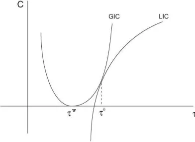
The lobby always makes a positive contribution. The intuition can be understood by looking at Figure 1, where the indifference curve of the government is described by a parabola (labelled GIC). Since the government is left with no surplus, the relevant indifference curve of the government is always the one corresponding to a domestic price equal to the welfare-maximizing price,τ =τW and zero contributions. The indifference
curve for the lobby (labelled LIC) is strictly increasing and convex inτ for q > 1ε1/ε
.
The equilibrium level of protection is determined by the tangency between the two indifference curves. Notice that at τ = τW the slope of the indifference curve of the
government is always zero as this is the tariff that maximizes aggregate welfare. So the lobby always has an incentive to contribute.
Figure 1: A Positive contribution in equilibrium
4
Entry and Exit
We now turn to the first stage of the game, where firms must decide to enter or not the industry. We assume the entry process is decentralized: that is, each firm makes its own decision, taking those of all other companies as given. To enter the industry in one of the countries, a firm bears the fixed costs of entry fE, measured in
labor units. An entrant then draws a productivity coefficientφ from a common ex-ante exogenous cumulative distributionJ(φ) in a subset of [0, ∞). Upon observing this draw, a firm may decide to exit and not produce. If it chooses to produce, however, it bears additional fixed overhead labor costsf, as in equation (9). If the firm chooses to export, it bears additional fixed costsfx, and we assume it will always serve its domestic market
is given by the one implicitly defined by equation (25), withτ◦
=τ◦
(n, n∗
, φx, φD), and
these expectations are fulfilled in equilibrium.
Profits from serving the local country and the foreign one are given respectively by equations (9) and by (10). The least productive firms expect negative operating profits and therefore exit the industry: this happens with all firms with productivity levels below a specific φD, which is the cutoff at which operating profits from domestic sales
equal zero. Firms with productivity levels betweenφD and φx have positive operating
profits from sales in the domestic market, but expect to lose money from exports, so they choose to serve only the domestic market. The cutoffφx is the productivity level
at which exporters just break even, so higher-productivity firms can export profitably. The cutoff coeficients for Home are
φε−1
D
1
εσ
1−ε qε−θ
(τ)
=f (30)
φx
τ
ε−1
1
εσ
1−ε q∗ε−θ
(τ∗
)
=fx (31)
Free entry ensures equality between the expected operating profits of a potential entrant and the entry costsfE. This condition can be expressed as
Z ∞
φD
πD(φ)dJ(φ) +
Z ∞
φx
πx(φ)dJ(φ) = fE (32)
There are equivalent conditions for Foreign. Equations (30), (31) and (32), for each country, provide implicit solutions for all the cutoff coefficients and the price indexes, given the expected tariff rate.
4.1 Number of Firms
To characterize the number of entrants in both countries, we can rewrite the price index as:
q=
n
Z ∞
φD
p(φ)1−εdJ(φ) +n∗
Z ∞
φ∗
x
p(φ)∗1−εdJ∗
(φ)
1/(1−ε)
with a similar equation for Foreign. The values of q and q∗
were determined in the previous subsection, so they can be written as
q1−ε =n
Z ∞
φD
p(φ)1−εdJ(φ) +n∗
Z ∞
φ∗
x
p(φ)∗1−εdJ∗
(φ) (34)
q∗1−ε =n
Z ∞
φx
p(φ)1−εdJ(φ) +n∗
Z ∞
φ∗
D
p(φ)∗1−εdJ∗
(φ) (35)
Aggregate spending in the economy must match aggregate revenue, so
Y =L=Lx0 +q
−θ
=⇒q= (L−Lx0)
−1/θ , q∗
= L∗
−L∗
x0
−1/θ
(36) Substituting back in equations(34) and (35), the number of firms can be implicitly determined.
To illustrate this, consider the case where both countries are equal. By solving equations (30), (31) and (32), using (36), an implicit solution for n and n∗ is obtained:
n=n∗
=
L−Lx0 (ε−1)fT
ε−1
· A(φD) +τ1−ε(φD, φx, n)A(φx)
−1
(37)
wherefT =A(φD)f+A(φx)fx+fE,A(φD) =
R
φDφε
−1dJφ) andA(φ
x) =
R
φxφε
−1dJ(φ).
5
Productivity distribution and the level of protection
where, holding the average constant, the size distribution of firms has a larger standard deviation, we can find a greater number of firms that are large enough to overcome the initial fixed cost of exporting. Larger firms gain a greater share of Home’s market and diminish the importance of local firms in lobbying for tariff protection.
Suppose productivities φ are distributed according to a Pareto distribution8 F(φ) with shape parameterη, in the support [φD,∞]. Supposeη >2. First, we must rewrite
the variables Γh and ΓI.
Γ◦
h =nβ
◦
Z ∞
φD
φε−1
dF(φ) (38)
Γ◦
I =n
∗ τ◦1−ε
β◦
Z ∞
φ∗
x
φε−1dF(φ) (39)
Now let’s parametrize F(φ) as Pareto distributions over the support given above. The probability density function for the firms isf(φ) =η(φφDη+1)η
If φ follows a pareto distribution with parameters η and φD, the variable S =φε−1
also follows a pareto distribution with shape ψ = ε−η1 and scale sD, where sD =φεD−1.
We restrict ψ >2 in order to keep the variance finite. It is possible to think of S as a variable representing sales, up to a constant.
We can rewrite the Γs as:
Γ◦
h =nβ
◦
Z ∞
sD
s ψsD
ψ
sψ+1ds=nβ
◦ ψ
ψ−1 ·sD (40)
Γ◦
I =n
∗
τ◦1−εβ◦ Z ∞
sx
s ψsD
ψ
sψ+1ds=n
∗
τ◦1−εβ◦ ψ ψ−1·sD
ψs
x1−ψ (41)
Now let us see the impact on the equilibrium tariff of changes in the shape param-eters. Consider the impact of a increase in the distribution of firms in both countries (fall inψ, caused by a fall inη or increase inε), maintaining the average firm constant, that is, a mean-preserving spread. The idea behind this is to capture precisely the effect of increased sectoral dispersion affecting the number of exporting firms in the foreign country and that sector protection in Home. Given the productivity cutoff necessary
8Axtell (2001) docummented that firm productivity closely follows this distribution. One can think
for firms to pay for the various fixed exporting costs and maintain an expected non-negative profit, an increased firm sectoral dispersion means more firms are able to cover these costs and export to Home.
Asψdecreases, the right tail of the distribution gets thicker and dispersion increases, so in order to maintain the average productivity constant sD has to fall. This lower
bound is related to the mean according to:
sD =µ
ψ−1
ψ (42)
whereµ is the average of the new Pareto variable S. Therefore we can rewrite ΓI as:
Γ◦
I =n
∗ τ◦1−ε
β◦ ψ ψ−1·sx
1−ψ·
µψ−1 ψ
ψ
(43)
Also, fix the export-cutoffsx: we want a condition on it such that the tariff responds
in a certan way to dispersion increases.
The are two ways through which a change in ψ affects ΓI: directly, as expressed
in the formula above, and indirectly, through the price index q, included in β◦
. In a continuous setting, we can rewriteq as:
q=
n
Z ∞
φD
p(φ)1−ε
dH(φ) +n∗
Z ∞
φ∗
x
p(φ)1−ε dF(φ)
1/(1−ε)
(44)
A change in ψ also affects Γh through q, in β◦. With this in mind, we can state the
following:
Proposition 3. An increase in foreign firm dispersion (fall inη) brings about a decrease
in the import tariff of the sector if the following condition is satisfied:
lnsx µ +ln
ψ ψ−1 >
1
ψ (45)
Proof: see appendix.
Observe that equation (45) is always satisfied if sx > µ. That’s it, the threshold
were satisfied, the ratio ΓI
Γh raises, implying that Foreign exporting firms gain market
in the Home. Thus, for equal countries, an increased productivity in the sector has a positive welfare effect on the equilibrium tariff. Increased dispersion augments the share of foreign firms as the larger ones have greater sales and some are much more profitable.
In contrast, in Bombardini (2005), increased firm dispersion changes the equilibrium tariff upward, due to the existence of a fixed cost for lobby and greater firm share and contributions. She finds a similar condition, since her problem is similar, also fitting the distribution to a Pareto. It is possible that Bombardini’s results overstate the true relationship between the tariff and the firm dispersion, since it neglects the effects of imports over the power of local firms, so it is an valid research topic to explore when these two different effects dominates. Our negative relationship between the equilibrium tariff and the sectorial dispersion is a testable proposition.
Now, let us see the impact of an increase inµ, keeping the dispersion constant and lettingSD vary
Proposition 4. An increase in the sector average productivity µ, in both countries,
brings about a decrease in the import tariff of the sector.
Proof: appendix.
Higher average productivity decreases production costs and so firms produce more. Although the effect considered here affects both countries, the average productivity of exporters increases more, causing a tariff decrease.
Finally, recall that the equilibrium conditions in section 4 gave us that sx sD =
τ◦ε−1fx
f
and defined≡ τ◦ε−1fx
f . Think ofdas a measure of the equilibrium relative cost premium
of exporters over non-exporters, everything else constant. Then, let us see the impact of a increase in the exporter’s cost premiumd, maintaining the lower bound sD fixed.
First, we write ΓI as:
Γ◦
I =n
∗ τ1−ε
β◦
sD
sx
ψ−1
=n∗ τ1−ε
β◦ d1−ψ
We can say that
Proposition 5. An increase in the sector relative cost of exporting d =τ◦ε−1f
x/f, in
both countries, brings about a increase in the import tariff of the sector.
Proof: appendix.
Increased costs naturally reduce the share of imports in Home and so the tariff increases. In a forthcoming paper, Das et al. (2007) show that different sectors have similar fixed costs of exporting. Then another interpretation for this results is that, at the equilibrium tariff, a sector which by some means attains a lower fixed cost, by improving its distributing network for example, is prone to have greater protection, presumely over the long-run.
6
Conclusion
We have developed in this paper a two-country model of international trade and lobbying in which firms competing in a monopolistic competition setting can, initially, choose to serve their domestic market or to export and, in a second stage, they organize a lobby to persuade the government to choose policies according to their own interests. These firms are heterogeneous in their productivities, so some do not enter the industry, others produce only for the domestic market and the most productive also export. Local firms that entered the industry lobby the government for protection in a manner `a la Grossman and Helpman. We obtain that, for equal countries, the equilibrium tariff falls with an increase in sector dispersion provided that the exporter’s cut-off firm is above the mean of the distribution. This is a testable proposition. Also it adds to the results from Bombardini (2005), who found that increased firm dispersion, in a setting with fixed costs for lobby formation, results in increased tariffs. Thus, in this paper, we find another effect of firm heterogeneity affecting the equilibrium tariff but in a opposite direction.
References
Axtell, Robert L., “Zipf Distribution of U.S. Firm Sizes,”Science, September 2001,
293, 1818–1820.
Bernard, Andrew B and J Bradford Jensen, “Exceptional Exporter Performance: Cause, Effect, or Both?,”Journal of International Economics, 1999, 47(1), 1–25.
Bernheim, Douglas and Michael Whinston, “Menu auctions, resource allocation and economic influence,”Quarterly Journal of Economics, february 1986, 101 (1).
Bombardini, Matilde, “Heterogeneity and Lobby Participation,”UBC working paper, 2005.
Chang, P, “Protection for sale under monopolistic competition,”Journal of Interna-tional Economics, 2005,66, 509–526.
Das, Roberts, and Tybout, “Market Entry Costs, Producer Heterogeneity, and Export Dynamics,”Econometrica, 2007. Forthcoming.
Findlay, Ronald and Stanislaw Wellisz, “Endogenous Tariffs, the Political Econ-omy of Trade Restrictions, and Welfare,” in J.N. Bhagwati, ed., Import competition and response, Chicago, IL: University of Chicago Press, 1982, pp. 223–234.
Flam, H. and E. Helpman, “Industrial policy under monopolistic competition,”
Journal of International Economics, 1987,22, 79–102.
Gros, D, “A note on the optimal tariff, retaliation and the welfare loss from tariff wars in a framework with intra-industry trade,”Journal of International Economics, 1987,
23, 357–367.
Grossman, G. and E. Helpman, “Foreign Investment with endogenous protection,” in R. Feenstra, G. Grossman, and D. Irwin, eds.,The political economy of trade policy: papers in honor of Jagdish Bhagwati, Cambridge, MA: MIT Press
”1996, pp. 199–224.
Helpman, E., M. J. Melitz, and S. R. Yeaple, “Export Versus FDI with Hetero-geneous Firms,”The American Economic Review, March 2004, 94 (1).
Hillman, Arye L., The political economy of protection, Vol. 32 of Fundamentals of Pure and Applied Economics, Chur, Switzerland: Harwood Academic Publishers, 1989.
Melitz, Marc J, “The impact of trade on intra-industry reallocations and aggregate industry productivity,”Econometrica, 2003, 71(6), 1695–1725.
Mitra, Devashish, “Endogenous Lobby Formation and Endogenous Protection: A Long-Run Model of Trade Policy Determination,”American Economic Review, 1999,
89 (5), 1116–34.
Montagna, C, “Monopolistic competition with firm specific costs,”Oxford Economic Papers, 1995,47 (2), 318–328.
Rodrik, Dani, “Political Economy of Trade Policy,” in Gene M. Grossman and Kenneth Rogoff, eds., Handbook of international economics, Vol. 3 1995.
Yeaple, S, “A Simple Model of Firm Heterogeneity, International Trade, and Wages,”
Appendix A
Value of contributions in equilibirum. First, let’s declare a result to be used later.
Lemma. Takeτ◦
andτ−i given respectively by (25)and (28). Thenq(τ◦)
> q(τ−i).
Proof. Given that Ci(τ, B◦) = Wi(τ)−Bi◦, we have that Ci(τ−i, B◦)−Ci(τ◦, B◦) = Wi(τ−i)−
Wi(τ◦) = Πi(τ−i)−Πi(τ◦). ButCi(τ−i, B◦) = 0 andCi(τ◦, B◦)>0, implying Πi(τ◦)>Πi(τ−i). But
this happens if and only ifqε−θ(τ◦)
> qε−θ(τ−i).
LetR(τ−i, τ◦
) =(τ−τ−i−i1)
P
k∈Ipk,f(τ−i)xk,f(τ−i)−(τ
◦−1)
τ◦
P
k∈Ipk,f(τ◦)xk,f(τ◦) andm(τ−i, τ◦) =
1
θ−1 q
1−θ(τ−i)−q1−θ(τ◦)
. From the definition ofW(·), we have that
W(τ−i)−W(τ◦
) = X
k∈N
πk(τ−i)−πk(τ◦)+R(τ−i, τ◦) +m(τ−i, τ◦)
= X
k∈N
1
ε
φk
σ
ε−1
qε−θ(τ−i)−qε−θ(τ◦
)
+R(τ−i, τ◦
) +m(τ−i, τ◦
)
Then
C◦
i =a W(τ
−i
−W(τ◦
))
= qε−θ(τ−i)−qε−θ(τ◦
) 1
σε−1ε
"
aX
k∈N
φε−1
k #
+a R(τ−i, τ◦
) +m(τ−i, τ◦
) (A-1)
The contribution is positive considering the lemma proved just before. Basically, the consumer surplus is high enough to compensate for the fall in profits from the policyτ−i.
Proof of Proposition 3. From the first-order condition, define
Ω =−ε(a+α)(τ−1)(ε−(ε−θ)ΓI) +τ(a+ 1)(ε−θ)Γh
So, by the implicit function theorem, we have
∂τ ∂ψ =−
∂Ω
∂ψ ∂Ω
∂τ
The denumerator is the second-order condition, so it is negative by assumption. We need the sign of the numerator.
∂Ω
∂ψ =ε(a+α)(τ−1)(ε−θ) ∂ΓI
∂ψ +τ(a+ 1)(ε−θ) ∂Γh
∂ψ
We have that Γh and Γf are given by (40) and (41), but some notation is necessary: letG(ψD) = R∞
sDs ψ
sDψ
sψ+1ds=µ, andG(ψ) = R∞
sx s ψ
sDψ
sψ+1ds= ψ ψ−1·sx
1−ψ·µψ−1
ψ ψ
This way, let’s calculate the derivatives from the formula above.
∂Γh
∂ψ =n G(ψ)D ∂β◦
∂ψ +G(ψ)Dβ
◦∂n
∂ψ
=G(ψ)Dβ◦
∂n
∂ψ(1−nβ
◦
G(ψ)D)−nτ1−εG(ψ)Dβ◦2
∂n∗
∂ψG(ψ) +n
∗∂G(ψ)
∂ψ
=G(ψ)Dβ◦
∂n
∂ψ(1−Γh)−Γhτ
1−εβ◦
∂n∗
∂ψG(ψ) +n
∗∂G(ψ)
∂ψ
and
∂ΓI
∂ψ = ∂n∗
∂ψτ
1−εβ◦
G(ψ) +n∗
τ1−ε
∂β◦
∂ψ G(ψ) +β
◦∂G(ψ)
∂ψ
=β◦
τ1−ε
G(ψ)∂n
∗
∂ψ +n
∗∂G(ψ)
∂ψ
1−τ1−εβ◦
n∗
G(ψ) −
G(ψ)Dτ1−εβ◦2G(ψ)
∂n ∂ψ
=β◦
τ1−ε
G(ψ)∂n
∗
∂ψ +n
∗∂G(ψ)
∂ψ
(1−ΓI)−G(ψ)Dβ◦ΓI
∂n ∂ψ
where ΓI and Γh<1.
Since Γh= 1−ΓI, ∂∂ψΓI =−∂∂ψΓh. Substituting back in (6):
∂Ω
∂ψ = ∂ΓI
∂ψ {ε(a+α)(τ−1)(ε−θ)−τ(a+ 1)(ε−θ)}
=
β◦
τ1−ε
G(ψ)∂n
∗
∂ψ +n
∗∂G(ψ)
∂ψ
(1−ΓI)−G(ψ)Dβ◦ΓI
∂n ∂ψ
×
ε(a+α)(τ−1)−τ(a+ 1)
=β◦
τ1−εσ1−ε
G(ψ)∂n
∗
∂ψ +n
∗∂G(ψ)
∂ψ
nG(ψ)D−n∗G(ψ)DG(ψ)
∂n ∂ψ
×
ε(a+α)(τ−1)−τ(a+ 1)
But the term in brackets is negative, since from the first-order condition
τ◦
−1
τ◦ =
a+ 1
ε(a+α)·
(ε−θ)Γ◦
h
(ε−(ε−θ)Γ◦
I)
< a+ 1 ε(a+α) due to
(ε−θ)Γ◦
h
(ε−(ε−θ)Γ◦
I)
= (ε−θ)Γ
◦
h
(θ+ (ε−θ)Γ◦
h)
<1 So,
∂Ω
∂ψ >0 and ∂τ ∂ψ >0
m
G(ψ)∂n
∗
∂ψ +n
∗∂G(ψ)
∂ψ
nG(ψ)D−n∗G(ψ)DG(ψ)
∂n ∂ψ
<0
Countrie are equal, so the derivatives and number of firms are equal. Therefore this inequality collapses to
∂G(ψ)
∂ψ <0 ⇔ ln φI
µ +ln ψ ψ−1 >
1
ψ (A-2)
Proof of Proposition 4. Continuing from the last proof, we have that:
∂Ω
∂µ = − ∂Γh
As before the second term in the right is negative. But
∂Γh
∂µ =nβ
◦
+nG(ψ)D
∂β◦
∂µ
= +nβ◦
−nβ◦
Γh−n2β◦2G(ψ)Dτ1−ε
sD
sx ψ−1
=nβ◦
−Γ
2
h
µ −
ΓhΓIψ
µ
=⇒ ∂Ω
∂µ <0 and ∂τ ∂µ <0
m
nβ◦
−Γ
2
h
µ −
ΓhΓIψ
µ <0
m
ψ >1, which is valid by assumption.
Proof of Proposition 5.
∂Ω
∂d = ∂ΓI
∂d {ε(a+α)(τ−1)(ε−θ)−τ(a+ 1)(ε−θ)}
As before, the second term in the right is negative. However,
∂ΓI
∂d =n
∗
β2◦
τ1−εµ(1−ψ)d−ψ(1−Γ I)<0