Artificial satellites dynamics: Resonant effects

(1)

ARTIFICIAL SATELLITES DYNAMICS: RESONANT EFFECTS

Jarbas Cordeiro Sampaio

UNESP- Univ Estadual Paulista, CEP. 12516-410 Guaratinguetá-SP, Brazil, jarbascordeiro@gmail.com

Rodolpho Vilhena de Moraes

UNIFESP- Univ Federal de São Paulo, CEP. 12231-280 São José dos Campos, SP, Brazil, rodolpho.vilhena@gmail.com

Sandro da Silva Fernandes

ITA- Inst Tecnológico de Aeronáutica, CEP. 12228-900 São José dos Campos, SP, Brazil, sandro@ita.br

Abstract: In this work, the resonance problem in the artificial satellites motion is studied. The development of the

geopotential includes the zonal harmonicsJ20andJ40and the tesseral harmonicsJ22andJ42. Through succes-sive Mathieu transformations, the order of dynamical system is reduced and the final system is solved by numerical integration. In the simplified dynamical model, two critical angles are studied,φ2201andφ4211. Numerical results show the time behavior of the semi-major axis andφ2angle.

Keywords: Artificial Satellites. Resonance. Orbits.

1 Introduction

Synchronous satellites in circular or elliptical orbits have been extensively used for navigation, communication and military missions. This fact justifies the great attention that has been given in literature to the study of resonant orbits characterizing the dynamics of these satelli-tes since the 60’s (Morando, 1963; Blitzer, 1963; Garfinkel, 1965a; Garfinkel, 1965b; Garfinkel, 1966; Gedeon and Dial, 1967; Gedeon et al., 1967; Gedeon, 1969; Lane, 1988; Jupp, 1969; Ely and Howell, 1996). For example, Molniya series satellites used by the old Soviet Union for communication form a constellation of approximately 110 satellites, launched since 1965, which have highly eccentric orbits with periods of 12 hours. Another example of missions that use eccentric orbits, inclined and synchronous, include satellites to investigate the solar magnetosphere, launched in the 90’s (Neto, 2006).

The orbits of synchronous satellites are very complex. The tesseral harmonics of the geopotential produce multiple resonances which interact resulting significantly nonlinear motions, when compared to non-resonant orbits. It has been found that the orbital elements show relatively large oscillation amplitudes differing from neighboring trajectories, they are in fact chaotic (Ely and Howell, 1996). It should also be noted that the characteristics of several missions involving such orbits require that they are kept to a minimum fuel consumption. Geographic requirements determined by the missions and spatial maneuvers of minimum cost demand precise control of the trajectories that are subjected to significant nonlinearities during the satellite lifetime.

In this paper, the 2:1 resonance is considered; in other words, the satellite completes two revolutions while the Earth carries one.

2 The Resonance Problem

In this section, a simplified Hamiltonian describing the resonant problem is derived through sucessive Mathieu transformations.

Consider Eq. (1) to the Earth gravitational potential written in classical orbital elements (Osorio, 1973; Kaula, 1966)

V = µ 2a+

∞

X

l=2 l

X

m=0 l

X

p=0

−∞

X

q=+∞

µ a

a_e

a

l

JlmFlmp(I)Glpq(e)cos(φlmpq(M, ω,Ω,Θ)), (1)

(2)

ais the semi-major axis,e is the eccentricity,I is the inclination of the orbit plane with the equator,Ωis the longitude of the ascending node,ω is the argument of pericentre andM is the mean anomaly, respectively; ae is the Earth mean equatorial radius,ae=6378.140 km,Jlm is the spherical harmonic coefficient of degreeland orderm, Flmp(I) andGlpq(e) are Kaula’s inclination and eccentricity functions, respectively. The argument φlmpq(M, ω,Ω,Θ)is defined by

φlmpq(M, ω,Ω,Θ) =qM+ (l₋2p)ω+m(Ω₋Θ₋λlm) + (l₋m) π

2 ,

whereΘis the Greenwich sidereal time andλlmis the corresponding reference longitude along the equator.

In order to describe the problem in Hamiltonian form, Delaunay canonical variables are introduced

L=√µa G=p

µa(1₋e2₎ _H₌p

µa(1₋e2₎_cos₍_I₎

l=M g=ω h= Ω. (2)

Using the canonical variables, one gets the HamiltonianFˆ,

ˆ

F = µ

2

2L2 +

∞

X

l=2 l

X

m=0

Rlm , (3)

with the disturbing potentialRlmgiven by

Rlm = l

X

p=0 +∞

X

q=−∞

Blmpq(L, G, H)cos(φlmpq(l, g, h,Θ)). (4)

The argumentφlmpqis defined by

φlmpq(l, g, h,Θ) =ql+ (l₋2p)g+m(h₋Θ₋λlm) + (l₋m) π

2 , (5)

and the coefficientBlmpq(L, G, H)by

Blmpq = ∞

X

l=2 l

X

m=0 l

X

p=0

−∞

X

q=+∞

µ2 L2

µa_e

L2

l

JlmFlmp(L, G, H)H

−(l+1),(l−2p)

q (L, G). (6)

The HamiltonianFˆ depends explicitly on the time through the Greenwich sidereal timeΘ, whereΘ = Ωet(Ωeis the Earth’s angular velocity andtis the time). A new variableθ, conjugated toΘ, is introduced in order to extend the phase space. In the extended phase space, the extended HamiltonianHˆ is given by

ˆ

(3)

For resonant orbits, it is convenient to use a new set of canonical variables. Consider the canonical transformation of variables defined by the following relations

X =L Y =G₋L Z=H₋G Θ = Θ

x=l+g+h y=g+h z=h θ=θ , (8)

whereX, Y, Z,Θ, x, y, z, θare the modified Delaunay variables.

The new HamiltonianHˆ′_{, resulting from the canonical transformation defined by Eq. (8), is given by}

ˆ

H′₌ µ

2

2X2+ωeθ+

∞

X

l=2 l

X

m=0 R′

lm, (9)

where the disturbing potentialRlm′ is given by

R′lm = l

X

p=0 +∞

X

q=−∞

Blmpq′ (X, Y, Z)cos(φlmpq(x, y, z,Θ)). (10)

Consider the resonance to be studied in this work; that is, the commensurability between the Earth rotation angular velocityΩeand the mean motionn. This commensurability can be expressed as

qn₋mωe∼= 0 (11)

consideringqandmas integers. The commensurability of the resonance studied,q/m, is defined byα. When this commensurability ocurrs, small divisors, associated to the tesseral harmonics, arise in the integration of the equations of motion (Lane, 1988). These terms are called resonants.

The short and long period terms can be eliminated from the HamiltonianHˆ′_{by applying an averaging method. A} reduced HamiltonianHˆris obtained from the HamiltonianHˆ′ when only secular and resonant terms are consid-ered. Several authors, Kaula (1966), Lima Jr (1998), Formiga and Vilhena de Moraes (2009), Vilhena de Moraes et al. (1995), Ely and Howell (1996) also use this simplified Hamiltonian to study the resonance. The reduced HamiltonianHˆris given by

ˆ

Hr= µ2

2X2+ωeθ+

∞

X

j=1

B₂′_j,₀_,j,₀(X, Y, Z)+

+ ∞

X

l=2 l

X

m=2 l

X

p=0

B′lmp(αm)(X, Y, Z)cos(φlmp(αm)(x, y, z,Θ)). (12)

The canonical system of differential equations governed byHˆrhas the first integral

1₋1

α

(4)

whereC1is an integration constant.

Using this first integral, a Mathieu transformation

(X, Y, Z,Θ, x, y, z, θ)_→(X1, Y1, Z1,Θ1, x1, y1, z1, θ1)

can be defined.

This transformation is given by the following equations

X1=X Y1=Y Z1=

1− 1 α

X+Y +Z Θ1= Θ

x1=x₋

1₋ 1

α

z y1=y₋z z1=z θ1=θ. (14)

The subscript 1 denotes the new set of canonical variables. Note thatZ1=C1and thez1is an ignorable variable. So, the order of the dynamical system is reduced in one degree of freedom.

Substituting the new set of canonical variables,X1, Y1, Z1,Θ1, x1, y1, z1, θ1, in the reduced Hamiltonian given by Eq. (12), one gets the resonant Hamiltonian. The word "resonant" is used to denote the HamiltonianH1ˆ ,rswhich is valid for any resonance. The periodic terms in this Hamiltonian are resonant terms. The HamiltonianH1ˆ ,rsis given by

ˆ

H1,rs= µ2

2X2 1

+ωeθ1+ ∞

X

j=1

B1,2j,0,j,0(X1, Y1, Z1)+

+ ∞

X

l=2 l

X

m=2 l

X

p=0

B1,lmp,(αm)(X1, Y1, Z1)cos(φ1,lmp(αm)(x1, y1, z1,Θ1)). (15)

The HamiltonianH1ˆ ,rs has all resonant frequencies, relative to the commensurabilityα, where theφ1,lmp(αm)

argument is given by

φ1,lmp(αm)=m(αx1−Θ1) + (l−2p−αm)y1−φ1,lmp(αm)0, (16)

with

φ1,lmp(αm)0=mλlm₋(l₋m) π

2. (17)

The secular and resonant terms are given, respectively, byB1,2j,0,j,0(X1, Y1, Z1)and B1,lmp(αm)(X1, Y1, Z1).

Each one of the frequencies contained in dx1 dt,

dy1 dt,

dΘ1

dt is related, through the coefficientsl, m, to a tesseral harmonicJlm. By varying the coefficientsl,m,pand keepingq/mfixed, one finds, all frequencies

(5)

Now, consider a single frequency among the several resonant frequencies that can be obtained from the expression

φ1,lmp(αm)

dt =m

αdx1 dt −

dΘ1 dt

+ (l₋2p₋mα)dy1

dt . (18)

The frequencyφ˙1,lmp(αm)for the fixed coefficientsmand(l−2p−mα)will be the unique resonant frequency

considered in the resonant HamiltonianH1ˆ ,rs. This frequency will be called "critical frequency".

A critical frequency can be, for example, the one that results in a smaller numerical value forφ1˙ ,lmp(αm), implying

a effect strengthening of the resonance considered. The frequencies of the argumentsΩandωcan become more pronounced the presence of small divisors that arise in the integration of the motion equations, this depend also on the eccentricity and inclination of the orbit plane. The importance of the node and the pericentre frequencies is smaller when compared to the mean anomaly and Greenwich sidereal time, however, they also have their contri-bution in the resonance effect. As mentioned in preceding paragraphs, the coefficientsl,m,pcan vary, producing different frequencies within the resonant cosines for the same resonance. These frequencies are slightly different, with small variations around the commensurability given byαx1˙ -Θ˙1.

In the keplerian elements, the coefficient of frequencyω˙ assumes the values 2, 0, -2, and the coefficient of frequency ˙

y1assumes the values 1, -1, -3.

According to Eq. (16), the argument in the resonant Hamiltonian is given by

φ1,lmp(αm)(x1, y1,Θ1). To determine a critical frequency, one needs to fix all the coefficients of the variablex1, y1,Θ1; in other words, one fixesα,mand (l-2p-mα).

The coefficientαis fixed, because the type of resonance is defined; in this paper 2:1. Once the resonant angle has been chosen, the coefficientsmand (l-2p-mα) must be fixed too.

By fixing the expressionl₋2pinstead of the coefficientsl andpseparately, one has the possibility to varyl

andp, considering thatl₋2pis a certain fixed value k. Once this critical frequency has been chosen among the possible resonant frequencies, the other periodic terms of the HamiltonianH1ˆ,rsare taken as short period terms, with frequencies different from the critical frequency.

Defining a single critical frequency, or, assuming the isolated study of each frequency, a new Hamiltonian is obtained. This new Hamiltonian is given by

ˆ

H1,c= µ2

2X2 1

+ωeθ1+ ∞

X

j=1

B1,2j,0,j,0(X1, Y1, C1)+

+ ∞ X l=2 l X p=0

B1,lmp,(αm)(X1, Y1, C1)cos(φ1,lmp(αm)(x1, y1,Θ1)). (19)

The coefficientsk=l₋2pandmare fixed. This Hamiltonian contains secular and critical terms only. Sincekis a fixed value,H1ˆ ,ccan be put in the simplified form

ˆ

H1,c= µ2

2X₁2+ωeθ1+

∞

X

j=1

B1,2j,0,j,0(X1, Y1, C1)+

+ ∞

X

p=S

B1,lmp,(αm)(X1, Y1, C1)cos(φ1,lmp(αm)(x1, y1,Θ1)), (20)

where µ2 2X2

1

+

ω

_e

θ

₁is the central part of the Hamiltonian, ∞

P

j=1

B1,2j,0,j,0(X1, Y1, C1)contains only secular terms

(6)

∞

X

p=s

B1,(2p+k)mp(αm)(X1, Y1, C1)cosφ1,(2p+k)mp(αm)(x1, y1,Θ1)

represents the resonant terms that have the same critical frequency.

The canonical system of differential equations governed by the HamiltonianH1ˆ ,chas the first integral

(k₋mα)X1₋mαY1=C2, (21)

whereC2is an integration constant.

Using this integral, a new Mathieu transformation can be defined. This canonical transformation is given by the following equations

X2=X1 Y2= (k₋mα)X1₋mαY1 Θ2= Θ1

x2=x1+

_k

−mα

mα

y1 y2=₋ 1

mαy1 θ2=θ1. (22)

The subscript 2 denotes the new set of canonical variables.

The Hamiltonian function is invariant with respect to this new Mathieu transformation. Thus, from Eq. (20) and (22), one gets the final HamiltonianH2ˆ ,f

ˆ

H2,f = µ2

2X22

+ωeθ2+ ∞

X

j=1

B2,2j,0,j,0(X2, C1, C2)+

+ ∞

X

p=S

B2,(2p+k)mp(αm)(X2, C1, C2)cos(φ2,(2p+k)mp(αm)(x2,Θ2)), (23)

where ∞

P

j=1

B2,2j,0,j,0(X2, C1, C2)represents the secular terms and

∞

X

p=s

B2,(2p+k)mp(αm)(X2, C1, C2)cosφ1,(2p+k)mp(αm)(x2,Θ2)

represents the resonant terms with the same critical frequencies. Note thatY2=C2andy2is an ignorable variable.

The new angleφ2,(2p+k)mp(αm)(x2,Θ2)is given by

φ2,(2p+k)mp(αm)(x2,Θ2) =φ2−φ2,(2p+k)mp(αm),0, (24)

(7)

φ2,(2p+k)mp(α),0=mλ(2p+k)m−(2p+k−m) π

2 =φ1,lmp(αm)0. (25)

Recall thatkandmare two fixed coefficients determined by choosing a critical resonant frequency, among the sev-eral possible resonant frequencies. The HamiltonianH2ˆ ,f has all tesseral related to the chosen critical frequency.

For small eccentricities, the Hansen’s coefficients can be expressed in Newcomb’s polynomials and Kaula’s eccen-tricity function (Kaula, 1966):

H−(2p+k+1),k

αm (e) =G(2p+k)p(αm)(e). (26)

Accordingly, the HamiltonianHˆ′

2,f can be rewritten as

ˆ

H′

2,f = µ2

2X2 2

+ωeθ2+ ∞

X

j=1

B2,2j,0,j,0(X2, C1, C2)+

+ ∞

X

p=S

B2,(2p+k)mp(αm)(X2, C1, C2)cos(φ2,(2p+k)mp(αm)(x2,Θ2)), (27)

with

B2,(2p+k)mp(αm)(X2, C1, C2) =

µ2p+k+2 X4p+2k+2a

2p+k

e J(2p+k)m×

×F(2p+k)mp(X2, C1, C2)G(2p+k)p(αm)(X2, C2), (28)

where the functionGlpq(e)is the Kaula’s eccentricity function. Prime denotes the simplified Hamiltonian for small eccentricities.

The dynamical system generated by HamiltonianHˆ′

2,fis

dX2

dt =−mα

∞

X

p=S

B2,(2p+k)mp(αm)(X2, C1, C2)sen(φ2,(2p+k)mp(αm)) (29)

dφ2 dt =mα

µ2 X3

2 −

mωe₋mα ∞

X

j=1

∂B2,2j,0,j,0(X2, C1, C2)

∂X2 −

−mα

∞

X

p=S

∂B2,(2p+k)mp(αm)(X2, C1, C2)

∂X2 cos(φ2,(2p+k)mp(αm)(x2,Θ2)) (30)

The Eq. (29) and (30) represent the motion equations in a resonance of commensurabilityα.

3 Results

Figures (1) to (8) show the time behavior of the semi-major axis andφ2angle, according to the numerical integra-tion of the mointegra-tion equaintegra-tions, (29) and (30). The initial condiintegra-tions, in the Figs. (1) to (8), for inclinaintegra-tions are100

and550_{, and eccentricities, 0.001 and 0.01. The initial values of semi-major axis are around the critical semi-major}

(8)

-1000 -500 0 500 1000 1500 2000 2500

0 1000 2000 3000 4000 5000 6000 7000 8000 φ2

(degrees)

t (days)

circulation libration

Figure 1.φ2versus t, considering the tesseral harmonicJ22. The initial conditions for inclination and eccentricity are

I = 10o

and e=0.001, respectively

26546 26548 26550 26552 26554 26556 26558 26560 26562 26564

0 1000 2000 3000 4000 5000 6000 7000 8000

a (Km)

t (days)

Figure 2.aversus t, considering the tesseral harmonicJ22. The initial conditions for inclination and eccentricity are

I = 10o

(9)

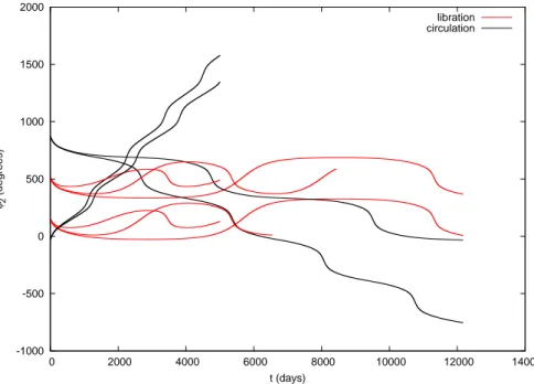
-1000 -500 0 500 1000 1500 2000

0 2000 4000 6000 8000 10000 12000 14000

φ2

(degrees)

t (days)

libration circulation

I = 55o

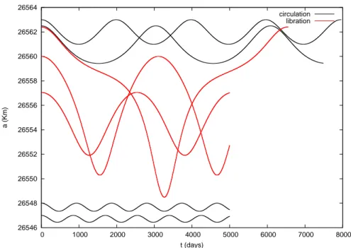
26554 26556 26558 26560 26562 26564 26566 26568

0 2000 4000 6000 8000 10000 12000 14000

a (Km)

t (days)

I = 55o

(10)

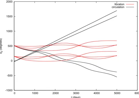
-1500 -1000 -500 0 500 1000 1500 2000 2500

0 1000 2000 3000 4000 5000 6000 7000 8000 φ2

(degrees)

t (days)

I= 10o

26540 26545 26550 26555 26560 26565 26570

0 1000 2000 3000 4000 5000 6000 7000 8000

a (Km)

t (days)

I= 10o

(11)

-1000 -500 0 500 1000 1500 2000

0 1000 2000 3000 4000 5000 6000

φ2

(degrees)

t (days)

I= 55o

26552 26554 26556 26558 26560 26562 26564 26566 26568 26570

0 1000 2000 3000 4000 5000 6000

a (Km)

t (days)

I= 55o

(12)

Figures (1) to (8) show that vibration amplitudes increasing when the inclination varies from 10oto 55oand when the eccentricity varies from 0.001 to 0.01. Figures (9) and (10) show the time behavior of the semi-major axis andφ2angle, considering the critical angleφ2201associated to tesseral harmonicJ22and the critical angleφ4211

associated to tesseral harmonicJ42. The Table 1 show the resonant coefficients.

Table 1. Resonant coefficients

Degree (l) Order (m) p q

2 2 0 1

4 2 1 1

26540 26545 26550 26555 26560 26565 26570

0 2000 4000 6000 8000 10000

a (Km)

t (days)

J₂₂ J₂₂ and J₄₂

Figure 9.aversus t, considering the tesseral harmonicsJ22andJ42. The initial conditions for inclination and eccentricity areI = 10o

-2000 -1500 -1000 -500 0 500 1000 1500 2000 2500

0 2000 4000 6000 8000 10000

φ2

(degrees)

t (days)

J₂₂ J22 and J42

Figure 10.φ2versus t, considering the tesseral harmonicJ22andJ42. The initial conditions for inclination and eccentricity areI = 10o

Figures (9) and (10) show the difference in the time behavior of the semi-major axis andφ2angle, with the addition of the tesseral harmonicJ42. The tesseral harmonicJ42is∼=O(10−6₎_{and it changes the value of the critical}

(13)

µ2 X3

2 −

2ωe₋ ∞

X

j=1

∂B2,2j,0,j,0(X2, C1, C2)

∂X2 = 0. (31)

Table 2. Critical semi-major axis

Eccentricity Inclination (o) Critical angle Semi-major axis (km)

0.001 10 φ2201 26557.05255

0.001 55 φ2201 26562.59742

0.01 10 φ2201 26557.05208

0.01 55 φ2201 26562.59758

0.001 10 φ2201+φ4211 26557.05194

0.001 55 φ2201+φ4211 26562.59767

0.01 10 φ2201+φ4211 26557.05148

0.01 55 φ2201+φ4211 26562.59783

4 Conclusions

In this work, the dynamical behavior of two critical angles associated to the 2:1 resonance problem in the artifi-cial satellites motion have been investigated. Through successive canonical transformations, a simplified model describing the problem is derived. In the regular motion region, one can study the dynamical system considering each critical angle separately.

The results show the time behavior of the semi-major axis andφ2angle, considering two inclinations, 100_and

550_{, and different eccentricities, 0.001 and 0.01. Two different regions are observed in the numerical integration,}

libration and circulation regions.

Two critical angles are studied,φ2201 associated toJ22andφ4211associated to J42. The values of the critical semi-major axis show a difference of centimeters in the libration region, when the tesseral harmonicJ42is added.

Inside the region where the resonances are found, the motion can be chaotic, because it shows sensibility to initial conditions.

5 Acknowledgements

This work was accomplished with support of the FAPESP under the contract No_{2009/00735-5 and 2006/04997-6,} SP-Brazil, and CNPQ (contracts 300952/2008-2 and 302949/2009-7).

6 References

Morando, M. B. Orbites de Resonance des Satellites de 24h. Bull. Astron. 24, pp. 47, 1963.

Blitzer, L. Synchronous and Resonant Satellite Orbits Associated with Equatorial Ellipticity. ARS Journal 32, pp. 1016-1019, 1963.

Garfinkel, B. The Disturbing Function for an Artificial Satellite. Astron. Journal, Vol. 70, pp. 688-704, 1965a. Garfinkel, B. Tesseral Harmonic Perturbations of an Artificial Satellite. Astron. Journal, Vol. 70, pp. 784-786,

1965b.

Garfinkel, B. Formal Solution in the Problem of Small Divisors. Astron. Journal, Vol. 71, pp. 657-669, 1966. Gedeon, G. S; Dial, O. L. Along-track Oscillations of a Satellite due to Tesseral Harmonics. AIAA Journal, Vol. 5,

pp. 593-595, 1967.

Gedeon, G. S; Douglas, B. C; Palmiter, M. T. Resonance Effects on Eccentric Satellite Orbits. Journal of the Astronautical Sciences, Vol. XIV, pp. 147-157, 1967.

Gedeon, G. S. Tesseral Resonance Effects on Satellite Orbits. Celestial Mechanics 1, pp. 167-189, 1969.

(14)

Jupp, A. A Solution of the Ideal Resonance Problem for the Case of Libration. Astron. Journal, Vol. 74, pp. 35-43, 1969.

Ely, T. A; Howell, K. C. Long-term Evolution of Artificial Satellite Orbits due to Resonant Tesseral Harmonics. Journal of the Astronautical Sciences, Vol. 44, pp. 167-190, 1996.

Neto, A. G. S.. Estudo de Órbitas Ressonantes no Movimento de Satélites Artificiais. Tese de Mestrado, ITA, 2006. Osorio, J. P.. Perturbações de Órbitas de Satélites no Estudo do Campo Gravitacional Terrestre. Porto, Imprensa

Portuguesa, 1973.

Kaula, W. M. Theory of Satellite Geodesy:Applications of Satellites to Geodesy. Blaisdel Publ. Co., Waltham, Mass, 1966.

Lima Jr, P. H. C. N. Sistemas Ressonantes a Altas Excentricidades no Movimento de Satélites Artificiais. Tese de Doutorado, Instituto Tecnológico de Aeronáutica, 1998.

Grosso, P. R. Movimento Orbital de um Satélite Artificial em Ressonância 2:1. Tese de Mestrado, Instituto Tec-nológico de Aeronáutica, 1989.

Formiga, J. K. S.; Vilhena de Moraes, R. Dynamical systems: an integrable kernel for resonance effects. Journal of Computational Interdisciplinary Sciences 1(2): pp. 89-94, 2009.