Free vibration analysis of an embarked rotating composite shaft
using the hp- version of the FEM
Abstract
This paper presents the study of the vibratory behavior of rotating composite shafts. The composite shaft contains isotropic rigid disks and is supported by bearings that are modeled as springs and viscous dampers. An hp- version of the Finite Element Method (FEM) is used to model the structure. A hierarchical finite element of beam type with six degrees of freedom per node is developed. The assembly is made by the standard version of the finite element method for several elements. A theoretical study allows the estab-lishment of the kinetic energy and the strain energy of the system (shaft, disk and bearings) necessary to the result of the equations of motion. In this study the transverse shear deformation, rotary inertia and gyroscopic effects, as well as the coupling effect due to the lamination of composite lay-ers have been incorporated. A program is elaborate for the calculation of the eigen-frequencies and critical speeds of the system. The results obtained compared with those available in the literature show the speed of convergence, the exacti-tude and the effectiveness of the method used. Several exam-ples are treated, and a discussion is established to determine the influence of the various parameters and boundary condi-tions.
Keywords
rotating shaft, disk, composite materials, gyroscopic effect,
hp- version, hierarchical finite element method, FEM.
Abdelkrim Boukhalfa∗
and Abdelhamid Hadjoui
Department of Mechanical Engineering, Fac-ulty of Sciences Engineering, Abou Bakr Belkaid University, Tlemcen, 13000 – Algeria
Received 19 Oct 2009; In revised form 25 Feb 2010 ∗Author email: [email protected]
1 INTRODUCTION
damp-NOMENCLATURE
U(x, y, z) Displacement inx direction. V(x, y, z) Displacement iny direction. W(x, y, z) Displacement inz direction.
βx Rotation angles of the cross-section about they axis.
βy Rotation angles of the cross-section, about thez axis.
φ Angular displacement of the cross-section due to the torsion deformation of the shaft.
E Young modulus.
G Shear modulus.
(1, 2, 3) Principal axes of a layer of laminate
(x, y, z) Cartesian coordinates.
(x, r,θ) Cylindrical coordinates.
Gc Centre of the cross-section.
(O,x, y, z) Inertial reference frame.
(Gc,x1,y1,z1) Local reference frame is located in the centre of the cross-section.
C′
ij Elastic constants.
ks Shear correction factor.
ν Poisson coefficient.
ρ Masse density.
L Length of the shaft.
D Mean radius of the shaft.
e Wall thickness of the shaft.
Rn Thenth layer inner radius of the composite shaft.
Rn+1 Thenth layer outer radius of the composite shaft.
k Number of the layer of the composite shaft.
η Lamination (ply) angle.
θ Circumferential coordinate.
ξ Local and non-dimensional co-ordinates.
ω Frequency, eigen-value.
Ω Rotating speed.
[N] Matrix of the shape functions.
f (ξ) Shape functions.
p Number of the shape functions or number of hierarchical terms.
t Time.
Ec Kinetic energy.
Ed Strain energy.
{qi} Generalized coordinates, with (i = U, V, W,βx,βy,φ)
[M] Masse matrix.
[K] Stiffness matrix.
[G] Gyroscopic matrix.
[Cp] Damping matrix.
Kyy0, Kyz0, Kzy0, Kzz0 Bearing stiffness coefficients in x = 0.
KyyL, KyzL, KzyL, KzzL Bearing stiffness coefficients in x =L.
Cyy0, Cyz0, Czy0, Czz0 Bearing damping coefficients in x = 0.
ing etc. The solutions proposed are just adequate, but require substantial refinements, which might explain some of the differing experiences of various authors.
Zinberg and Symmonds [27] described a boron/epoxy composite tail rotor driveshaft for a helicopter. The critical speeds were determined using equivalent modulus beam theory (EMBT), assuming the shaft to be a thin walled circular tube simply supported at the ends. Shear deformation was not taken into account. The shaft critical speed was determined by extrapolation of the unbalance response curve which was obtained in the sub-critical region.
Dos Reis et al. [12] published analytical investigations on thin-walled layered composite cylindrical tubes. In part III of the series of publications, the beam element was extended to formulate the problem of a rotor supported on general eight coefficient bearings. Results were obtained for shaft configuration of Zinberg and Symmonds. The authors have shown that bending-stretching coupling and shear-normal coupling effects change with stacking sequence, and alter the frequency values. Gupta and Singh [13] studied the effect of shear-normal coupling on rotor natural frequencies and modal damping. Kim and Bert [15] have formulated the problem of determination of critical speeds of a composite shaft including the effects of bending-twisting coupling. The shaft was modeled as a Bresse-Timoshenko beam. The shaft gyroscopics have also been included. The results compare well with Zinberg’s rotor [27]. In another study, Bert and Kim [4] have analysed the dynamic instability of a composite drive shaft subjected to fluctuating torque and/or rotational speed by using various thin shell theories. The rotational effects include centrifugal and Coriolis forces. Dynamic instability regions for a long span simply supported shaft are presented.
M- Y. Chang et al [8] published the vibration behaviours of the rotating composite shafts. In the model the transverse shear deformation, rotary inertia and gyroscopic effects, as well as the coupling effect due to the lamination of composite layers have been incorporated. The model based on a first order shear deformable beam theory (continuum- based Timoshenko beam theory). M- Y. Chang et al [7] published the vibration analysis of rotating composite shafts containing randomly oriented reinforcements. The Mori-Tanaka mean-field theory is adopted here to account for the interaction at the finite concentrations of reinforcements in the composite material.
and±60o). Progressive balancing had to be carried out to enable the shaft to traverse through
the first critical speed. Inspire of the very different shaft configurations used, the authors have shown that bending-stretching coupling and shear-normal coupling effects change with stacking sequence, and alter the frequency values.
Some practical aspects such as effect of shaft disc angular misalignment, interaction between shaft bow, which is common in composite shafts and rotor unbalance, and an unsuccessful operation of a composite rotor with an external damper were discussed and reported by Singh and Gupta [18]. The Bode and cascade plots were generated and orbital analysis at various operating speeds was performed. The experimental critical speeds showed good correlation with the theoretical prediction. Other types of complicated effects are treated such as the delamination phenomenon. H.L. Wettergren in his paper [25] studied this effect in composite rotors using the standard version of the finite element method.
This paper deals with the p- version, hierarchical finite element method applied to free vibration analysis of rotating composite shafts. The hierarchical concept for finite element shape functions has been investigated during the past 25 years. BabuEka et al. [1] established a theoretical basis forp- elements, where the mesh keeps unchanged and the polynomial degree of the shape functions is increased; however, in the standard h- version of the finite element method the mesh is refined to achieve convergence and the polynomial degree of the shape functions remains unchanged. Since then, standard forms of the hierarchical shape functions have been represented in the literature elsewhere; see for instance [23, 24].
Meirovitch and Baruh [16] and Zhu [26] have shown that the hierarchical finite element method yields a better accuracy than theh- version for eigen-values problems. The hierarchical shape functions used by Bardell [2] are based on integrated Legendre orthogonal polynomials; the symbolic computing is used to calculate the mass and stiffness matrices of beams and plates. Cot´e and Charron [11] give the selection ofp- version shape functions for plate vibration analysis.
In the presented composite shaft model, the Timoshenko theory will be adopted. The purpose of this present work is to study dynamic characteristics such as natural frequencies, whirling frequencies and the critical speeds of the rotating composite shaft. In the model the transverse shear deformation, rotary inertia and gyroscopic effects, as well as the coupling effect due to the lamination of composite layers have been incorporated. To determine the rotating shaft system’s responses, the hp- version of the finite element method (combination between the conventional version of the finite element method (h-version and the hierarchical finite element method (p- version ) with trigonometric shape functions [6, 14]) is used here to approximate the governing equations by a system of ordinary differential equations.
2 EQUATIONS OF MOTION
2.1 Kinetic and strain energy expressions of the shaft
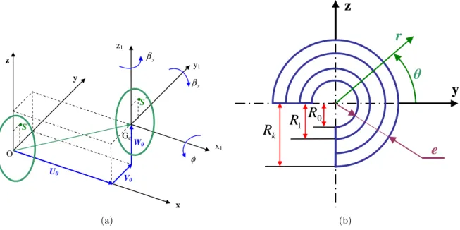
its longitudinal axis. Due to the presence of fibers oriented than axially or circumferentially, coupling is made between bending and twisting. The shaft has a uniform, circular cross section. The following displacement field of a rotating shaft (one beam element) is assumed by choosing the coordinate axisx to coincide with the shaft axis:
⎧⎪⎪⎪ ⎨⎪⎪⎪ ⎩
U(x, y, z, t)=U0(x, t)+zβx(x, t)−yβy(x, t)
V(x, y, z, t)=V0(x, t)−zφ(x, t)
W(x, y, z, t)=W0(x, t)+yφ(x, t)
(1)
Where U,V andW are the flexural displacements of any point on the cross-section of the shaft in the x, y and z directions respectively, the variables U0, V0 and W0 are the flexural displacements of the shaft’s axis, while βx and βy are the rotation angles of the cross-section,
about the y and z axis respectively. The φ is the angular displacement of the cross-section due to the torsion deformation of the shaft (see figure 1).
y z x O Gc y1 x1 y β x β φ z1 U0 V0 W0 S
.
.
S’(a)
y
z
0R
1R
kR
r
e
(b)Figure 1 a) The elastic displacements of a typical cross-section of the shaft, b) k–layers of the composite shaft.
The various components of strain energy of the shaft are presented as follow (one beam element) [6]:
Eda=
1 2A11∫
L
0 (
∂U0 ∂x )
2
dx+12B11[∫
L
0 (
∂βx
∂x)
2
dx+∫0L(
∂βy
∂x)
2
dx]+12ksB66∫
L 0 ( ∂φ ∂x) 2 dx+ 1
2ksA16[2∫
L
0
∂φ ∂x
∂U0 ∂xdx+∫
L
0 βy
∂βx
∂xdx−∫ L
0 βx
∂βy
∂xdx−∫ L
0
∂V0 ∂x
∂βx
∂xdx−∫ L
0
∂W0 ∂x
∂βy
∂xdx]+
1
2ks(A55+A66) [∫
L
0 (
∂V0 ∂x)
2
dx+∫0L(
∂W0 ∂x )
2
dx+∫0Lβ 2
xdx+∫ L
0 β 2
ydx+2∫ L
0 βx
∂W0
∂x dx−2∫ L
0 βy
∂V0 ∂xdx]
Where Aij and Bij are given in Appendix.
The kinetic energy of the rotating composite shaft (one beam element) [6], including the effects of translatory and rotary inertia, can be written as
Eca=
1 2∫
L
0 [ Im(U˙
2 0 +V˙
2 0 +W˙
2
0)+Id(β˙
2
x+β˙
2
y)−2ΩIpβxβ˙y +2ΩIpφ˙+Ipφ˙
2
+
Ω2Ip+Ω2Id(β
2
x+β
2
y)] dx
(3)
where Ω is the rotating speed of the shaft which is assumed constant, L is the length of the shaft, the 2ΩIpβxβ˙y term accounts for the gyroscopic effect, and Id(β˙x2+β˙
2
y) represent
the rotary inertia effect. The mass moments of inertia Im, the diametrical mass moments of
inertia Id and polar mass moment of inertia Ip of rotating shaft per unit length are defined
in the appendix. As the Ω2 Id(β
2
x+β
2
y) term is far smaller than Ω
2
Ip, it will be neglected in
further analysis.
2.2 Kinetic energy of the disk
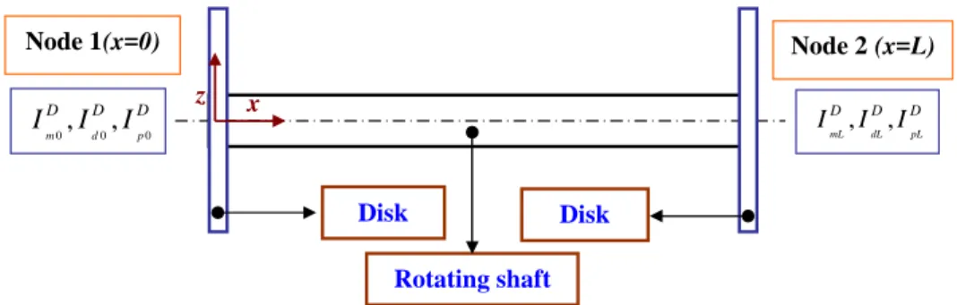
The disk fixed to the composite shaft (see figure 2) is assumed rigid and made of isotropic material. According to Equation (3) the kinetic energy of the disk can be expressed as
EcD=
1 2[I
D m(U˙
2 0 +V˙
2 0 +W˙
2 0)+I
D d (β˙
2
x+β˙
2
y)−2ΩIpDβxβ˙y +2ΩIpDφ˙+IpDφ˙
2
+
Ω2IpD+Ω2IdD(βx2+βy2)]
(4)
where Im, Id and Ip are the mass, the diametrical mass moment of inertia and the polar
mass moment of inertia of the disk. As the Ω2
IpD(βx2+β2y)term is far smaller than Ω
2 IpD, it will be neglected in further analysis.
D D D
p d m I I
I
0 0 0, ,
Node 1(x=0) D D D pL dL mL I I
I , ,
Node 2 (x=L)
Disk
Rotating shaft Disk
x z
Figure 2 Various positions of the disk on the rotating shaft (one element).
2.3 Virtual work of the bearings
The bearings are characterized by values of stiffness and viscous damping following the y and
Rotating shaft
W0 Kyy
Kzz
Kyz
Kzy
Cyy
Czz
Czy C
yz
y z
V0
Figure 3 Model of bearings.
L
x z
zzL zzL
zyL zyL
yzL yzL
yyL yyL
C K
C K
C K
C K
, , , ,
0 0
0 0
0 0
0 0
, , , ,
zz zz
zy zy
yz yz
yy yy
C K
C K
C K
C K
Node 2 (x=L) Node 1(x=0)
Figure 4 Rotating shaft (one element) supported by two bearings.
The virtual work δA done by these external forces can be written as
δA=FV0δV0+FW0δW0 (5)
Where FV0 and Fw0 are the generalized forces expressed by:
{ FV0
FW0
}=−[ Cyy Cyz
Czy Czz ] {
˙ V0
˙
W0 }−[
Kyy Kyz
Kzy Kzz ]{
V0
W0 } (6)
2.4 Hierarchical beam element formulation
The spinning flexible beam is descretised by hierarchical beam elements. Each element with two nodes 1 and 2 is shown in Figure 5. The element’s nodal d.o.f. at each node are U0, V0, W0, βx, βy and φ. The local and non-dimensional co-ordinates are related by
L
L
x
=
ξ
1
2
ξ
,
x
1
=
ξ
0
=
ξ
Figure 5 Beam element with two nodes.
The vector displacement formed by the variables U0 , V0 , W0 , βx , βy and φ can be
written as
⎧⎪⎪⎪⎪ ⎪⎪⎪⎪⎪ ⎪⎪ ⎨⎪⎪⎪ ⎪⎪⎪⎪⎪ ⎪⎪⎪⎩
U0=[NU] {qU}=∑pU
m=1xm(t)⋅fm(ξ) V0=[NV] {qV}=∑pV
m=1ym(t)⋅fm(ξ) W0=[NW] {qW}=∑pW
m=1zm(t)⋅fm(ξ) βx=[Nβx] {qβx}=∑
pβx
m=1βxm(t)⋅fm(ξ)
βy=[Nβy] {qβy}=∑ pβy
m=1βym(t)⋅fm(ξ)
φ=[Nφ] {qφ}=∑pmφ
=1φm(t)⋅fm(ξ)
(8)
where [N] is the matrix of the shape functions, given by
[NU, V, W, βx, βy, φ] =[f1f2. . . fpU, pV, pW, pβx, pβy, pφ] (9)
wherepU , pV , pW , pβx , pβy and pφ are the numbers of hierarchical terms of displacements
(are the numbers of shape functions of displacements). In this work, pU = pV = pW =pβx =
pβy =pφ=p.
The vector of generalized coordinates given by
{q}={qU, qV, qW, qβx, qβy, qφ}T (10)
where
⎧⎪⎪⎪⎪ ⎪⎪⎪⎪⎪ ⎪⎪⎪⎪⎪ ⎪⎨ ⎪⎪⎪⎪⎪ ⎪⎪⎪⎪⎪ ⎪⎪⎪⎪⎪ ⎩
{qU}={x1, x2, x3, ...., xpU} T
exp(jω t) {qV }={y1, y2, y3, ...., ypV}
T
exp(jω t) {qW}={z1, z2, z3, ...., ypW}
T
exp(jω t) {qβx}={βx1, βx2, βx3, ...., βxpβx}
T
exp(jω t) {qβy}={βy1, βy2, βy3, ...., βypβy}
T
exp(jω t) {qφ}={φ1, φ2, φ3, ...., φpφ}
T
exp(jω t)
(11)
⎧⎪⎪⎪⎪ ⎪⎪ ⎨⎪⎪⎪ ⎪⎪⎪⎩
f1=1−ξ
f2=ξ
fr+2=sin(δrξ)
δr =rπ ; r=1, 2, 3, ...
(12)
The functions (f1, f2) are those of the finite element method necessary to describe the nodal displacements of the element; whereas the trigonometric functionsfr+2 contribute only to the internal field of displacement and do not affect nodal displacements. The most attractive particularity of the trigonometric functions is that they offer great numerical stability. The shaft is modeled by elements called hierarchical finite elements withp shape functions for each element. The assembly of these elements is done by theh-version of the finite element method. After modelling the rotating composite shaft using the hp- version of the finite element method and applying the Euler-Lagrange equations, the motion’s equations of free vibration of spinning flexible shaft can be obtained.
[M] {q¨}+[ [G]+[Cp] ] {q˙}+[K] {q}={0} (13)
[M] and [K] are the mass and stiffness matrix respectively,[G] is the gyroscopic matrix and [Cp] is the damping matrix of the bearing (the different matrices of the equation (13) are
given in the appendix).
3 RESULTS
A program based on the formulation proposed to resolve the resolution of the equation (13).
3.1 Convergence
First, the mechanical properties of boron-epoxy are listed in Table 1, and the geometric pa-rameters are L =2.47 m, D =12.69 cm, e = 1.321 mm, 10 layers of equal thickness (90o,
45o,-45o,0o6, 90o). The shear correction factorks =0.503 and the rotating speed Ω =0. In this
example, the boron-epoxy rotating shaft is modeled by one element of length L, then by two elements of equal length L/2.
Table 1 Properties of composite materials [5]. Boron-epoxy Graphite-epoxy
E11 (GPa) 211.0 139.0
E22 (GPa) 24.1 11.0
G12 (GPa) 6.9 6.05
G23 (GPa) 6.9 3.78
ν12 0.36 0.313
ρ (kg/m3
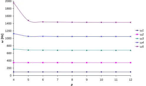
The results of the five bending modes for various boundary conditions of the composite shaft as a function of the number of hierarchical terms p are shown in Figures 6, 7 and 8. Figures clearly show that rapid convergence from above to the exact values occurs when the number of hierarchical terms increased.
The bending modes are the same for a number of hierarchical finite elements, equal 1 then 2. This shows the exactitude of the method even with one element and a reduced number of the shape functions. It is noticeable in the case of low frequencies, a very small p is needed (p=4 sufficient), whereas in the case of the high frequencies, and in order to have a good convergence, p should be increased.
0 200 400 600 800 1000 1200 1400 1600 1800 2000
4 5 6 7 8 9 10 11 12
p
[
H
z
]
1 2 3 4 5
Figure 6 Convergence of the frequencyωfor the 5 bending modes of the simply supported- simply supported
(S-S) shaft as a function of the number of hierarchical termsp.
3.2 Validation
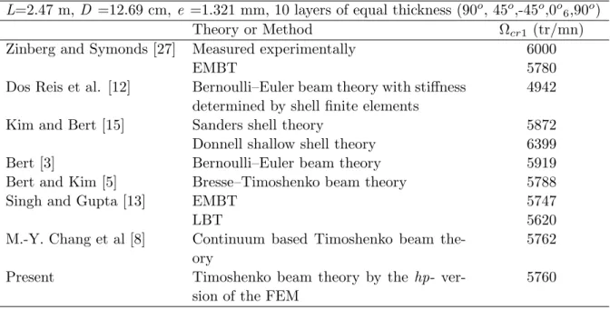
In the following example, the critical speeds of composite shaft are analyzed and compared with those available in the literature to verify the present model. In this example, the composite hollow shafts made of boron-epoxy laminae, which are considered by Bert and Kim [5], are investigated. The properties of material are listed in Table 1. The shaft has a total length of 2.47 m. The mean diameter D and the wall thickness of the shaft are 12.69 cm and 1.321 mm respectively. The lay-up is [90o/45o/-45o/0o6/90o] starting from the inside surface of the
hollow shaft. A shear correction factor of 0.503 is also used. The shaft is modeled by one element. The shaft is simply-supported at the ends. In this validation, p =10.
0 200 400 600 800 1000 1200 1400 1600 1800 2000
4 5 6 7 8 9 10 11 12
p
[H
z
]
1 2 3 4 5
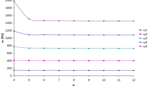
Figure 7 Convergence of the frequencyωfor the 5 bending modes of the clamped-clamped (C-C) shaft as a
function of the number of hierarchical termsp.
0 200 400 600 800 1000 1200 1400 1600 1800 2000
4 5 6 7 8 9 10 11 12
p
[
H
z
]
1 2 3 4 5
Figure 8 Convergence of the frequencyωfor the 5 bending modes of the clamped-supported (C-S) shaft as a
function of the number of hierarchical terms p.
using the Sander shell theory while overestimated by the Donnell shallow shell theory. In this case, the result from the present model is compatible to that of the Continuum based Timoshenko beam theory of M-Y. Chang et al [8]. In this reference the supports are flexible but in our application the supports are rigid.
the advantage of the method used. One should stress here that the present model is not only applicable to the thin-walled composite shafts as studied above, but also to the thick-walled shafts as well as to the solid ones.
Table 2 The first critical speed of the boron-epoxy composite shaft.
L=2.47 m, D =12.69 cm, e =1.321 mm, 10 layers of equal thickness (90o, 45o,-45o,0o6,90o)
Theory or Method Ωcr1 (tr/mn)
Zinberg and Symonds [27] Measured experimentally 6000
EMBT 5780
Dos Reis et al. [12] Bernoulli–Euler beam theory with stiffness determined by shell finite elements
4942
Kim and Bert [15] Sanders shell theory 5872
Donnell shallow shell theory 6399
Bert [3] Bernoulli–Euler beam theory 5919
Bert and Kim [5] Bresse–Timoshenko beam theory 5788
Singh and Gupta [13] EMBT 5747
LBT 5620
M.-Y. Chang et al [8] Continuum based Timoshenko beam the-ory
5762
Present Timoshenko beam theory by the hp-
ver-sion of the FEM
5760
The first eigen-frequency of the boron-epoxy rotating shaft calculated by our program in the stationary case (the rotating speed is null) is 96.0594 Hz on rigid supports and 96.0575 on two elastic supports of stiffness 1740 GN/m. In the reference [9], they used the shell’s theory for the same shaft studied in our case and on rigid supports; the frequency is 96 Hz. In this example, is not noticeable the difference between shaft bi-supported on rigid supports or elastic supports because the stiffness of the supports are very large.
3.3 Results and interpretations
In this study, the results obtained for various applications are presented. Convergence towards the exact solutions is studied by increasing the numbers of hierarchical shape functions for two elements. The influence of the mechanical and geometrical parameters and the boundary conditions on the eigen-frequencies and the critical speeds of the embarked rotating composite shafts are studied. In this study, p = 10
3.3.1 Influence of the gyroscopic effect on the eigen-frequencies
In the following example, the frequencies of a graphite- epoxy rotating shaft are analyzed. The mechanical properties of shaft are shown in Table 1, with ks = 0.503. The ply angles in the
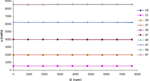
Campbell diagram, for the first five pairs of bending whirling modes of the rotating composite shaft bi-simply supported (S-S) is shown in figure 9. The intersection point of the line (Ω =ω)
with the bending frequency curves, indicate the speed at which the shaft will vibrate violently (i.e., the critical speed Ωcr). The first 10 eigen-values correspond to 5 forward (F) and 5
backward (B) whirling bending modes of the shaft.
Figure 10 shows the variation of the bending fundamental frequency ω as a function of rotating speed Ω (Campbell diagram) for different boundary conditions. The gyroscopic effect inherent to rotating structures induces a precession motion. When the rotating speed increase, the forward modes (1F) increase, whereas the backward modes (1B) decrease.
The gyroscopic effect causes a coupling of orthogonal displacements to the axis of rotation, and by consequence separate the frequencies in two branches: backward precession mode and forward precession mode. In all cases, the forward modes increase with increasing rotating speed however the backward modes decrease.
0 1000 2000 3000 4000 5000 6000 7000 8000 9000
0 1000 2000 3000 4000 5000 6000 7000 8000
[rpm ]
[
ra
d
/s
]
1B
1F
2B
2F
3B
3F
4B
4F
5B
5F
Figure 9 The Campbell Diagram of a graphite- epoxy shaft ((F) forward modes, (B) backward modes).
3.3.2 Influence of the boundary conditions on the eigen-frequencies
In the following example, the boron-epoxy shaft is modeled by two elements of equal length
L/2. The frequencies of the rotating shaft are analyzed. The mechanical properties of shaft are shown in table 1, withks = 0.503. The ply angles in the various layers and the geometrical
400 500 600 700 800 900 1000 1100 1200 1300
0 10000 20000 30000 40000 50000 60000 70000 80000 90000 100000
[rpm]
[
ra
d
/s
]
1B (S-S) 1F (S-S) 1B (C-C) 1F (C-C) 1B (C-S) 1F (C-S) 1B (C-F) 1F (C-F)
Figure 10 The first backward (1B) and forward (1F) bending mode of a graphite- epoxy shaft for different boundary conditions and different rotating speeds (S: simply-supported; C: clamped; F: free).
0 500 1000 1500 2000 2500 3000 3500
0 10000 20000 30000 40000 50000 60000 70000 80000 90000 100000
[rpm]
[
ra
d
/s
]
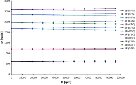
1B (SFS) 1F (SFS) 1B (SSS) 1F (SSS) 1B (CFC) 1F (CFC) 1B (CSC) 1F (CSC) 1B (CSF) 1F (CSF) 1B (SSF) 1F (SSF)
Figure 11 The first backward (1B) and forward (1F) bending mode of a boron- epoxy shaft for different boundary conditions and different rotating speeds. L =2.47 m, D =12.69 cm, e =1.321 mm, 10 layers of equal thickness (90o
, 45o
,-45o
,0o
6, 90o).
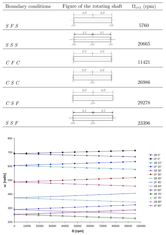
3.3.3 Influence of the lamination angle on the eigen-frequencies
Table 3 The first critical speed of the boron- epoxy shaft for different boundary conditions. Boundary conditions Figure of the rotating shaft Ωcr1 (rpm)
S F S 5760
S S S 20665
C F C 11421
C S C 26986
C S F 29278
S S F 23396
200 300 400 500 600 700 800
0 10000 20000 30000 40000 50000 60000 70000 80000 90000 100000
[rpm]
[r
a
d
/s
]
1B 0° 1F 0° 1B 15° 1F 15° 1B 30° 1F 30° 1B 45° 1F 45° 1B 60° 1F 60° 1B 75° 1F 75° 1B 90° 1F 90°
3.3.4 Influence of the ratios L/D, e/D andη on the critical speeds and rigidity
In figure 13, the first critical speeds of the graphite-epoxy composite shaft (the properties are listed in Table 1, with ks =0.503) are plotted according to the lamination angle for various
ratiosL/D and various boundary conditions (S-S, C-C). From figure 13, the first critical speed of shaft bi-simply supported (S-S) has the maximum value at η = 0o for a ratioL/D = 10, 15
and 20, and at η = 15o for a ratio L/D = 5. For the case of a shaft bi-clamped (C-C), the
maximum critical speed is atη = 0o for a ratio L/D = 20 and at η = 15o for a ratio L/D =
10 and 15, and atη = 30o for a ratioL/D = 5. In figure 14, the second critical speeds of the
same graphite-epoxy composite shaft are plotted according to the lamination angle for various ratios L/D and various boundary conditions (S-S, C-C). From figure 14, the second critical speed for a shaft bi-simply supported has the maximum value at η = 0o for a ratio L/D = 15
and 20, at η = 15o for a ratio L/D = 10 and at η = 30o for a ratio L/D = 5. For the case
of a shaft bi-clamped, the maximum critical speed is atη = 15o for a ratio L/D = 15 and 20,
and at η = 30o for a ratioL/D = 5 and 10.
Above results can be explained as follows. The bending rigidity reaches maximum at η = 0o and reduces when the lamination angle increases; in addition, the shear rigidity reaches
maximum at η = 30o and minimum with η = 0o and η = 90o. A situation in which the
bending rigidity effect predominates causes the maximum to beη = 0o. However, as described by Singh ad Gupta [21], the maximum value shifts toward a higher lamination angle when the shear rigidity effect increases. Therefore, while comparing the phenomena of figure 13 and 14, the constraint from boundary conditions would raise the rigidity effect. A similar is observed for short shafts.
0 10000 20000 30000 40000 50000 60000 70000 80000 90000
0 15 30 45 60 75 90
[°]
1
c
r
[r
p
m
]
L/D=5; S-S L/D=10; S-S L/D=15; S-S L/D=20; S-S L/D=5; C-C L/D=10;C-C L/D=15; C-C L/D=20;C-C
Figure 13 The first critical speed Ω1cr of rotating composite shaft according to the lamination angleη for
0 20000 40000 60000 80000 100000 120000 140000 160000 180000
0 15 30 45 60 75 90
[°]
2
c
r
[
rp
m
]
L/D=5; S-S L/D=10; S-S L/D=15; S-S L/D=20; S-S L/D=5; C-C L/D=10; C-C L/D=15; C-C L/D=20; C-C
Figure 14 The second critical speedΩ2crof rotating composite shaft according to the lamination anglesηfor
various ratiosL/Dand various boundary conditions (S-S, C-C).
In figures 15, 16, 17 and 18, the first and second critical speeds according to ratio L/D of the same graphite-epoxy shaft bi-simply supported (S-S) and the same graphite-epoxy shaft bi- clamped (C-C) for various lamination angles. It is noticeable, if ratio L/D increases, the critical speed decreases and vice versa. Figures 19 and 20 plots the variation of first and second critical speeds successively of the same graphite-epoxy composite shaft with ratio L/D = 20 according to the lamination angle for various e/D ratios and various boundary conditions. It is noticed the influence of the e/D ratio on the critical speed is almost negligible; the curves are almost identical for the variouse/D ratios of each boundary condition. In figures 21, 22, 23 and 24, the same remark is observed; in spite of the variation of the ratio e/D, the critical speed is slightly increased. This is due to the deformation of the cross section is negligible, and thus the critical speed of the thin-walled shaft would approximately independent of thickness ratioe/D.
According to above results, while predicting which stacking sequence of the rotating com-posite shaft having the maximum critical speed, we should consider L/D ratio and the type of the boundary conditions. I.e., the maximum critical speed of a rotating composite shaft is not forever at ply angle equalizes zero degree, but it depends on the L/D ratio and the type the boundary conditions.
Figures 25 and 26 plots the variation of first and second critical speeds successively of the same graphite- epoxy composite shaft with various ply angles, and a rotating steel shaft (E = 207 GPa, G = 79.6 GPa, ν = 0.3, ρ = 7680 kg/m3
0 10000 20000 30000 40000 50000 60000
5 10 15 20
L/D
1
c
r
[
rp
m
]
=0° =15° =30° =45° =60° =75° =90°
Figure 15 The first critical speedΩ1cr of rotating composite shaft bi- simply supported (S-S) according to
ratioL/D for various lamination anglesη.
0 20000 40000 60000 80000 100000 120000 140000 160000
5 10 15 20
L/D
2
c
r
[
rp
m
]
=0° =15° =30° =45° =60° =75° =90°
Figure 16 The second critical speedΩ2crof rotating composite shaft bi- simply supported (S-S) according to
0 10000 20000 30000 40000 50000 60000 70000 80000 90000
5 10 15 20
L/D
1
c
r
[
rp
m
]
=0° =15° =30° =45° =60° =75° =90°
Figure 17 The first critical speedΩ1crof rotating composite shaft bi- clamped (C-C) according to ratioL/D
for various lamination anglesη.
0 20000 40000 60000 80000 100000 120000 140000 160000 180000
5 10 15 20
L/D
2
c
r
[
rp
m
]
=0° =15° =30° =45° =60° =75° =90°
Figure 18 The second critical speedΩ2cr of rotating composite shaft bi- clamped (C-C) according to ratio
0 2000 4000 6000 8000 10000 12000
0 15 30 45 60 75 90
[°]
1
c
r
[
rp
m
]
e/D=0,02; S-S e/D=0,04; S-S e/D=0,06; S-S e/D=0,08; S-S e/D=0,02; C-C e/D=0,04; C-C e/D=0,06; C-C e/D=0,08; C-C
Figure 19 The first critical speed Ω1cr of rotating composite shaft according to the lamination angleη for
various ratiose/Dand various boundary conditions (S-S, C-C).
0 5000 10000 15000 20000 25000 30000
0 15 30 45 60 75 90
[°]
2
c
r
[
rp
m
]
e/D=0,02; S-S e/D=0,04; S-S e/D=0,06; S-S e/D=0,08; S-S e/D=0,02; C-C e/D=0,04; C-C e/D=0,06; C-C e/D=0,08; C-C
Figure 20 The second critical speedΩ2crof rotating composite shaft according to the lamination anglesηfor
1000 2000 3000 4000 5000 6000
0,02 0,04 0,06 0,08
e/D
1
c
r
[
rp
m
]
=0° =15° =30° =45° =60° =75° =90°
Figure 21 The first critical speedΩ1cr of rotating composite shaft bi- simply supported (S-S) according to
ratioe/Dfor various lamination anglesη(L/D=20).
5000 10000 15000 20000
0,02 0,04 0,06 0,08
e/D
2
c
r
[
rp
m
]
=0° =15° =30° =45° =60° =75° =90°
Figure 22 The second critical speedΩ2crof rotating composite shaft bi- simply supported (S-S) according to
2000 4000 6000 8000 10000 12000
0,02 0,04 0,06 0,08
e/D
1
c
r
[
rp
m
]
=0° =15° =30° =45° =60° =75° =90°
Figure 23 The first critical speedΩ1cr of rotating composite shaft bi- clamped (C-C) according to ratioe/D
for various lamination anglesη(L/D=20).
8000 10000 12000 14000 16000 18000 20000 22000 24000 26000
0,02 0,04 0,06 0,08
e/D
2
c
r
[
rp
m
]
=0° =15° =30° =45° =60° =75° =90°
Figure 24 The second critical speedΩ2cr of rotating composite shaft bi- clamped (C-C) according to ratio
(S-S), the same first or second critical speed for a composite shaft with a lamination angle η = 30o, a steel shaft is needed for a length lower than that of the composite shaft. The steel
shaft bi- clamped (C-C) has the highest first critical speed when LID is less than 7.5. The case where L/D between 7.5 and 20, the first critical speed with η =30o is largest that the others. In figures 27 and 28, in spite of the change of the e/D ratio, the critical speed is slightly increased. This is due to the deformation of the cross section is negligible, and thus the critical speed of the thin-walled shaft would approximately independent of thickness ratio e/D. The critical speeds of steel shaft are between those of the composite shaft which have successively the lamination angles 30o and 60o.
0 20000 40000 60000 80000 100000 120000 140000 160000
5 10 15 20
L/D
c
r
[
rp
m
]
1cr (steel) 2cr (steel) 1cr ( =30°) 2cr ( =30°) 1cr ( =60°) 2cr ( =60°)
Figure 25 The first and second critical speed of rotating composite shaft for various lamination angles, and rotating steel shaft, bi- simply supported (S-S) according to ratioL/D.
3.3.5 Influence of the stacking sequence on the eigen-frequencies
In order to show the effects of the stacking sequence on the eigen-frequencies, a rotating carbon-epoxy shaft is mounted on two rigid supports; the mechanical and geometrical properties of this shaft are [22]:
E11 = 130 GPa, E22 = 10 GPa,G12 = G23 = 7 GPa, ν12 = 0.25,ρ = 1500 Kg/m3
L =1.0 m,D = 0.1 m, e = 4 mm, 4 layers of equal thickness, ks = 0.503
A four-layered scheme was considered with two layers of 0o and two of 90o fibre angle.
The flexural frequencies have been obtained for different combinations (both symmetric and unsymmetric) of 0o and 90o orientations (see figures 29 and 30). These figures, respectively
0 20000 40000 60000 80000 100000 120000 140000 160000 180000
5 10 15 20
L/D
c
r
[
rp
m
]
1cr (steel) 2cr (steel) 1cr ( =30°) 2cr ( =30°) 1cr ( =60°) 2cr ( =60°)
Figure 26 The first and second critical speed of rotating composite shaft for various lamination angles, and rotating steel shaft, bi- clamped (C-C) according to ratioL/D.
0 2000 4000 6000 8000 10000 12000 14000 16000
0,02 0,04 0,06 0,08
e/D
c
r
[
rp
m
] 1cr (steel)2cr (steel)
1cr ( =30°) 2cr ( =30°) 1cr ( =60°) 2cr ( =60°)
0 5000 10000 15000 20000 25000
0,02 0,04 0,06 0,08
e/D
c
r
[
rp
m
]
1cr (steel) 2cr (steel) 1cr ( =30°) 2cr ( =30°) 1cr ( =60°) 2cr ( =60°)
Figure 28 The first and second critical speed of rotating composite shaft for various lamination angles, and rotating steel shaft, bi- clamped (C-C) according to ratioe/D (L/D=20).
315 320 325 330 335 340 345 350 355 360 365
0 10000 20000 30000 40000 50000 60000 70000 80000 90000 100000
[rpm]
1
[
H
z
]
1B (90°,90°,0°,0°)
1F (90°,90°,0°,0°)
1B (0°,0°,90°,90°)
1F (0°,0°,90°,90°)
1B (0°,90°,90°,0°)
1F (0°,90°,90°,0°)
1B (90°,0°,0°,90°)
1F (90°,0°,0°,90°)
1B (0°,90°,0°,90°)
1F (0°,90°,0°,90°)
1B (90°,0°,90°,0°)
1F (90°,0°,90°,0°)
1030 1040 1050 1060 1070 1080 1090 1100 1110
0 10000 20000 30000 40000 50000 60000 70000 80000 90000 100000
[rpm]
2
[
H
z
]
2B (90°,90°,0°,0°)
2F (90°,90°,0°,0°)
2B (0°,0°,90°,90°)
2F (0°,0°,90°,90°)
2B (0°,90°,90°,0°)
2F (0°,90°,90°,0°)
2B (90°,0°,90°,0°)
2F (90°,0°,90°,0°)
2B (90°,0°,0°,90°)
2F (90°,0°,0°,90°)
2B (90°,0°,90°,0°)
2F (90°,0°,90°,0°)
Figure 30 Second bending eigen-frequency of the rotating carbon- epoxy shaft bi- simply supported (S-S) for stacking sequences according to the rotating speed.
configurations, the frequency values of the rotating composite shaft are very close, and does have a slight dependence on the relative positioning of the 0o and 90o layers.
3.3.6 Influence of the disk’s position according to the rotating shaft on on the eigen-frequencies
This part begins with a validation in the case of a stationary embarked shaft bi- simply supported (the rigid disk at the mid-span), the mechanical and geometrical properties of the shaft and the steel disk are as follows: E = 207 GPa, ν = 0.3,ρ = 7800 kg/m3
• Shaft: Length = 457 mm, Interior ray = 12.7 mm, External ray = 17.7 mm.
• Disk: External ray = 88.5 mm; Thickness = 4.425 mm.
The first frequency of the system (shaft + disk) calculated by our program in the stationary case (the rotating speed is null) is 310 Hz on rigid support (with ks=0.56). In the reference
[17] they used a thick three-dimensional cylindrical element by applying the theory 3D for the same shaft studied in our case but with a flexible disk, the found frequency is 288 Hz. In this application, is noticeable the difference between the two works because the various theories applied, and the flexibility of the disk.
Disk
Rotating shaft x
L
Figure 31 System; embarked hollow rotating shaft.
The Campbell diagram containing the frequencies of the second pairs of bending whirling modes of the above composite system is shown in figure 32. Denote the ratio of the whirling bending frequency and the rotation speed of shaft as γ. The intersection point of the line (γ=1) with the whirling frequency curves indicate the speed at which the shaft will vibrate violently (i.e., the critical speed). In figure 32 the second pair of the forward and backward whirling frequencies falls more wide apart in contrast to other pairs of whirling modes. This might be due to the coupling of the pitching motion of the disk with the transverse vibration of shaft. Note that the disk is located at the mid-span of the shaft, while the second whirling forward and backward bending modes are skew-symmetric with respect to the mid-span of the shaft. The size of the curve of the first pairs of the bending frequencies is increased in order to view better (see figure 33). Figure 34 shows the Campbell diagram of the first two bending frequencies of the embarked graphite- epoxy shaft for various disk’s positions (x) according to the shaft (see figure 31). It is noted that when the disk approaches the support, the first bending frequency decreases and the second bending frequency increases and vice versa.
Table 4 Properties of the system (shaft + disk).
Properties Shaft Disk
L (m) 0.72
Interior ray (m) 0.028 External ray (m) 0.048
ks 0.56
Im (kg) 2.4364
Id (kg m
2
) 0.1901
Ip (kg m
2
) 0.3778
3.3.7 Influence of the geometrical form of the rotating shaft on the eigen-frequencies
0 500 1000 1500 2000 2500 3000
0 1000 2000 3000 4000 5000 6000 7000 8000 9000 10000
[rpm]
[
ra
d
/s
] 1B
1F 2B 2F =1
Figure 32 Campbell diagram of the first two bending frequencies of the embarked graphite-epoxy shaft.
941,6 941,8 942 942,2 942,4 942,6 942,8 943 943,2
0 1000 2000 3000 4000 5000 6000 7000 8000 9000 10000
[rpm]
1
[
ra
d
/s
]
1B 1F
0 500 1000 1500 2000 2500 3000 3500 4000
0 1000 2000 3000 4000 5000 6000 7000 8000 9000 10000
[rpm]
[
ra
d
/s
]
1B (x=L/2)
1F (x=L/2) 2B (x=L/2) 2F (x=L/2) 1B (x=L/4) 1F (x=L/4) 2B (x=L/4)
2F (x=L/4) 1B (x=L/8) 1F (x=L/8) 2B (x=L/8) 2F (x=L/8)
Figure 34 Campbell diagram of the first two bending frequencies of the graphite-epoxy shaft for various disk’s positions (x) according to the shaft.
and staged) are given by table 5. The properties of a uniform rigid disk are listed in table 4. The disk is placed at the free end of the shaft. Figure 35 shows the studied systems. For the finite element analysis, the shaft is modeled into two elements of equal lengths. The first element (Stage 1) is bi-simply supported (S-S) and the second element (Stage 2) is simply supported - free (S-F). The disk is placed at the free boundary (F). Figure 36 shows the Campbell diagram of the first two bending frequencies of the systems; embarked graphite-epoxy shaft for the various geometrical forms of the shaft (see figure 35).
It is noted that the eigen-frequencies in the case of a shaft not staged are lower than those of a staged shaft.
Table 5 Geometrical properties of the rotating shafts.
Dimension
Staged shaft
Not staged shaft
Stage 1 Stage 2
L(m) 0.360 0.360 0.720
D (m) 0.048 0.038 0.038
e (m) 0.020 0.010 0.010
Numbers layers (with equal thick-nesses)
20 10 10
η (o) 90o, 45o,-45o,0o6,
90o, 90o,
45o,-45o,0o6, 90o
Stage 1 Stage 2
Disk
(a) Staged embarked rotating shaft
Rotating shaft
Disk
(b) Not staged embarked rotating shaft
Figure 35 System; embarked hollow rotating shaft.
0 1000 2000 3000 4000 5000 6000
0 1000 2000 3000 4000 5000 6000 7000 8000 9000 10000
[rpm]
[
ra
d
/s
]
1B (not staged) 1F (not staged) 2B (not staged) 2F (not staged) 1B (staged) 1F (staged) 2B (staged) 2F (staged)
4 CONCLUSION
The analysis of the free vibrations of the rotating composite shafts using thehp-version (hierar-chical finite element method (p-version) with trigonometric shape functions combined with the standard finite element method (h-version)), is presented in this work. The results obtained agree with those available in the literature. Several examples were treated to determine the influence of the various geometrical and physical parameters of the embarked rotating shafts. This work enabled us to arrive at the following conclusions:
1. Monotonous and uniform convergence is checked by increasing the number of the shape functions p, and the number of the hierarchical finite elements. The convergence of the solutions is ensured by the element beam with two nodes. The results agree with the solutions found in the literature.
2. The gyroscopic effect causes a coupling of orthogonal displacements to the axis of ro-tation, and by consequence separates the frequencies in two branches, backward and forward precession modes. In all cases the forward modes increase with increasing rotat-ing speed however the backward modes decrease. This effect has a significant influence on the behaviours of the rotating shafts.
3. The rotating composite shafts must cross several critical speeds in acceleration and de-celeration.
4. The dynamic characteristics and in particular the eigen-frequencies, the critical speeds and the bending and shear rigidity of the rotating composite shafts are influenced appre-ciably by changing the ply angle, the stacking sequence, the length, the mean diameter, the materials, the rotating speed and the boundary conditions.
5. The critical speed of the thin-walled rotating composite shaft is approximately indepen-dent of the thickness ratio and mean diameter of the rotating shaft.
6. The critical speeds of the rotating steel shaft are between those of the rotating composite shafts which have successively the ply angle 30o and 60o.
7. The dynamic characteristics of the system (shaft + disk + support) are influenced ap-preciably by changing disk’s positions according to the the shaft and the section of the shaft.
8. The determination of the dynamic characteristics of the embarked rotating composite shaft of variable sections with various disk’s positions is ensured by our calculation pro-gram.
References
[1] I. Babuˇska, B. A Szab´o, and I. N. Katz. Thep- version of the finite element method. SIAM Journal on Numerical Analysis, 18(515-545), 1981.
[2] N. S. Bardell. The application of symbolic computing to hierarchical finite element method.Int. J. Num. Meth. Eng, 28:1181–1204, 1989.
[3] C. W. Bert. The effect of bending–twisting coupling on the critical speed of a driveshafts. In Proceedings. 6th Japan-US Conference on Composites Materials, pages 29–36, Orlando, FL. Technomic, Lancaster, PA, 1992.
[4] C. W. Bert and C. D. Kim. Dynamic instability of composite-material drive shaft subjected to fluctuating torque and/or rotational speed. Dynamics and Stability of Systems, 2:125–147, 1995.
[5] C. W. Bert and C. D. Kim. Whirling of composite-material driveshafts including bending, twisting coupling and transverse shear deformation.Journal of Vibration and Acoustics, 117(17-21), 1995.
[6] A. Boukhalfa, A. Hadjoui, and S. M. Hamza Cherif. Free vibration analysis of a rotating composite shaft using the
p-version of the finite element method. International Journal of Rotating Machinery, page 10, 2008. Article ID 752062.
[7] C. Y. Chang et al. Vibration analysis of rotating composite shafts containing randomly oriented reinforcements.
Composite structures, 63:21–32, 2004.
[8] M. Y. Chang et al. A simple spinning laminated composite shaft model. International Journal of Solids and Structures, 41:637–662, 2004.
[9] E. Chatelet et al. A three dimensional modeling of the dynamic behavior of composite rotors. International Journal of Rotating Machinery, 8(3):185–192, 2002.
[10] L. W. Chen and W. K. Peng. The stability behaviour of rotating composite shafts under axial compressive loads.
Composite Structures, 41:253–263, 1998.
[11] A. Cot´e and F. Charron. On the selection ofp- version shape functions for plate vibration problems. Computers and Structures, 79:119–130, 2001.
[12] H. L. M. Dos Reis, R. B. Goldman, and P. H. Verstrate. Thin walled laminated composite cylindrical tubes: Part III – critical speed analysis.Journal of Composites Technology and Research, 9:58–62, 1987.
[13] K. Gupta and S. E. Singh. Dynamics of composite rotors. InProceedings of Indo-US symposium on Emerging Trends in Vibration and Noise Engineering, pages 59–70, New Delhi, India, 1996.
[14] A. Houmat. A sector fourierp- element applied to free vibration analysis of sector plates. Journal of Sound and Vibration, 243:269–282, 2001.
[15] C. D. Kim and C. W. Bert. Critical speed analysis of laminated composite. hollow drive shafts. Composites Engi-neering, 3(633-643), 1993.
[16] L. Meirovitch and H. Baruh. On the inclusion principle for the hierarchical finite element method. Int. J. Num. Meth. Eng, 19:281–291, 1983.
[17] A. A. S. Shahab and J. Thomas. Coupling effects of disc flexibility on the dynamic behaviour of multi disc-shaft systems. Journal of Sound and Vibration, 114(3):435–452, 1987.
[18] S. E. Singh and K. Gupta. Experimental studies on composite shafts. InProceedings of the International Conference on Advances in Mechanical Engineering, pages 1205–1221, Bangalore, India, 1995.
[19] S. P. Singh.Some Studies on Dynamics of Composite Shafts. PhD thesis, Mechanical Engineering Department, IIT, Delhi, India, 1992.
[20] S. P. Singh and K. Gupta. Dynamic analysis of composite rotors. In 5th International Symposium on Rotating Machinery (ISROMAC-5), also International Journal of Rotating Machinery, pages 179–186, 2, 1994.
[21] S. P. Singh and K. Gupta. Free damped flexural vibration analysis of composite cylindrical tubes using beam and shell theories.Journal of Sound and Vibration, 172:171–190, 1994.
[22] S. P. Singh and K. Gupta. Composite shaft rotordynamic analysis using a layerwise theory. Journal of Sound and Vibration, 191(5):739–756, 1996.
[24] B. A. Szab´o and G. J. Sahrmann. Hierarchical plate and shells models based on p-extension. Int. J. Num. Meth. Eng., 26:1855–1881, 1988.
[25] H. L. Wettergren. Delamination in composite rotors.Composites Part A, 28A:523–527, 1997.
[26] D. C. Zhu. Development of hierarchical finite element method at biaa. InProc. of the International Conference on Computational Mechanics, volume I, pages 123–128, Tokyo, 1986.
APPENDIX
The termsAij,Bij of the equation (2) andIm,Id,Ip of the equation (3) are given as follows:
⎧⎪⎪⎪⎪ ⎪⎪⎪⎪⎪ ⎪⎪ ⎨⎪⎪⎪ ⎪⎪⎪⎪⎪ ⎪⎪⎪⎩
A11=π∑kn
=0C
′
11n(R
2
n+1−R 2
n)
A55=π
2∑
k n=0C
′
55n(R
2
n+1−R 2
n)
A66=π
2∑
k n=0C
′
66n(R 2
n+1−R 2
n)
A16=2π
3 ∑
k n=0C
′
16n(R
3
n+1−R 3
n)
B11= π
4∑
k n=0C
′
11n(R
4
n+1−R 4
n)
B66=π
2∑
k n=0C
′
66n(R 4
n+1−R 4 n) (A1a) ⎧⎪⎪⎪⎪ ⎨⎪⎪⎪ ⎪⎩
Im=π∑kn=0 ρn(R 2
n+1−R 2
n)
Id= π4∑
k
n=0 ρn(R 4
n+1−R 4
n)
Ip= π2∑
k
n=0 ρn(R 4
n+1−R 4
n)
(A1b)
Where k is the number of the layer, Rn−1 is the nth layer inner radius of the composite shaft andRn it is thenth layer outer of the composite shaft. Lis the length of the composite
shaft and ρn is the density of thenth layer of the composite shaft.
The indices used in the matrix forms are as follows:
a: shaft;D: disk; e: element;P: bearing (support)
The various matrices of the equation (13) which assemble the elementary matrices of the system as follows:
Shaft
[Mae]=
⎡⎢ ⎢⎢ ⎢⎢ ⎢⎢ ⎢⎢ ⎢⎢ ⎢⎣
[MU] 0 0 0 0 0
0 [MV] 0 0 0 0
0 0 [MW] 0 0 0
0 0 0 [Mβx] 0 0
0 0 0 0 [Mβy] 0
0 0 0 0 0 [Mφ]
⎤⎥ ⎥⎥ ⎥⎥ ⎥⎥ ⎥⎥ ⎥⎥ ⎥⎦ (A2)
[Kae]=
⎡⎢ ⎢⎢ ⎢⎢ ⎢⎢ ⎢⎢ ⎢⎢ ⎢⎢ ⎣
[KU] 0 0 0 0 [K1]
0 [KV] 0 [K2] [K3] 0
0 0 [KW] [K4] [K5] 0
0 [K2]T [K4]T [Kβx] [K6] 0
0 [K3]T [K5]T [K6]T [Kβy] 0
[K1]T 0 0 0 0 [Kφ]
[Gea]= ⎡⎢ ⎢⎢ ⎢⎢ ⎢⎢ ⎢⎢ ⎢⎢ ⎢⎣
0 0 0 0 0 0
0 0 0 0 0 0
0 0 0 0 0 0
0 0 0 0 [G1] 0
0 0 0 −[G1]T 0 0
0 0 0 0 0 0
⎤⎥ ⎥⎥ ⎥⎥ ⎥⎥ ⎥⎥ ⎥⎥ ⎥⎦ (A4)
[MU]=ImL∫
1 0 [
NU]T[NU] dξ (A5a)
[MV]=ImL∫
1 0 [
NV]T[NV] dξ (A5b)
[MW]=ImL∫
1 0 [
NW]T[NW] dξ (A5c)
[Mβx]=IdL∫
1 0 [
Nβx]T[Nβx] dξ (A5d)
[Mβy]=IdL∫
1 0 [
Nβy] T
[Nβy] dξ (A5e)
[Mφ]=IpL∫
1 0 [
Nφ]T[Nφ] dξ (A5f)
[KU]=
1 LA11∫
1 0 [N
′ U]
T
[N′
U] dξ (A5g)
[KV]=
1
Lks(A55+A66)∫ 1 0 [
N′ V]
T
[N′
V] dξ (A5h)
[KW]=
1
Lks(A55+A66)∫ 1 0 [
N′ W]
T
[N′
W] dξ (A5i)
[K1]= 1
LksA16∫ 1 0 [
N′ φ]
T
[N′
U] dξ (A5j)
[K2]=− 1
2LksA16∫ 1 0 [
N′ V]
T
[N′
βx] dξ (A5k)
[K3]=−ks(A55+A66)∫
1 0 [Nβy]
T
[N′
V] dξ (A5l)
[K4]=ks(A55+A66)∫
1 0 [
Nβx] T
[N′
W] dξ (A5m)
[K5]=− 1
2LksA16∫ 1 0 [
N′ W]
T
[N′
βy] dξ (A5n)
[K6]=[1
2ksA16∫ 1 0 [
Nβy] T
[N′
βx] dξ]−[
1
2ksA16∫ 1 0 [
Nβx] T[
N′
βy] dξ] (A5o)
[Kβx]=[
1 LB11∫
1 0 [N
′ βx]
T
[N′
βx] dξ]+[Lks(A55+A66)∫
1 0 [Nβx]
T
[Kβy]=[
1 LB11∫
1 0 [
N′ βy]
T
[N′
βy] dξ]+[Lks(A55+A66)∫
1 0 [
Nβy] T
[Nβy] dξ] (A5q)
[Kφ]=
1 LB66∫
1 0 [
N′ φ]
T
[N′
φ] dξ (A5r)
[G1]=ΩIpL∫
1 0 [
Nβx] T
[Nβy] dξ (A5s)
Where [N′ i]=
∂[Ni]
∂ξ , with (i = U, V, W,βx,βy,φ).
Disc
[MDe]=
⎡⎢ ⎢⎢ ⎢⎢ ⎢⎢ ⎢⎢ ⎢⎢ ⎢⎣
[ImD] 0 0 0 0 0
0 [ImD] 0 0 0 0
0 0 [ImD] 0 0 0
0 0 0 [IdD] 0 0
0 0 0 0 [IdD] 0
0 0 0 0 0 [IpD]
⎤⎥ ⎥⎥ ⎥⎥ ⎥⎥ ⎥⎥ ⎥⎥ ⎥⎦ (A6)
[GeD]=
⎡⎢ ⎢⎢ ⎢⎢ ⎢⎢ ⎢⎢ ⎢⎢ ⎢⎢ ⎣
0 0 0 0 0 0
0 0 0 0 0 0
0 0 0 0 0 0
0 0 0 0 Ω[ID
p ] 0
0 0 0 −Ω[IpD] T
0 0
0 0 0 0 0 0
⎤⎥ ⎥⎥ ⎥⎥ ⎥⎥ ⎥⎥ ⎥⎥ ⎥⎥ ⎦ (A7) Bearings
[KPe]=
⎡⎢ ⎢⎢ ⎢⎢ ⎢⎢ ⎢⎢ ⎢⎢ ⎢⎣
0 0 0 0 0 0
0 [Kyy] [Kyz] 0 0 0
0 [Kzy] [Kzz] 0 0 0
0 0 0 0 0 0
0 0 0 0 0 0
0 0 0 0 0 0
⎤⎥ ⎥⎥ ⎥⎥ ⎥⎥ ⎥⎥ ⎥⎥ ⎥⎦ (A8)
[CPe]=
⎡⎢ ⎢⎢ ⎢⎢ ⎢⎢ ⎢⎢ ⎢⎢ ⎢⎣
0 0 0 0 0 0
0 [Cyy] [Cyz] 0 0 0
0 [Czy] [Czz] 0 0 0
0 0 0 0 0 0
0 0 0 0 0 0
0 0 0 0 0 0
⎤⎥ ⎥⎥ ⎥⎥ ⎥⎥ ⎥⎥ ⎥⎥ ⎥⎦ (A9)
⎧⎪⎪⎪⎪ ⎪⎪ ⎨⎪⎪⎪ ⎪⎪⎪⎩
[Me]=[Mae]+[Me D]
[Ge]=[Ge
a]+[GeD]
[Ke]=[Ke
a]+[KPe]
[Ce P]
(A10)
The various matrices (globally matrices) which assemble the elementary matrices, according to the boundary conditions as follows:
⎧⎪⎪⎪⎪ ⎪⎪ ⎨⎪⎪⎪ ⎪⎪⎪⎩
[M]=[Ma]+[MD]
[G]=[Ga]+[GD]
[K]=[Ka]+[KP]
[CP]
(A11)
The terms of the matrices are a function of the integrals: Jm nα β =∫1
0 f
α
m(ξ) fnβ(ξ) dξ (m,