UNIVERSIDADE FEDERAL DO CEARÁ (UFC)
DEPARTAMENTO DE ENGENHARIA DE TRANSPORTES (DET)
PROGRAMA DE PÓS-GRADUAÇÃO EM ENGENHARIA DE TRANSPORTES
(PETRAN)
LUCAS FEITOSA DE ALBUQUERQUE LIMA BABADOPULOS
A CONTRIBUTION TO COUPLE AGING TO HOT MIX ASPHALT (HMA)
MECHANICAL CHARACTERIZATION UNDER LOAD-INDUCED DAMAGE
FORTALEZA
A CONTRIBUTION TO COUPLE AGING TO HOT MIX ASPHALT (HMA)
MECHANICAL CHARACTERIZATION UNDER LOAD-INDUCED DAMAGE
A Thesis submitted as partial fulfillment of the requirements for the Master’s Degree in Transportation Engineering at Universidade Federal do Ceará.
Area within the Graduate Program: Transportation Infrastructure
Advisor: Jorge Barbosa Soares, Ph.D.
Dados Internacionais de Catalogação na Publicação Universidade Federal do Ceará
Biblioteca de Pós-Graduação em Engenharia - BPGE
B111c Babadopulos, Lucas Feitosa de Albuquerque Lima.
A contribution to couple aging to hot mix asphalt (hma) mechanical characterization under load-induced damage / Lucas Feitosa de Albuquerque Lima Babadopulos. – 2014.
139 f. : il., enc. ; 30 cm.
Dissertação (mestrado) – Universidade Federal do Ceará, Centro de Tecnologia, Programa de Pós-Graduação em Engenharia de Transportes, Fortaleza, 2014.
Área de Concentração: Infraestrutura de Transportes. Orientação: Prof. Dr. Jorge Barbosa Soares.
1. Transportes. 2. Mistura asfáltica. 3. Fadiga. 4. Deformação permanente. I. Título.
As this paragraph typically deals with the emotion behind the work that was done, I think it is necessary to write it in the author's mother language. I will write it in Portuguese.
Antes de começar, gostaria de dizer que eu adoro essa seção. Só ela tenta traduzir a emoção por trás de cada trabalho e o justifica, sem precisar argumentar. É aqui que ficam impressas, ainda que como pano de fundo, as razões-emoções que estão afastadas do plano intelectual, mas que acompanham diretamente o autor do trabalho científico. Ainda que o estilo de todo autor apareça veladamente no texto científico, a própria escrita científica faz de tudo para esconder o que o autor é, para que sobressaia o que foi feito por ele, impessoalmente. Ademais, pensar sobre as participações dos outros nessa etapa marcante da minha vida me traz bem estar gratuitamente: mais um motivo pelo qual adoro essa seção.
Primeiro, devo dizer que foi durante o mestrado no Petran que decidi me casar com a Priscilla e partir para o doutorado em Lyon. Sendo assim, de certa forma, o estabelecimento desses passos como parte dos meus planos contribuiu positivamente para minha atitude em terminar bem o mestrado, mas muito mais importante que isso, mudou tudo. Obrigado, Minha Vida, por ter me movido para frente, espero que possamos mover um ao outro para sempre.
departamento eu também devo agradecer pelo aprendizado do dia-a-dia que ele pode trazer. Ademais, foi o ambiente em que amizades especiais e muito distintas foram cativadas. Em especial, o Petran foi o palco de bastante aprendizado cotidiano, sem contar a felicidade que tive em estudar com a maioria de seus professores. A esses sim devo muito agradecimento. Nos bons professores sempre sinto uma esperança de fazer o mundo melhor, usando esse método silencioso e paciente que parece ser ensinar. Não lembro de gostar tanto de uma disciplina quanto da de Estatística com o Manoel... A disciplina da Verônica acabou por render muito trabalho com os companheiros de guerra Juceline, Reuber e Lorran, mas o suor intelectual valeu a pena. Estive especialmente feliz de ver o Prof. Jorge se motivar para plantar a semente do que espero ser a futura disciplina de Viscoelasticidade no Petran, que pode sistematicamente elevar a outros níveis o trabalho de interpretação de resultados no LMP e a formação dos alunos na área de misturas e ligantes asfálticos.
Ao pessoal que possibilita o funcionamento do LMP, sem o qual não haveria nem
esse trabalho nem provavelmente nenhum dos outros de meus colegas. Em especial à Annie e
ao Rômulo (e seus ajudantes), que viram quase tudo que o laboratório já pôde produzir.
Aliás, foi nesse trabalho que o Rômulo bateu seu record de produção diária de corpos-de-prova. Aconteceu na semana anterior à do Natal de 2013, após o início do recesso. Infelizmente prometi guardar o segredo da quantidade de CPs comigo para sempre. Fica aqui o agradecimento pela enorme disposição para terminar o trabalho num tempo tão apertado. Sem aquele esforço em dezembro eu certamente não teria terminado o mestrado em Junho e a partida para o doutorado em Lyon teria sido totalmente desorganizada.
Aos alunos da graduação em Engenharia Civil da UFC Jorge Luís e Cristina. Sem eles o trabalho não teria sido terminado. A experiência de treiná-los no laboratório me ajudou mais do que eles imaginam. Ainda espero que essa ação entre em ressonância com a continuidade do trabalho do Jorge Luís. Boto muita fé que vai ser ele quem sistematizará o treinamento dos novos alunos nas prensas e vai dinamizar bastante a formação no LMP através dos nossos futuros Guias de Treinamento. Esse menino é bom!
incrívis. Que bom que ainda deu certo você aparecer via internet para as discussões do trabalho na defesa!
Um grande agradecimento aos avaliadores externos do trabalho, Prof. Y. Richard
Kim da NCSU/Raleigh e Prof. Thiago Aragão da Coppe/UFRJ. O primeiro é simplesmente
uma das referências internacionais na nossa área de pesquisa, enquanto o segundo é um exemplo especial de "onde podemos chegar" para os alunos do LMP que buscam a carreira acadêmica. É um privilégio e uma grande honra ter de seus ídolos lhe avaliando. Tenho muita sorte! Espero que meu trabalho tenha contribuído para as relações e trabalhos futuros do LMP, cuja camisa visto com tanto gosto desde 2007.
Agradeço também aos financiadores de pesquisa no Brasil, em especial ao que tocou diretamente esse trabalho, o CNPq, através da minha bolsa de mestrado e do Projeto Universal/CNPq do Prof. Jorge, que lida com caracterização viscoelastoplástica de misturas asfálticas, no qual estou inserido. Sem esse tipo de financiamento, pesquisas com teor mais fundamental dificilmente poderiam ser conduzidas e a ciência no Brasil veria seus próprios problemas ficarem "atrasados" ao longo do tempo, imagine suas soluções. Ainda bem que isso existe.
Deixei o maior agradecimento para o final e ele acaba estando na origem de tudo:
os Pais. Esse agradecimento é estendido aos pais dos pais e aos pais deles, e no fundo, à
Although aging simulation in binder is performed through RTFO and PAV tests, no considerations of asphalt mixture aging are made in regular laboratory characterization. The present work is focused in incorporating aging to the modeling of the mechanical behavior of hot mix asphalt (HMA) during load-induced damage. This is accomplished by combining existing models and the adaptation of mixture aging procedures. The aging model used is based on the evolution of an internal state variable, associated to oxygen availability, aging temperature and four material parameters. These parameters are related to aging susceptibility, reaction kinetics and dependency on aging history and on aging temperature. The model allows to establish relationships between different aging processes. Results at four aging states (using two different temperatures) were analyzed and the aging model parameters were estimated. Capturing aging dependency on temperature constitutes a contribution of the present work with respect to previous results reported in the literature. The aging model is coupled to viscoplasticity and damage, comparing the behavior observed at the different aging states. Concerning the damage models, this thesis used mechanical models derived from Schapery's work potential theory to model fatigue behavior. The Simplified Viscoelastic Continuum Damage (S-VECD) model was selected. Unconfined dynamic creep tests were used to evaluate the effect of aging in the mixture resistance to permanent deformation. In addition to the state-of-the-art modeling of HMA, the characterization methods currently in use in Brazil (tensile strength, resilient modulus and controlled force indirect tensile fatigue tests) were also conducted. The possibility to simulate the material behavior for various loading conditions constitutes an advantage of the state-of-the-art model over the state-of-the practice method for fatigue characterization, used primarily to rank mixtures. It was concluded that, depending on pavement conditions and layer geometry, aging not necessarily affects negatively the fatigue behavior, while certainly improving the permanent deformation characteristics. That happens despite the fact that aging produces less damage tolerant materials, i.e., materials that fail for less evolved damage states. The framework (testing and analysis) for damage characterization of asphalt mixtures was implemented and it is expected to contribute to further developments in aging modeling of asphalt mixtures.
Apesar de simulação de envelhecimento ser realizada em ligantes asfálticos através dos ensaios de RTFOT e PAV, nenhuma consideração sobre envelhecimento de misturas é feita na caracterização laboratorial comum. O presente trabalho se concentra na incorporação do envelhecimento na modelagem do comportamento mecânico de concretos asfálticos (CA) para carregamentos que induzem dano. Isto é feito através da combinação de modelos e da adaptação de procedimentos de envelhecimento existentes. O modelo de envelhecimento utilizado se baseia na evolução de uma variável interna de estado e é associado à disponibilidade de oxigênio, à temperatura e a quatro parâmetros materiais. Estes parâmetros são relacionados à susceptibilidade ao envelhecimento, à cinética de reação e à dependência sobre o histórico e sobre a temperatura de envelhecimento. O modelo permite estabelecer relações entre diferentes processos de envelhecimento. Resultados em quatro estados de envelhecimento (em duas temperaturas diferentes) foram analisados, e os parâmetros do modelo estimados. Capturar a dependência do processo quanto à temperatura constitui uma contribuição do trabalho quanto a resultados da literatura. O modelo de envelhecimento é acoplado à resposta viscoplástica e ao dano, comparando-se o comportamento nos diferentes estados. Quanto aos modelos de dano, esta dissertação trata dos derivados da teoria do potencial de trabalho de Schapery para análise da fadiga. O modelo simplificado de dano contínuo em meio viscoelástico (S-VECD) foi selecionado. Ensaios de Creep Dinâmico não confinado foram utilizados para avaliar o efeito do envelhecimento na resistência à deformação permanente. Além da modelagem mecânica do comportamento do CA usando modelos do Estado da Arte, também foram executados métodos de caracterização em uso no Brasil (resistência à tração, módulo de resiliência e ensaios de fadiga por compressão diametral). A possibilidade de se simular a resposta do material em várias condições de carga constitui uma vantagem do método do Estado da Arte sobre o do Estado da Prática, usado principalmente para comparar misturas. Concluiu-se que, dependendo das condições do pavimento e da geometria das camadas, o envelhecimento não necessariamente diminui a resistência à fadiga, embora certamente melhore a resistência à deformação permanente. Isso acontece apesar de o envelhecimento produzir materiais menos tolerantes ao dano, i.e., materiais que rompem para estados de dano menos evoluídos. O procedimento para a caracterização do dano em misturas asfálticas foi implementado e espera-se ter contribuído para um maior desenvolvimento da modelagem de misturas quanto ao envelhecimento.
ACKNOWLEDGEMENTS ... iv
ABSTRACT ... vii
RESUMO ... viii
1 INTRODUCTION ... 11
1.1 Problem Statement ... 13
1.2 Research Objectives ... 14
2 LITERATURE REVIEW ... 16
2.1 Linear Viscoelastic Models ... 17
2.1.1 Stiffness Characterization ... 27
Resilient Modulus (RM): an "elastic" parameter ... 27
Complex Modulus (E*) ... 28
2.1.2 Master Curves Construction ... 29
2.2 Viscoplasticity ... 32
2.3 Viscoelastic Continuum Damage Models ... 34
2.3.1 Thermodynamics of Irreversible Processes as Basics for Damage Modeling.. 34
2.3.2 The Simplified Viscoelastic Continuum Damage Model (S-VECD) ... 43
2.3.3 Example of S-VECD Fitting ... 49
2.3.4 Fatigue Failure Criteria ... 56
2.4 Aging ... 59
2.4.1 Asphalt Binder Aging ... 62
2.4.2 HMA Aging ... 64
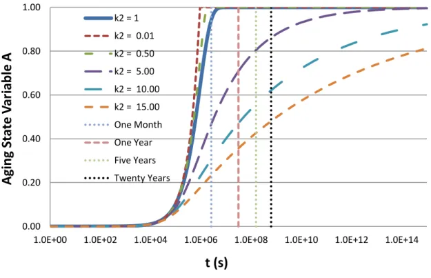
2.4.3 Aging Models for HMA ... 66
2.5 Mechanical Models with Coupled Aging ... 70
3 MATERIALS AND METHODS ... 72
3.1 Investigated Asphalt Mixtures ... 72
3.2 Testing Procedures ... 74
3.2.1 Stiffness Characterization ... 74
Resilient Modulus (RM) ... 74
Complex Modulus (E*) ... 74
3.2.2 Permanent Deformation Characterization ... 75
3.2.3 Fatigue Characterization ... 76
Controlled Crosshead Tension Compression Fatigue Tests ... 76
Controlled Force Indirect Tensile Fatigue Tests ... 77
3.2.4 Experimental Campaign ... 78
4 RESULTS AND DISCUSSION ... 81
4.1 Linear Viscoelastic Characterization and Aging ... 81
4.2 Permanent Deformation Characterization ... 90
4.3 Fatigue Characterization ... 93
4.4 Conventional Characterization Results ... 101
4.5 Mechanical Models with Coupled Aging Results ... 104
4.6 Simulation of Mixture Behavior ... 108
5 CONCLUSIONS AND RECOMMENDATIONS FOR FUTURE WORK ... 110
APPENDIX A - Summary of Results ... 122
1 INTRODUCTION
Asphalt mixture mechanical characterization in Brazil is today primarily based on resilient modulus and indirect tensile strength tests. There is still no national standard for fatigue or permanent deformation mixture characterization. In some specific situations, especially in road concessions to the private industry, controlled force indirect tensile test at room temperature is used for the former, and laboratory traffic simulators or unconfined dynamic creep (flow number) test is used for the latter. Brazil is currently undergoing a national effort to develop its own mechanistic-empirical asphalt pavement design method, based on a national pavement material database and on the performance of test sections monitored throughout the country. A first version of the design guide is planned for 2016.
When it comes to mixture characterization in Brazil, the use of complex modulus is still restricted to academia and research centers. Therefore, it should not be considered in this first phase of the design method, which is being planned in such a way to be systematically updated. For that very reason, it is recognized the importance of leveling the country’s research with international state-of-the-art developments. In this context, the present work deals with the improvement of test and analysis procedures for the characterization of asphalt mixtures considering the dependency of their properties on aging evolution. The research associated with this thesis is focused on aging and on how it relates to mechanical characterization of asphalt mixtures. Stiffness measurements at different aging conditions are used to fit the aging model. Although resistance to permanent deformation is evaluated from an experimental point of view, most of the modeling efforts in this thesis concentrate on fatigue modeling. Therefore, it deals with the coupling of viscoelasticity, viscoplasticity and damage responses to the aging of HMA. More modeling efforts are expended for the fatigue characterization. It is believed that viscoplastic behavior of asphalt materials is affected by aging in such a way that materials become more resistant to the related distress, i.e., permanent deformation. Nevertheless, this work is concerned by the change in the material properties occurring due to aging, that may impact pavements analysis and design.
fatigue characterization, despite extensive literature comments on its influence. Therefore, this work will contemplate the incorporation of aging to the modeling of the mechanical behavior of hot mix asphalt (HMA) during load-induced damage. Although permanent deformation characterization is considered to be a secondary concern in comparison to fatigue when it comes to the consequences of aging, the impacts of aging on HMA resistance to permanent deformation is also presently studied. Stiffness modeling is the input used to calibrate the aging model. Then, it is possible to couple the aging model to viscoplastic and damage models presented in the literature. As previously mentioned, this research is part of a broader project related to the development of the new Brazilian mechanistic-empirical asphalt pavement design method. For this M.Sc. thesis, data for four aging states were available: unaged mixture (Age Zero), aged mixture for 2 days at 85ºC (Age 2, 85ºC), aged mixture for 2 days at 135ºC (Age 2, 135ºC), and aged mixture for 45 days at 85ºC (Age 45, 85ºC). Aging was induced to the loose asphalt mixture, in a procedure adapted from a RILEM protocol, presented in Partl et al. (2012).
Concerning the aging considerations in stiffness characterization of bituminous materials, previous works have presented viscoelastic models which included aging time as a variable (Daniel et al., 1998; Michalica et al., 2008) in addition to loading time (or frequency). However, these models are not conceived to allow easy coupling of aging to other mechanical characteristics of the asphalt mixture, such as viscoplasticity (which deals with intrinsic material properties linked to permanent deformation distress) or damage (which deals with intrinsic material properties linked to fatigue distress). This has motivated the use of the aging phenomenological model proposed by Al-Rub et al. (2013) in the present research. The referred approach couples aging to linear viscoelastic, viscoplastic and damage responses of asphalt mixtures.
Complex modulus results can be used to fit linear viscoelastic models at different aging states. The comparison between the linear viscoelastic parameters obtained at the different aging states allows the identification of the aging model parameters along with the linear viscoelastic parameters' aging sensitivity. With the fitted aging model parameters, viscoplastic model parameters and damage model parameters sensitivity can be estimated comparing experimental results obtained at different aging states, as shown by Al-Rub et al. (2013).
The present document contains aging modeling results obtained by comparing linear viscoelastic models from different aging states. Then, an attempt to couple these models to permanent deformation and to fatigue characterization is made. An aging experimental procedure is also proposed for asphalt mixtures herein as a contribution of the referred research under development.
1.1 Problem Statement
How can pavement analysts model fatigue damage in asphalt mixtures in a more realistic way?
How should asphalt mixture aging be considered when performing laboratory HMA mechanical characterization (stiffness, resistance to permanent deformation and to fatigue)?
Is asphalt mixture resistance to permanent deformation positively affected by aging? What is the impact of aging temperature in the consequences (change in mechanical
properties) of the aging process?
How such considerations change the predicted service life of a typical asphalt mixture within a pavement system?
1.2 Research Objectives
The main objective of this work is to contribute to aging modeling incorporation into hot mix asphalt (HMA) models (stiffness, resistance to permanent deformation and to fatigue). As specific objectives, the following can be listed:
To establish in the Pavement Mechanics Laboratory of Universidade Federal do Ceará a fatigue modeling framework based on solid concepts from continuum damage theory which is still narrowly studied in Brazil;
To explain stiffness changes due to different aging processes based on an aging phenomenological model, and to couple the aging model to a damage model;
To investigate changes on HMA resistance to permanent deformation due to aging; To evaluate the impact of the aging temperature in the HMA mechanical properties; To investigate the impact of aging considerations on the estimated service life of a
typical asphalt mixture.
2 LITERATURE REVIEW
The materials available in nature have the ability to store or to dissipate mechanical energy received through loading when subjected to stress and strain. Equations relating stress and strain (and possibly its derivatives) are known as constitutive equations (or models) and the parameters (or model constants) are usually considered as material properties. For purely elastic materials, it is assumed that all mechanical energy supplied to the system is stored, both for linear and nonlinear elasticity. For the first, stress and strain correlate following a linear proportionality law, represented by the Young's Modulus E, given in stress dimensions, while for the latter, this linear proportionality does not occur. For both cases, stress (σ) depends only on the instantaneous specific deformation, or strain (ε). Consequently, the stress path during loading is always superimposed by the path during unloading (arrows in both senses indicated in Figure 1).
Figure 1 – Generic Stress versus Strain diagram (Babadopulos, 2013)
Some materials, however, do not store nor dissipate entirely the mechanical energy absorbed during loading. In such cases other models may be a better representation than elastic or viscous models. Those are known as viscoelastic models. When viscoelastic materials are subjected to fast loading (high frequencies), they exhibit a behavior close to the one of elastic solids (total storage of mechanical energy). On the other hand, when slow loading is applied (low frequencies), viscoelastic materials exhibit slow deformations, flowing with time, close to viscous fluids behavior (total dissipation of mechanical energy). This is the case of asphaltic materials, which are the object of this thesis.
Usually, associations of springs and dashpots are a good choice for modeling viscoelastic behavior in a first approximation. However, in viscoelastic materials, energy can be dissipated in many ways, such as heat and volumetric damage. These material mechanical responses can either present linear or nonlinear behavior with respect to solicitation (stress or strain). Such nonlinearity can be either reversible or irreversible. If it is irreversible, it can be considered as damage, because it permanently changes the material properties. If it is reversible, it means that it did not change the material properties and it is not desirable to account for it as damage, but as a material intrinsic nonlinearity or possibly as a geometric nonlinearity. In principle, for both cases (recoverable nonlinearity and damage), the phenomenon needs to be taken into account in the constitutive equations in order to maintain a powerful predictive model. In addition, with time and despite the possible inexistence of loading, materials can change their properties. In the literature, this phenomenon is known as aging and in bituminous materials it occurs mostly for two reasons: volatilization of light fractions and oxidation. Some attempts for the consideration of all aforementioned phenomena (linear viscoelasticity, recoverable nonlinearities, damage and aging) are discussed in this Literature Review. The phenomenon of healing (closing of crack openings and consequent recovery of material integrity) is not a subject of the present work although it is widely accepted that it plays an important role in providing extra service life for asphalt pavements.
2.1 Linear Viscoelastic Models
of mathematical functions are extensively used in the literature to represent viscoelastic properties: (i) those based in generic functions (such as power law series or sigmoidal functions), and (ii) those based in mechanical analogs (analogical solution for the mechanical response of an association of springs and dashpots to loading). Despite the fact that good fittings are generally obtained when using generic functions to represent bituminous materials behavior, the results (material constants) are usually difficult to interpret from a physical point of view and not handy to be mathematically and computationally manipulated. For such reasons, the fitting of viscoelastic properties using those functions will not be object of this study. The works by Williams (1964) and by Park et al. (1996), relative to power laws, by Witczak and Fonseca (1996), Christensen et al. (2003) and by Bari and Witczak (2006), relative to sigmoidal functions, are recommended for the reader. On the other hand, models based on mechanical analogs, using an association of springs, dashpots and sometimes stick-slip components, allow a more simple physical interpretation. In the present work, plasticity modeling through mechanical analogs is not evaluated, then stick-slip elements will not be presented. Models using those kind of analogs applied to bituminous materials may be found in Di Benedetto et al. (2007a).
Figure 2 – Linear Viscoelastic Models
(a) Maxwell-Wiechert model (above) (b) Kelvin-Voigt model (below)
For each viscoelastic element (spring-dashpot), a time constant is defined. The variable (given in time dimensions) is known as relaxation time in the Maxwell-Wiechert model, and (also in time dimensions) is known as retardation time in Kelvin-Voigt model. In addition, E∞ is known as the long-term modulus. The elastic compliance of an element Di is defined as the inverse of its elastic constant Ei.
The analytical functions (relating stress and strain) obtained for these models based in linear mechanical analogs are known as Prony (or Dirichlet) series. Prony series is the most common and convenient way to represent the linear viscoelastic behavior of solid continuum media, especially bituminous materials (Soares e Souza, 2003).
For a constant strain ( ), stress decreases with time ( ) (relaxation phenomenon) at a given temperature. For that temperature, the uniaxial tension-compression relaxation modulus ( ) is written as the ratio between the necessary stress and the imposed constant deformation. The Prony series which represents the relaxation modulus for the generalized Maxwell model is indicated in Equation 1.
The parameters , and define a Prony series composed by n elements which represents the linear viscoelastic properties of the studied material.
For the case of a solicitation with constant stress (static creep), strain grows with time (viscoelastic flow). A Prony series for the creep compliance ( ) is analytically obtained for the generalized Voigt model and is represented by Equation 2.
(2)
The parameters , and also define a Prony series composed by n elements which represent the linear viscoelastic properties of the studied material. The set of relaxation times associated to its respective relaxation magnitudes Ei is known as discrete viscoelastic relaxation spectrum. Similarly, the set of retardation times associated to its respective compliance magnitudes Dj is known as discrete viscoelastic retardation spectrum (Ferry, 1980). Those spectra can be generalized when the number of elements tends to infinity. The resulting continuous function relating modulus (or compliance) and time is known as relaxation (or retardation) spectrum. According to Silva et al. (2008), from eight to fifteen viscoelastic elements are necessary in order to have a good fit to experimental data. This depends on the time scale length of available data, generally one order of magnitude in the time domain being covered by one viscoelastic element.
retardation spectra of viscoelastic materials, Prony series is easier to manipulate for the purpose of this work, which includes integration in the time domain.
As complementary information, some models based on parabolic elements can be cited: Huet (Huet, 1963), Huet-Sayegh (Sayegh, 1965) and 2S2P1D (two springs, two parabolic dashpots and one dashpot) (Di Benedetto et al., 2004, 2007b) models. These models represent a gradual evolution from Huet's to 2S2P1D model by the inclusion of other mechanical analogs, which generate new constants to determine. Huet (1963) used only one spring (one constant) and two parabolic dampers (each one with two constants, resulting in five constants). Huet-Sayegh's model used one more spring associated in parallel with the Huet's model (total of six constants). Finally, 2S2P1D introduces, in addition to the past model, a linear damper in series with the Huet's element (total of seven constants). More information about those kinds of models can be found in Pronk (2003, 2006), Woldekidan (2011) and Babadopulos (2013).
Viscoelastic materials present strain response in a given instant depending not only on the stress in that instant but also on all stress history (Christensen, 1982). With the application of the Boltzmann superposition principle (Boltzmann, 1874) to a set of infinitesimal unit step functions applied as solicitation, the so-called convolution integral is obtained, representing the generic linear viscoelastic constitutive model in its integral form. This integral represents linear viscoelastic behavior independently of the chosen mathematical functions to represent the material response (Power laws, Prony series, etc). The convolution integral can be written either representing stress as a function of strain history (Equation 3) or strain as a function of stress history (Equation 4). Strain (ε) and stress (σ) must be continuous and differentiable (smooth) with respect to time, in such a way that both derivatives exist.
; (3)
or
; (4)
linear viscoelasticity is restricted to conditions of small strains, which are satisfied in many theoretical problems, but cannot be assumed in some real cases (Soares e Souza, 2002). Souza (2012) presents a model which considers large strains (inducing nonlinearity) applied to the behavior of asphalt binders.
The relaxation modulus and the creep compliance are fundamental material properties representing the same characteristics of a given material, i.e., linear viscoelastic behavior. Consequently, they are not independent. Therefore, for the experimental characterization of the linear viscoelastic properties of a material, only one of them is necessary. However, differently from purely elastic materials, modulus and compliance are not simply reciprocal quantities (E D ≠ 1). In fact, starting from the convolution integrals, it can be shown in Equations 3 and 4 that one property can be deduced from the other through Equations 5 and 6, i.e., those properties are interconvertible. This kind of procedure by which a property is obtained from the other is known as interconversion.
; (5)
or ; (6)
The aforementioned properties (relaxation modulus and creep compliance) are given in the time domain, being functions of time, so they are said to be transient. Park and Schapery (1999) presented mathematical methods to obtain the relaxation spectra from the retardation spectra and vice-versa.
(7)
Where .
is known as the storage modulus and represents the stored portion of the mechanical energy during harmonic loading. It can be mathematically represented by
Re(E*) (real part of the complex modulus). is known as the loss modulus and represents the dissipated portion of the mechanical energy during harmonic loading. It can also be mathematically represented by Im(E*) (imaginary part of complex modulus). It is to be observed that ω represents the pulsation (or angular frequency), generally expressed in rad/s, and it is directly related to the loading frequency f, in Hz, as .
As the relaxation modulus, the storage and the loss modulus can be represented by analytical equations deduced from exactly the same mechanical analogs used before for the deduction of the Prony series in relaxation (Equation 1). It can be shown that, assuming the generalized Maxwell model for the representation of linear viscoelasticity, the storage ( ) and the loss ( ) moduli are calculated from Equations 8 and 9, respectively.
(8)
(9)
The absolute value (or norm) of the complex modulus ( ) grows with the increase in loading frequency, and decreases with growing temperature. In the literature, most authors refer to this property as the dynamic modulus, although it does not deal with inertial properties. This property, along with the phase angle, describes the behavior of linear viscoelastic materials in the frequency domain. It is to be noted that the model parameters in Equations 8 and 9 (frequency domain) and in Equation 1 (time domain) are the same, in such a way that time and frequency domain properties are interconvertible.
for asphalt binders, but the presence of aggregate particles changes this trend in asphalt mixtures. The temperatures at which those behaviors are observed depend strongly on the analyzed material. In the case of asphalt mixtures, a composite material (thus, heterogeneous), the interlocking provided by the aggregates avoids the occurrence of the phase angle trend approaching 90º at high temperatures. In this case, actually, the phase angle does not present a monotonic trend. Generally, at the zone of low frequencies and high temperatures it grows with loading frequency, while at high frequencies and low temperatures the inverse occurs. This was observed by many authors in the literature (Clyne et al., 2003; Flintsch et al., 2005). The phenomenon can be explained by the fact that the elastic behavior ( ) of the aggregates influences more the material response when the asphalt binder is softer, i.e., at low frequencies and high temperatures (Flintsch et al., 2007). At those conditions, a decrease in frequency leads to a more elastic response, because the contribution of the aggregate particles to the material behavior becomes more important. Consequently, the phase angle decreases.
Generally, the value of the parameters in the Prony series are selected in order to fit linear viscoelastic experimental data. The data can be obtained from experiments conducted in the time domain, such as the relaxation modulus (Equation 1) and the creep compliance (Equation 2), or in the frequency domain, using the storage modulus (Equation 8) and the loss modulus (Equation 9). The fitting procedures are analogous. In this work, storage modulus data are used.
Schapery (1962) introduced the Collocation method for obtaining the parameters of a Prony series, using algebraic linear systems. Only a few experimental points are used in the fitting. The time constants (relaxation or retardation times, depending on the adopted model) are chosen among the experimental data points. The time constants are placed in the same location (collocated) of some of the observed experimental times. The free stiffness constant (known as the long-term modulus) also needs a preestablished value, being typically assumed as the lowest modulus experimentally observed. As mentioned by Sousa et al. (2007), in the case of the relaxation test, for example, this constant assumes the value of the final plateau (when time tends to infinity) of the relaxation modulus curve. For the storage modulus curve, this corresponds to the initial plateau (frequency tends to zero).
obtained experimental result at that collocated point. The simplicity of this method is its main advantage over others to fit Prony series. However, one can only take the collocated points into account when choosing the value of the model parameters. In addition, the same number of elements and experimental collocated points needs to be used, in such a way that only between around 2 and 15 experimental points can be used. The fact that not all experimental points are used, together with the subjectivity about the choice of these points, interferes in the model fitting and, thus, on its predictions. This makes it an obsolete procedure, although it is the basis of other procedures used to fit Prony series. Sometimes, a particular choice of time constants leads to associated stiffness constants with negative values. Such results are not desirable, because the model loses its physical meaning, due to the fact that some of the viscoelastic elements will tend to shorten when tensioned and extend when compressed. This can be avoided changing the choice in the time constants until strictly positive stiffness constants and a good fit are obtained.
In order to take into account all experimental data points, one can elaborate a least squares method. Babadopulos (2013) used Equation 8, which describes the storage modulus using a generalized Maxwell model, and assumed preestablished values for the time constants. One can write the cost function to minimize as
. It can be shown that, when the necessary condition for the
minimization of the cost function is imposed (first derivatives with respect to the stiffness constants equal to zero), the optimum values of the constants are obtained through Equation 10. As in the Collocation method, the value of the long-term stiffness is assumed as the lowest obtained modulus. Equation 10 represents the algebraic linear system whose solution is the set of stiffness constants associated to the preestablished time constants in order to fit storage modulus (frequency domain) experimental results using a linear least squares method. It is capable of considering all M experimental points . The dummy variable (index) represents the lines of the linear system to solve and it varies from 1 to (number of elements in the Prony series).
Silva (2009) presented a linear equation analogous to Equation 10, used for the fitting in the time domain. The great feature of the linear least squares method is to maintain the simplicity of the Collocation method, but taking into account as many experimental points as desired. Besides, the residual square error can be used as an indicator of the goodness of the fit (Babadopulos et al., 2010). As in the Collocation method, the time constants values are still preestablished, which can modify the prediction of the model. However, in the case where all obtained stiffness constants are positive, the prediction of the models obtained from two different choices of time constants is generally similar. Considering that the modulus and the phase angle at a given loading frequency and temperature characterize the linear viscoelastic behavior and not the isolated Prony series constants, it can be said that the results obtained using the linear least squares method are sufficient to model the linear viscoelastic behavior of materials. The time constants need to be chosen in such a way that all stiffness constants are positive. Babadopulos (2013) listed some practical rules in order to obtain them:
One should choose a value near the lowest experimental modulus value (or the highest for the compliance) for the free stiffness constant (or ); Following Schapery's (1962) recommendation, one should place time
constants around one logarithmic decade apart (difference of around one order of magnitude between two consecutive time constants);
It is possible to leave non collocated at most the first and the last logarithmic decades where experimental data is available;
It is recommended to use the maximum number of elements possible which do not return negative stiffness constants;
In case there are negative stiffness constants being obtained, the time constants can be shifted in the logarithmic scale (multiplied by an arbitrary factor) within the experimental results spectrum prior to a new trial;
If there are still negative stiffness constants, the number of elements can be reduced;
(such as power laws) for later fit a Prony series. Park and Kim (2001) and Sousa et al. (2007) are recommended for the reader;
It is desirable to visually analyze the fit obtained, with plots of experimental data and model prediction. Sometimes, very good fits, with
R² near 1, which means that the spectrum of experimental data points are very well predicted by the model, shows unrealistic extrapolations. Still, even with good model fits, it is not recommended to use extrapolations, using only information within the spectrum used for the calibration of the model.
It is to be noted that the linear viscoelastic model is restricted to certain stress and strain levels, which are material dependent. For asphalt mixtures, it is commonly said that the behavior is linear viscoelastic for strains smaller than 150µε (Zhang et al., 2012). Even in this condition, for too many loading repetitions, fatigue damage can evolve. In this case, physical (not geometric) nonlinearity needs to be included in the constitutive models. This is discussed later in this work.
2.1.1 Stiffness Characterization
For the elastic analysis of asphalt pavements, the most used stiffness parameter in Brazilian state-of-practice is the resilient modulus (RM), whereas in North America and Europe, the dynamic modulus is widely used. For analysis involving viscoelasticity, RM is not suitable, and the dynamic modulus must be adopted. Unfortunately, this is still restricted to academia in Brazil. A brief review of these stiffness parameters is presented in this section.
Resilient Modulus (RM): an "elastic" parameter
0.1s loading and 0.9s rest periods, using the lowest force necessary to produce enough deformation for the LVDT measurements. RM is defined as the relation between the deviatoric tensile stress and the "recoverable" extension strain. The definition of "recoverable" strain varies from standard to standard, being a portion of the total strain generated in a loading cycle. The calculation of the RM is made using cycles occurring after some conditioning. Because of the assumption that recoverable strain is used in the calculation of RM, it is considered that only elastic strain is used in the calculation, although from the point of view of the theory of viscoelasticity this is not true (Soares and Souza, 2003; Theisen et al., 2007). During the conditioning cycles, the RM value changes from a cycle to the following cycle more than during the cycles after that conditioning process, because the material is viscoelastic and it flows more in the beginning of the test, before a kind of "steady state" is reached.
The RM test is most commonly conducted in pneumatic testing machines in Brazil. The loading pulse can be modeled by a haversine function, although in pneumatic machines only the load peak and the loading time are controlled by targeting a given cylinder pressure and a given opening time of the solenoid valve. Although vertical and horizontal measurements of the displacement of the samples are most indicated to estimate center point strains in the sample, it is more common to measure only horizontal displacement using two LVDTs mounted touching the surface of the sample.
Complex Modulus (E*)
The complex modulus test consists of applying harmonic compressive loading and obtaining the resulting strains using LVDTs mounted to the sample. Samples of 100mm in diameter by 150mm in height are generally used. Two standards are more frequently used: AASHTO TP 62-03 (2005) and ASTM D 3497-79 (2003). AASHTO TP 62-03 (2005) provisional standard was more recently established as AASHTO T 342 (2011), but consisting in the same procedure. Testing at different temperatures (temperature sweep) and using different loading frequencies (frequency sweep) together with the application of the Time-Temperature (or Frequency-Time-Temperature) Superposition Principle (TTSP) allows the construction of master curves for both the dynamic modulus and the phase angle. The master curves are important tools to characterize viscoelastic materials such as asphalt mixtures (Medeiros, 2006) and some methods to obtain them are presented in the following section. Using the master curves, linear viscoelastic models can be fitted to the experimental data (Lee and Kim, 1998a; Park and Kim, 1998; Daniel and Kim, 2002; Soares and Souza, 2002; Silva, 2009; Babadopulos, 2013), prior to simulations of any kind of loading and the estimation of the corresponding response.
2.1.2 Master Curves Construction
In order to fit linear viscoelastic models to stiffness data obtained with temperature and frequency sweeps, it is necessary to arrange the data in a single smooth curve representing the linear viscoelastic behavior of the material. Such curve is known as the master curve.
Figure 3 – Example of Isotherms for the dynamic modulus
In order to gather the results in a unique curve representing all the data set, two approaches are generally applied. The first one is to eliminate the parameter frequency, representing data in ordered pairs of viscoelastic properties obtained at the same temperature and frequency. Examples of these are the Black space ( ; ) and the Cole & Cole plans ( ). The second approach is the horizontal translation of the isotherms based on the TTSP Principle and this is the most common in the HMA characterization. Materials obeying the TTSP principle are said to be thermoreologically simple, as HMA is typically assumed to be. The TTSP can be understood as the existence of two different sets of temperature and loading frequency that lead to the same value of a linear viscoelastic property. This can be mathematically expressed as in Equation 11.
(11)
Where is the absolute test temperature (in K) and is the adopted reference absolute temperature (in K). The function is usually adopted to have the form
. It is to be observed that, in a logarithmic space, becomes , which means that, indeed, a translation of
, that depends on the test temperature and is known as shift factor, given to the original loading pulsation in a logarithmic scale, leads to the construction of a master curve. The frequency that results from the shift is said to be the reduced frequency. Analogously, the reduced pulsation results from the shift of the physical pulsation. In addition, in the time domain, the application of the TTSP is represented by , where represents the
1.0E+01 1.0E+02 1.0E+03 1.0E+04 1.0E+05
0.1 1 10 100
D
y
n
a
m
ic
M
o
d
u
lu
s
(M
P
a
)
Frequency (Hz)
reduced time and the shift factor is exactly the same as for the shift in the frequency domain.
Three kinds of functions are frequently applied to relate the shift factor to the test temperature. The first one is a polynomial curve fit, the second one is the Arrhenius law, in Equation 12, and the third one is the WLF law (Williams-Landel-Ferry presented in Williams et al., 1955), in Equation 13.
(12)
(13)
In these equations, is the flux activation energy of the material (in kJ/mol.K), is the gas constant ( ), (dimensionless) and (in K) are the coefficients of the WLF law.
Figure 4 – Master Curve examples and shift factors curve fitting comparison using Arrhenius and WLF law
(a) (b)
WLF law was chosen in this research because, for the available data, it provided better curve fits and thus produced smoother master curves. As it can be seen in the example in Figure 4b, fitting for the Arrhenius law is less curved, because of the use of only one curve parameter and, thus, fitting is less accurate for the highest and the lowest temperatures. For the example presented, the square error was more than 9 times lower when using WLF when compared to using the Arrhenius law. The fits were obtained using a Solver to run a least squares method, varying the curve parameters.
2.2 Viscoplasticity
Although fatigue is the main concern of the present research, viscoplastic characteristics of HMA are likely to considerably change with aging, altering HMA resistance to permanent deformation. As this occurs in such a way that HMA resistance increases, modeling efforts on the topic are secondary on this thesis. For the subject of HMA viscoplasticity, the reader is directed to the works by Di Benedetto et al. (2007a), Yun and Kim (2011), Subramanian (2011), Choi et al. (2012) and Choi (2013). At Universidade Federal do Ceará, Nunes (2006) applied a viscoplastic model by Tashman (2003) to asphalt mixtures containing calcinated clays as coarse aggregates, and there is ongoing research by Borges (2014) using the model developed by Choi (2013).
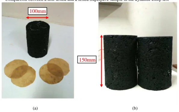
The most used tests for accessing viscoplastic characteristics of HMA are the so-called dynamic creep tests. These tests consist in the repetition of cycles of load and rest periods. Different load functions can be used, such as Heaviside (rectangular shaped) or haversine loading (similar to the pulse used in complex modulus tests). If the Heaviside
1.0E+01 1.0E+02 1.0E+03 1.0E+04 1.0E+05
1.0E-05 1.0E-02 1.0E+01 1.0E+04 1.0E+07
D y n a m ic M o d u lu s (M P a )
Reduced Frequency (Hz)
-10C 4.4C 21.1C 37.8C 54.4C
-6.00 -4.00 -2.00 0.00 2.00 4.00 6.00
260.0 280.0 300.0 320.0 340.0
lo g ( a T ) T (K)
Experimental shift factors
Arrhenius law
WLF law
function is used, the test is equivalent to a creep and recovery test using high stresses (inducing nonlinearity). Different configurations of loading and rest period can be used. Temperature can also be changed and confining pressure can be used at different levels to simulate the confinement of an asphalt layer. All these test parameters change the viscoplastic response of HMA. Thus, full viscoplastic characterization can require 9 test conditions in order to generate a viscoplastic model, adopting models like the ones from Subramanian (2011) or Choi (2013), for example. When testing involves confining pressure, this kind of dynamic creep test is sometimes called triaxial repeated load permanent deformation (TRLPD) test.
Figure 5 – Illustration of HMA behavior under dynamic creep tests (dashed blue line corresponding to the total permanent deformation and continuous red line corresponding to the rate of total permanent deformation
2.3 Viscoelastic Continuum Damage Models
According to Teixeira et al. (2007), the main viscoelastic continuum damage (VECD) models for HMA are based in the work by Schapery (1990a, 1990b), Park et al.
(1996), and Lee and Kim (1998a, 1998b). They define evolution laws for internal state variables through strain energy and the elastic-viscoelastic correspondence principle (Schapery, 1984) to characterize the evolving damage primarily under monotonic loading (Kim and Little, 1990; Park et al., 1996; Daniel and Kim, 2002). This type of damage model, obtained from monotonic testing, is capable of capturing damage dependency on strain (or stress) history and on temperature, which is directly related to fatigue. However, monotonic tests cannot be used to define fatigue failure, because there is no cyclic loading. More recent research efforts (Underwood et al., 2010; Underwood et al., 2012) led to the simplified use of these continuum damage models for cyclic tests, and, thus, for the characterization of fatigue failure under cyclic loading of asphalt materials. This section briefly reviews the origins and the evolution of these models for asphaltic materials.
2.3.1 Thermodynamics of Irreversible Processes as Basics for Damage Modeling
The first works in the domain of continuum damage mechanics were conducted in the late 1950's. According to Lemaitre and Chaboche (1990), Kachanov (1958) was the first
0 20 40 60 80 100 120 0 0.5 1 1.5 2 2.5
0 100 200 300 400
to use a continuum variable to indicate the damaged state of a material, through the definition of effective stress. While Kachanov (1958) developed the analysis scope for brittle materials, Lemaitre and Chaboche (1990) worked in extending the theory to plastic materials, together with many others that intended to apply damage mechanics to their field of knowledge. All those authors highlighted the need to characterize the so-called damage tolerant materials, i.e., materials that in service will be damaged in a such way that the structure does not fail, until a certain point of damage evolution is reached. It is exactly how damage evolves and at which point this would lead to failure that the field of damage mechanics is interested in characterizing. Asphalt pavements are an example of damage tolerant structures that should be characterized following this kind of concept.
The so-called work potential models are damage models derived from Schapery's work potential theory (Schapery, 1990b), whose application to viscoelastic materials, such as asphalt mixtures, is described, for example, in Park et al. (1996) and Park and Schapery (1997). According to Krajcinovic (1989), there are three main general characteristics of continuum damage models: i) the mathematical representation of a damage variable; ii) a particular form for the strain energy density; and iii) an appropriate form for the kinetics law defining the evolution of damage. The three elements used in the particular case of work potential models are briefly described in this section.
According to Schapery (1990b), the mechanical behavior of any material can be expressed in terms of relations between generalized forces ( ) and generalized displacements ( ). The existence of a strain energy density function is assumed in a way that it respects the property represented by Equation 14, which defines the relation between generalized forces and generalized displacements.
(14)
existence of many of them. In this kind of formulation, and are frequently referred to as conjugate pairs or conjugate variables, because of the relationship they keep through the partial derivative of the potential. The ISVs serve to account for the effects of damage and also any other microstructural changes occurring during a thermodynamic process. For an arbitrary infinitesimal process which occurs with changes in and , Equation 15 can be written.
(15)
Equation 15 indicates the contributions of the generalized forces (
)
and of the thermodynamic force (defined as
) to the work in an infinitesimal
process. In order to develop an analyzing procedure for ISV evolution, an ISV law must be specified. Such a law is represented by Equation 16.
(16)
Where is a state function of the ISVs. In that equation, the left hand side can be interpreted as the available force producing changes in microstructure (damage and others), while the right hand side can be interpreted as the required forces to do it. Park and Schapery (1997), for example, presented the analysis of a problem setting the evolution law for one ISV as , or . It is to be observed that curve fitting will be needed to link mechanical properties to the ISVs (like the vs curve explained later).
; (17)
Where is called the pseudo strain and is the reference modulus, which is an arbitrary constant that has the same unit as the relaxation modulus . It should be noticed that if value is set to 1 (unity), the pseudo strain will have the same value as the linear viscoelastic stress, predicted from the convolution integral (Equation 3). So, in linear viscoelastic conditions, the pseudo secant modulus (ratio between and , or ) will be equal to one. However, as the internal microstructure changes (such as the evolving damage), the stress actually required for loading may decrease, so the pseudo secant modulus decrease. In other words, the slope of vs decreases. If the changes in the internal microstructure are the only reason for the pseudo secant modulus to change, is only a function of the ISVs, i.e., and . As the problem with viscoelasticity is being regarded through the elastic-viscoelastic correspondence principle, the stress is the conjugate pair of pseudo strain (see Equation 14), i.e.,
. Respecting that relation,
the work potential is chosen to be the pseudo strain energy density function, represented by Equation 18.
(18)
The following reasoning can lead to the definition of damage evolution laws for viscoelastic materials. Materials have a certain potential to absorb energy, but that energy serves both to deform and to change internal microstructure (in the case studied here, to produce damage). One could take the pseudo strain energy density function (which is a work potential linked to the material's ability to recover from deformed state) as the indication of the absorption of the energy during loading. In this case, the damage rate could be linked to the change in pseudo strain energy, for example through
. The time derivative
is a way to explicitly make the ISV a function of time (rate-dependency). Although that equation could be an option of ISV evolution law, Park et al. (1996) stated that it is to be understood that not only the available force for growth of (denoted by ) but also the resistance against its growth are rate-dependent for most viscoelastic materials. This observation was made regarding micromechanics crack-growth laws for viscoelastic materials available in Schapery (1975) and Schapery (1984). Therefore, as the damage state variable in a global scale should in principle be linked to micromechanical properties, evolution laws similar in form to power-law crack-growth laws for viscoelastic materials should be adopted. Most researchers nowadays use damage evolution laws described as in Equation 19.
(19)
In this equation, is a material-dependent constant directly related to creep or relaxation material properties (i.e., its ability to relax stresses). If denotes the maximum log-log derivative of the relaxation modulus of the material over all time spectrum, the expression is commonly used for displacement controlled tests, while is more frequently used for force controlled tests. According to Park et al. (1996), the choice of the expression is linked to the micromechanical behavior of a crack tip in viscoelastic media, which is described in more details by Schapery (1975). In-depth discussion around it is not an objective of this work. It is to be observed that the chosen expression did not lead to a simple unit for the damage variable ( ). A simple way to look to the damage ISV is as a way to "count" damage, so, can be regarded as a "damage counting".
experimentally presented as a function independent of the applied loading conditions (cyclic vs monotonic loading, amplitude/rate, frequency) and temperature, for a given material. This is why the vs curve is commonly referred to as the damage characteristic curve and treated as a material property (as the complex modulus). Another important contribution is the one by Chehab (2002), where it was shown that the time-temperature superposition for an asphalt mixture is not only valid for the undamaged state, but also for the damage states. It is to be noticed that these are very strong assumptions, but they are also very powerful, allowing faster laboratory damage and fatigue characterization of asphaltic materials, combined with the fact that cyclic tests can be used to obtain both the vs curves and the failure criteria. The tests are shorter because of the use of higher loading amplitudes, which lead to fatigue failure more rapidly, consequently reducing laboratory time. In addition, time-temperature superposition coefficients do not need to be fit for each damage state. Together with those advantages, good agreement between prediction and test results and between prediction and real scale data (FHWA Accelerated Loading Facility) have been obtained (Underwood et al., 2009). With the presented basis of the work potential models, the final general expressions which describe the behavior of asphalt concrete under loading that induces damage can be represented by Equations 20 and 21.
(20)
(21)
Where indicates the strain calculated from the stress history considering the induced damage during loading, and is the reduced time and it indicates the application of the time-temperature superposition principle to the analysis of the problem. For time integration (as in Equations 3 and 4) the variable is used. In order to obtain from experiments, both the material integrity and the damage variable must be calculated for each step in time in the test, obtaining and . While can be directly obtained from its definition for each time step, is obtained from the application of the equation representing the damage evolution law (Equation 19 is the most widely adopted).
should present for a given loading path. Comparison between the actual stiffness and the undamaged one can be used to estimate the damage in the sample. The elastic-viscoelastic correspondence principle allows the calculation of material integrity with a simple method, using the definition of reference modulus (ER) and pseudo strain (εR - linear viscoelastic stress σlve
divided by ER, i.e., εR=σlve/ER). The secant pseudo stiffness (SR) is defined as the ratio between the measured maximum stress (σ) and the correspondent pseudo strain (εR
). The normalized pseudo stiffness (C) is defined as the ratio between the actual SR and the initial secant pseudo stiffness (I), and it accounts for sample-to-sample variation of stiffness. This is represented by Equation 22.
(22)
In other words, a comparison between the actual response (measured stress - σ) and the linear viscoelastic predicted one (pseudo strain - εR
=σlve, assuming ER=1) allows the calculation of C, which can be interpreted as the material integrity and can be directly related to Lemaitre and Chaboche's (1990) traditional damage variable (noted in the authors’ books). According to those authors, defining the concept of effective stress as (where the tilde indicates the measure in a damaged state), the mathematical representation for the damage variable could be chosen as (where is the Young's modulus of the material). The referred authors physically defined this variable as the relative (or corrected) area of cracks and cavities cut by the plane normal to the direction of loading. It is to be observed that, in this case, the loss of cross section area due to damage (microcracks) is assumed to be the reason of the modulus decrease. It is important to observe that the viscoelastic continuum damage models are most easily fit to experimental data using direct tension with constant strain rate tests. This is due to the fact that the convolution integral (Equation 3) is most easily solved in an analytical way, for calculating the pseudo strain. In other words, the convolution integral allows easy calculation of the linear viscoelastic stress
that should be obtained in the case where no damage propagates in the sample.
Some last remarks about Schapery's work potential models need to be made. It is to be observed that, prior to the damage modeling, linear mechanical analogs need to be already obtained after stiffness characterization and that damage put aside, the model reduces to pure linear viscoelasticity. This means that no recoverable nonlinearity linked to loading amplitude dependency of the viscoelastic mechanical response is taken into account by the model. Coutinho et al. (2014) discussed the relevance of considering recoverable nonlinearities and used stress sweep tests to estimate the loading level that divided a recoverable nonlinearity zone from the damage zone. It is important to know that other authors (Di Benedetto et al., 2011; Mangiafico, 2014) used strain sweep tests to characterize amplitude dependency of asphalt mixtures and to estimate the decrease in dynamic modulus due to amplitude dependency in cyclic tests and concluded that this kind of nonlinearity can represent most of the change in mechanical response in some cases. Underwood and Kim (2013) also studied this subject, concluding that asphalt mixtures could exhibit nonlinear viscoelastic behavior. However, they combined nonlinear viscoelasticity to the S-VECD model and concluded that for fatigue simulation, it was not necessary to include nonlinearity considerations in the analysis. Following these results, the S-VECD without considerations of strain dependency of the dynamic modulus is sufficient for fatigue modeling.
them a ready-to-use characterization technique compatible with work potential models is yet available.
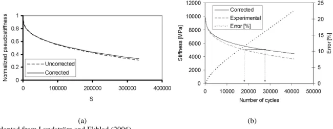
To address the subject of temperature influence on results from fatigue tests obtained using viscoelastic continuum damage models derived from Schapery's work potential theory, one could refer to Lundström and Ekblad (2006). Those authors evaluated 80m diameter by 120mm height HMA samples in controlled strain fatigue tests, while monitoring its surface temperature. The measured temperature indeed increased up to 3ºC at failure for tests at 20ºC and strain amplitude of 500. For that test temperature, dynamic modulus varied 12% for a change in temperature of 1ºC, which justifies the concerns about taking conclusions from tests at those conditions. So, those authors decided to obtain a corrected characteristic curve, by obtaining the reduced time (TTSP) considering the different average temperatures measured at each loading cycle. It was noticed that, although visually the vs curves may appear similar, a simulation of the modulus decrease during the same test conditions could lead to 40% errors in estimating the number of cycles at failure, considering the failure criterion of 50% loss in dynamic modulus. These remarks are illustrated in Figures 6a and 6b.
Figure 6 – (a) C vs S curves obtained from cyclic tests using uncorrected and corrected temperature data at test temperature of 10°C; (b) Simulations of 200 controlled strain test based on corrected and uncorrected
characteristic curves at 10°C.
(a) (b)
Adapted from Lundström and Ekblad (2006)