www.hydrol-earth-syst-sci.net/19/771/2015/ doi:10.5194/hess-19-771-2015
© Author(s) 2015. CC Attribution 3.0 License.
Climate impact on floods: changes in high flows in Sweden in the
past and the future (1911–2100)
B. Arheimer and G. Lindström
Swedish Meteorological and Hydrological Institute, 601 76 Norrköping, Sweden Correspondence to:B. Arheimer ([email protected])
Received: 3 June 2014 – Published in Hydrol. Earth Syst. Sci. Discuss.: 4 July 2014 Revised: 21 December 2014 – Accepted: 7 January 2015 – Published: 4 February 2015
Abstract. There is an ongoing discussion whether floods occur more frequently today than in the past, and whether they will increase in number and magnitude in the future. To explore this issue in Sweden, we merged observed time series for the past century from 69 gauging sites through-out the country (450 000 km2) with high-resolution dynamic model projections of the upcoming century. The results show that the changes in annual maximum daily flows in Swe-den oscillate between dry and wet periods but exhibit no significant trend over the past 100 years. Temperature was found to be the strongest climate driver of changes in river high flows, which are related primarily to snowmelt in Swe-den. Annual daily high flows may decrease by on average
−1 % per decade in the future, mainly due to lower peaks
from snowmelt in the spring (−2 % per decade) as a
re-sult of higher temperatures and a shorter snow season. In contrast, autumn flows may increase by +3 % per decade due to more intense rainfall. This indicates a shift in flood-generating processes in the future, with greater influence of rain-fed floods. Changes in climate may have a more signif-icant impact on some specific rivers than on the average for the whole country. Our results suggest that the temporal pat-tern in future daily high flow in some catchments will shift in time, with spring floods in the northern–central part of Swe-den occurring about 1 month earlier than today. High flows in the southern part of the country may become more fre-quent. Moreover, the current boundary between snow-driven floods in northern–central Sweden and rain-driven floods in the south may move toward higher latitudes due to less snow accumulation in the south and at low altitudes. The findings also indicate a tendency in observations toward the mod-eled projections for timing of daily high flows over the last 25 years. Uncertainties related to both the observed data and the complex model chain of climate impact assessments in hydrology are discussed.
1 Introduction
Numerous severe floods have been reported globally in re-cent years, and there is growing concern that flooding will become more frequent and extreme due to climate change. Generally, a warmer atmosphere can hold more water vapor, in effect leading to a growing potential for intense precipita-tion that can cause floods (Huntington, 2006). Some scien-tists have argued that the observed changes in climate (e.g., increases in precipitation intensity) are already influencing river floods (e.g., Kundzewicz et al., 2007; Bates et al., 2008). However, there are methodological problems associated with detection of changes in floods, and large uncertainties arise when exploring trends in both past and future high flows.
prob-lems by finding more robust methods for analyzing trends and scenario models (see the full review in Hall et al., 2014). Most studies in the literature relate changes in climate to mean annual flow, whereas few concern the impact of such changes on high flows or consider specific drivers. One way to understand changes in flood-generating processes is to analyze seasonality. Some of the main driving pro-cesses (e.g., cyclonic precipitation, convective precipitation, and snowmelt events) are highly seasonal, and thus studying flood occurrence within a year may provide clues regarding flood drivers and changes in those factors (e.g., Parajka et al., 2009; Petrow and Merz, 2009; Kormann et al., 2014).
Hall et al. (2014) argue that future work should exploit, extend, and combine the strengths of both flow record anal-ysis and the scenario approach. The present study concurs with the idea of merging analysis of long time series from the past with dynamic scenario modeling of the future. Cli-mate change detection should be based on good quality data from observation networks of rivers with near-natural condi-tions (e.g., Lindström and Bergström, 2004; Hannah et al., 2010), and time series of more than 50–60 years are recom-mended to account for natural variability (Yue et al., 2012; Chen and Grasby, 2009).
Accordingly, we used time series spanning 100 years (1911–2010) from 69 gauged unregulated rivers to examine recorded changes in flood frequency and magnitude. Mod-eling of the future was performed according to the typical impact modeling chain “emission scenario – global climate model – regional downscaling – bias correction – hydrologi-cal model – flood frequency analysis”, and this was done us-ing the S-HYPE Swedish national hydrological model sys-tem with observed climatology and two 100-year (2000– 2100) climate model projections. An overlapping period of 50 years was applied to check agreement between observed and modeled trends in high flows. The following questions were addressed.
i. What changes have occurred in daily high flows in Swe-den during the last century, and what changes can be expected over the next 100 years?
ii. What climate drivers cause such changes?
iii. How will the flood regime and dominating flood-generating processes change in the future?
2 Data and methods
2.1 Landscape characteristics and high flows observed in the past
Sweden is located in northern Europe and has a surface area of about 450 000 km2. Approximately 65 % of the country is covered by forest, but there are major agricultural areas in the south. Sweden is bordered by mountains to the west and a long coastline to the south and east, and hence the country is drained by a large number of rivers that have their sources in the west and run eastwards to the Baltic Sea and south-west to the North Atlantic. Most of the rivers are regulated, and around 50 % of the electricity in Sweden comes from hydropower. To detect general tendencies in flood change, we aggregated results from analyses of long-term records and scenario modeling to the four regions (Fig. 1) defined by Lindström and Alexandersson (2004). The river basins in these regions show similarities in climate and morphology, but also represent the catchments of the marine basins. Sixty-nine gauges with long records and very little or no upstream regulation in the catchment were chosen from the national water archive to represent the four regions (Fig. 1).
2.2 Model approach to the past and the future
Water discharge and hydrometeorological time series for the past and the future were extracted from the S-HYPE Swedish multi-basin model system (Strömqvist et al., 2012; Arheimer and Lindström, 2013), which covers more than 450 000 km2and produces daily values for hydrological vari-ables in 37 000 catchments from 1961 onwards. This system is based on the process-derived and semi-distributed Hydro-logical Predictions for the Environment (HYPE) code (Lind-ström et al., 2010), and it comprises the Swedish landmass, including transboundary river basins. The first S-HYPE was launched in 2008, but the system is continuously being im-proved and a new version is released every second year. Ob-servations from 400 gauging sites are available for model evaluation of daily water discharge. The S-HYPE version from 2010 was used in the present study.
We forced the S-HYPE model with daily precipitation and temperature data, using national grids of 4 km based on ob-servations and climate model results, respectively. The grid based on daily observations was produced using optimal in-terpolation of data from some 800 meteorological stations, considering variables such as altitude, wind speed and di-rection, and slopes (Johansson, 2002). To study floods, grid-ded values were transformed to each subbasin for the period 1961–2010 to force the S-HYPE model.
Figure 1.Maps showing(a)the four climate regions in Sweden and(b)the locations of the 69 gauges with long-term records from unregu-lated rivers.
the ensemble of 16 climate projections studied by Kjellström et al. (2011), the Hadley projection is among those with the largest future temperature increase in Scandinavia, and the Echam projection represents those with low to medium in-crease. Bosshard et al. (2014) considered all possible selec-tions of two projecselec-tions from this ensemble and noted that the chosen projections spanned a larger uncertainty range than at least 70 % of the other combinations. Both projections simu-lated effects of the A1B emission scenario (Naki´cenovi´c et al., 2000), and the GCM results were dynamically down-scaled to 50 km using the regional climate model (RCM) called RCA3 (Samuelsson et al., 2011). Thereafter, daily surface temperatures (at 2 m) and precipitation were fur-ther downscaled to 4 km, and bias was corrected using the distribution-based scaling method (Yang et al., 2010) with reference data from the 4 km grid-based observations for 1981–2010. Finally, gridded values were transferred to each subbasin for the period 1961–2100 to force the S-HYPE model.
2.3 Quality check and analysis
The capacity of the model to predict annual maximum daily flows was tested at 157 gauging sites without regulation us-ing S-HYPE version 2010. Model deviation for the calibra-tion period and for an independent validacalibra-tion period of the same length was calculated using the forcing grid based on observations. Moreover, simulated trends in the various sim-ulations were compared. Observed and modeled time se-ries for 1961–2010 overlapped, and hence this 50-year pe-riod was used to check agreement between simulations.
Ob-served and modeled results from the 69 river gauges were extracted and compared for different time slots. Simple lin-ear regression was used as a trend test, because a previ-ous study had shown no substantial discrepancy in results obtained by applying different trend tests to Swedish flood data (Lindström and Bergström, 2004). Statistical signifi-cance (P =0.05) was estimated using the formula given by Yevjevich (1972, p. 239).
To explore the spatial variability of climate change, the high-resolution results from the S-HYPE modeling were plotted as maps for two time windows (mean values for 2035–2065 and 2071–2100), showing estimated change for each climate projection. Furthermore, the annual distribution of daily high flows was plotted for the past and future in 15 selected catchments across the country to identify emergent patterns in seasonality.
To quantify temporal changes in annual high flows, we di-vided recorded values for the 69 gauges and modeled data from the 37 000 subbasins by the average value for the refer-ence period (1961–1990) to obtain the relative anomalies at each site. These anomalies were then averaged separately for the country and each region to arrive at a relative change for each domain and each year. Frequency analysis was based on the proportion of gauging sites that exceeded the 10-year flood. The frequency was determined for each year in each region.
coun-try and each region based on site-specific annual anomalies compared to the long-term average for the reference period at each subbasin. Relative changes were considered for aver-age and extreme precipitation, but absolute values were used for temperature (at 2 m).
To distinguish major long-term changes in the flood-generating mechanisms, seasonal changes in magnitude and frequency of high flows were analyzed by separating peaks occurring in March–June and July–February, respectively. In Sweden, spring peaks occurring in March–June along the south-to-north climate gradient are driven mainly by snowmelt, whereas autumn/winter peaks are primarily rain driven. Thus, analyzing each group separately can provide information about any shift in hydrological regime and dom-inant processes that can cause high flows. We also investi-gated variation in timing of daily high flows in specific rivers in 15 selected catchments to assign changes to catchment-specific processes. In this assessment, the last 25 years, which were very mild, were highlighted to illustrate any shift toward the projected future.
Model results presented here were subjected to Gauss fil-tering, with a standard deviation corresponding to a moving average of 10 years, to distinguish between flood-rich and flood-poor periods in the long time series. The trend of the Gauss curves provides a clearer picture of the possible cli-mate trend without the noise from single years. In addition, climate model results for single years should not be regarded as representative of specific years, because such models give long-term projections, not forecasts for individual years.
3 Results
The four hydroclimate regions in Sweden were analyzed both separately and combined using the 69 catchments and the S-HYPE model. However, this showed no clear difference in trends between regions, and therefore all results presented below apply to the entire country.
3.1 Observed annual maximum daily flows during the past
Over the last 100 years, the observed anomalies in annual maximum daily flow were normally within±30 % deviation from the mean of the reference period (Fig. 2). From the 1980s to 2010, the variability in flood frequency was less pronounced. One exception to this was the major flood event in 1995 involving at least a 10-year flood at most of the 69 gauging sites. This was linked to the very high spring flood, especially in the north, where previous maximum discharge records were exceeded by as much as 60 % at some gauges. Spring floods normally corresponded to the annual high flow (cf. the two middle panels in Fig. 2), with a few exceptions, such as the autumn flood in 2000, which affected the central– southern parts of Sweden.
Figure 2.Observed annual high flow (1911–2010) versus the ref-erence period (1961–1990) for the 69 rivers, showing fractions of stations exceeding the 10-year flood each year, the mean devia-tion in the magnitude of annual maximum daily discharge, and the mean deviation in the magnitude of maximum daily discharge dur-ing March–June and July–February. The black line represents a 10-year Gauss filter.
Figure 3.Observed versus predicted annual high flow from the S-HYPE model for(a)the calibration period (1999–2008) and(b)the validation period (1988–1998). MHQ=mean high flow.
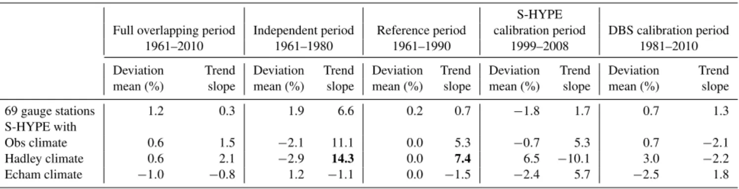
Table 1.Deviation (%) in relation to the mean for the reference period (1961–1990) and trends (slope in percent per decade) for annual anomalies in high flows at the 69 river gauges, using observed discharge from gauges and S-HYPE modeled discharge, the latter with Hadley or Echam forcing from observed climate and climate projections. Bold numbers indicate a significance level ofP=0.05 (Yevjevich, 1972).
S-HYPE
Full overlapping period Independent period Reference period calibration period DBS calibration period 1961–2010 1961–1980 1961–1990 1999–2008 1981–2010
Deviation Trend Deviation Trend Deviation Trend Deviation Trend Deviation Trend mean (%) slope mean (%) slope mean (%) slope mean (%) slope mean (%) slope
69 gauge stations 1.2 0.3 1.9 6.6 0.2 0.7 −1.8 1.7 0.7 1.3 S-HYPE with
Obs climate 0.6 1.5 −2.1 11.1 0.0 5.3 −0.7 5.3 0.7 −2.1 Hadley climate 0.6 2.1 −2.9 14.3 0.0 7.4 6.5 −10.1 3.0 −2.2 Echam climate −1.0 −0.8 1.2 −1.1 0.0 −1.5 −2.4 5.7 −2.5 1.8
3.2 Model performance and comparison of trends in simulations
In the S-HYPE model (version 2010), the median absolute error was 15 % for annual maximum daily flows at 157 gauging sites for both the calibration and validation peri-ods (Fig. 3). Median underestimation was −0.7 % for cali-bration but−3.5 % for validation. The major outliers could be related to some missing lakes in this version of the S-HYPE model, as the model then overestimated high flows because the dampening effect of lakes was missing in the model setup.
Comparison of S-HYPE simulations using different forc-ing data revealed no statistically significant trends in ob-served or modeled high flows for the entire 50-year over-lapping period (Table 1), although there was a small devi-ation between that period and the reference period, which was only 20 years shorter. Accordingly, the trend test de-tected no significant trends in shorter periods, except for the Hadley forcing, which showed statistically significant trends during the independent period and the reference period. In general, climate projections are not necessarily in phase with observed climate fluctuations, which was the case with the projections used in our study. This was also apparent for the longer time period of 50 years, for which the Echam forcing showed an opposite sign of slope compared to forcing with either Hadley or observed climate data.
The slope of the modeled time series using observed cli-mate data was generally larger than the slopes of observed trends. This suggests that the S-HYPE model overestimates the sensitivity to changes in forcing data, or that there are compensating processes not included in the S-HYPE model (e.g., changes in land use, vegetation, or abstractions). The difference in slope may also be an artifact of bias in pre-cipitation data, as discussed by Lindström and Alexanders-son (2004) and Hellström and Lindström (2008). In four of the five time slices we examined, the S-HYPE model forced with observed climate data exhibited the same sign of slope as observed time series of river flow. Again, it should be
noted that none of these trend slopes was statistically sig-nificant (Table 1).
3.3 Future climate projections for Sweden
Figure 4 shows the large differences we obtained in spa-tial patterns of precipitation and temperature across Sweden when forcing S-HYPE with the two future projections. The results for the reference period (1981–2010) were similar for the two climate projections (Hadley and Echam), because precipitation and temperature were scaled against the same 4 km grid based on observations. However, considering fu-ture climate change, results provided by climate models dif-fer greatly and can be conflicting, particularly regarding local conditions.
According to both projections in our study, the mean tem-perature will increase by 3–5◦ in different parts of Swe-den in the future. The Hadley model indicated a more rapid increase compared to the Echam model. The two models projected that average precipitation will increase by 100– 400 mm yr−1 depending on the geographical location, and the Hadley model indicated a faster and more marked in-crease.
Figure 4.Spatial patterns of climate change impact across Sweden obtained using two downscaled and bias-corrected climate projec-tions in S-HYPE. Mean values for the mid-century (2035–2065) and the end of century (2071–2100) are compared with the mean for a reference period (1981–2010). Red indicates warmer/drier, and blue represents colder/wetter. Results are not shown for highly reg-ulated rivers (yellow).
There was ±50 % spatial variation in the future changes
in mean high flow and the magnitude of the 10-year flood (Fig. 4), whereas, for most of the country, such divergence was only 15 %. The estimated levels were highest for the northern part of the mountain range and southwestern Swe-den. The 10-year flood flows were lower for the mountains of Jämtland County, which is one of the areas with the most rich snowfall. There is a large spread in the results for the two projections; hence, the findings regarding high flows on the local scale should be interpreted with caution. The Hadley forcing led to larger changes for the whole country, whereas Echam forcing indicated smaller changes compared to the reference period.
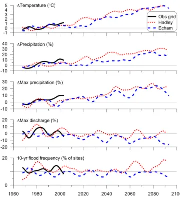
Figure 5. Modeled deviation (%) in annual regional estimates (1961–2100) versus the reference period (1961–1990) using S-HYPE for annual mean temperature and precipitation, maximum daily precipitation, annual daily high flow, and number of gauges exceeding the 10-year flood. A 10-year Gauss filter was used to fil-ter annual results. Modeling was done with forcing data based on observations (Obs grid; solid lines) or on climate models (Hadley and Echam; dotted and dashed lines).
Our findings confirm that assessments of future climate change can differ markedly depending on the climate model that is applied, even if the same emission scenario is used. The two projections in our study were far from covering the full range of uncertainty, although a closer analysis shows that they did include most of the range of the ensemble of 16 climate projections used before, especially at the higher end of the extremes. The corresponding river flows calcu-lated with S-HYPE were within the 25–75 % range of the larger ensemble when using the HBV model (Bergström et al., 2012).
3.4 High flow in the future and climate drivers
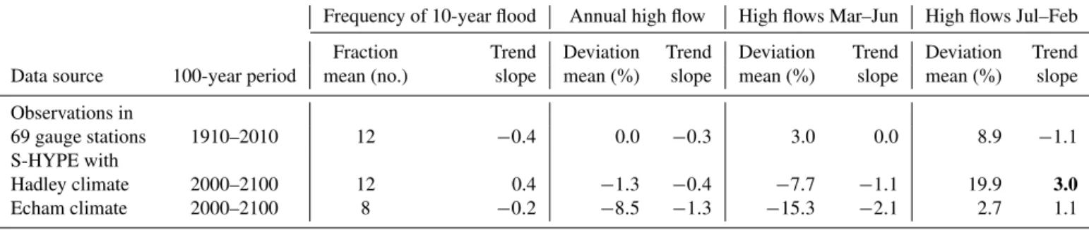
Table 2.Summary of analysis of daily high flows in observed time series representing 100 years in the past and a modeled time series for 100 years in the future. Deviation ( %) in relation to the mean of the reference period (1961–1990) and trends (slope as percent per decade) are given for annual high flows, frequency of 10-year flood, and spring and autumn flood. Bold numbers indicate a significance level of P =0.05(Yevjevich, 1972).
Frequency of 10-year flood Annual high flow High flows Mar–Jun High flows Jul–Feb
Fraction Trend Deviation Trend Deviation Trend Deviation Trend Data source 100-year period mean (no.) slope mean (%) slope mean (%) slope mean (%) slope
Observations in
69 gauge stations 1910–2010 12 −0.4 0.0 −0.3 3.0 0.0 8.9 −1.1
S-HYPE with
Hadley climate 2000–2100 12 0.4 −1.3 −0.4 −7.7 −1.1 19.9 3.0
Echam climate 2000–2100 8 −0.2 −8.5 −1.3 −15.3 −2.1 2.7 1.1
not reflected in the river flow. It should also be noted that the temperature signal during the past 50 years in Fig. 5 is not representative of the twentieth century as a whole (Lind-ström and Alexandersson, 2004).
Considering annual maximum daily flow in Fig. 5 reveals no trend over the past 50 years and a decreasing trend in the future. This can be explained by elevated temperature lead-ing to lower sprlead-ing peaks from snowmelt, caused by a shorter snow period and higher evapotranspiration. The results did not show any clear trend in 10-year flood frequency. Thus, it seems that in Sweden, temperature is stronger than precipi-tation as a climate driver of river high flow, which illustrates that high flows are mainly related to snowmelt in this coun-try.
3.5 Changes in the flood regime
The most substantial effect of changes in floods in Sweden was found when comparing the results of separate analyses of annual maximum daily flows occurring in the spring and in the rest of the year (mainly autumn). Figure 6 shows a significant decrease in magnitude of spring floods and a sig-nificant increase in autumn floods. For spring floods, using observed forcing data resulted in a weak trend, whereas the trend obtained using climate projections indicates a 10–20 % reduction by the end of the century compared to the 1970s.
For autumn floods, the trend was in the opposite direction, with 10–20 % higher magnitudes by the end of the century. However, it should be noted that autumn floods are generally only about half as high as spring floods in Sweden, except in the south, where the autumn and winter flows are normally larger. This also explains why this change in flow regime was not detected when focusing solely on annual maximum val-ues for the whole country, which are dominated by the spring peak caused by snowmelt. There was a notable increase in the observed autumn peaks over the last 50 years, whereas the climate assessment with Hadley forcing revealed the largest increase in trend in the future. These results indicate an on-going shift in flow regime, which can be attributed to flow-generating processes; by comparison, there will be less
im-Figure 6.Modeled annual maximum daily flows during spring (top) and autumn/winter (bottom) for the period 1961–2100. Deviation (%) in magnitude versus reference period (1961–1990). The lines represent a 10-year Gauss filter for S-HYPE modeling using a forc-ing grid based on observations (Obs grid) or climate projections (Hadley and Echam).
pact from floods generated by snowmelt in the spring and more frequent floods caused by intensive rainfall during the rest of the year.
3.6 Combining results to detect long-term changes in high flows
Assessing the past 100 years, we found no significant trends and only very small mean deviation in maximum daily flows (Table 2). The mean deviation for the autumn floods versus the reference period at the 69 river gauges was 9 %, which means that the reference period was not representative of au-tumn floods, as can also be seen in Fig. 2. In contrast to the results for the last 50 years (Fig. 6), we found a negative trend in the autumn high flows for the last 100 years, although this was not statistically significant according to the trend test.
Figure 7.Merged time series of deviations (%) versus the mean for the reference period shown for actual observations (1910–2010) and modeling results (2010–2100) for past and future annual maximum high flows in Sweden. The lines represent a 10-year Gauss filter for observations (Obs) and S-HYPE forced with climate projections (Hadley and Echam).
Echam forcing indicated the largest negative trend, entail-ing on average a more than−2 % reduction in spring peaks each decade. Conversely, there were positive trends in future autumn peaks, especially when using Hadley forcing, which resulted in a +3 % increase per decade. Both these trends for the future were significant atP =0.05, which confirmed the visual inspection of changes in flow regime in the Gauss curves (Fig. 7).
Figure 7 shows that there have been large long-term climate-induced oscillations in maximum daily flows during the last 100 years, which are expected to continue over the next 100 years. Furthermore, the oscillations in flood fre-quency were larger in past observations than in the future projections, although this might represent an artifact of the grid size used in the climate projections, which could have underestimated local extremes. Future long-term trends were consistent between climate projections, but each trend was statistically significant in only one projection (cf. Table 2).
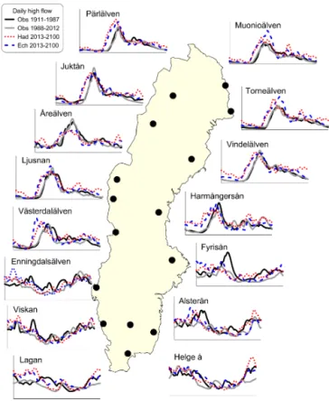
Assessment of the seasonal cycle of high flow distribu-tion in selected catchments indicated a temporal shift in maximum daily flows between the past, present, and future (Fig. 8). The last 25 years (present) have been warm and wet, and have shown a tendency toward the results of the climate projections. Note that the diagrams in Fig. 8 represent time periods of different lengths and show absolute values instead of changes, and hence are not directly comparable but merely illustrate temporal changes during an average year. For the
Figure 8.Annual distribution of daily high flow (Jan–Dec) in se-lected catchments across Sweden obtained using a 1-month Gauss filter for observed and projected time series. Note: magnitudes of observed and projected values are not comparable; only the timing of high flows should be compared. Solid lines represent observa-tions (Obs) for different time periods. Dotted and dashed lines rep-resent S-HYPE modeling with forcing data from the Hadley (Had) and Echam (Ech) climate models, respectively.
future, the results suggest that daily high flows occur about 1 month earlier during the spring in the northern–central part of Sweden and become more frequent in the south, proba-bly due to less snow accumulation in the south and at low altitudes.
4 Discussion
4.1 Changes in high flows in Sweden
This study revealed that a pronounced shift in magnitudes of high flows induced by climate change has not yet been recorded nor is it expected in Sweden. However, our in-vestigation focused on rivers, not on the small-scale flood-ing caused by changes in intense local precipitation, which may have a greater impact in the future (e.g., in urban ar-eas) (Arnbjerg-Nielsen et al., 2013; Olsson and Foster, 2014). We found a small, albeit not statistically significant, nega-tive trend in river high flow, indicating a 0.4 % decrease in 10-year flood frequency each decade. This confirms previous findings reported by Wilson et al. (2010) showing a decrease in peak flow events in long time series from Sweden, Finland, and parts of Denmark, but an increase in series from western Norway and Denmark. However, the changes we detected by using future climate projections in Sweden were statistically significant (P =0.05) and, in some cases, of greater magni-tude. It seems that annual daily maximum high flows may decrease by−1 % per decade in the future, whereas autumn flows may increase by+3 %, but the trends are far from lin-ear. Assessing the maximum deviation versus the reference period shows that 1961–1990 cannot be used as a reference period in the future. Most design variables for infrastructure in Sweden are based on this period, and thus they must be recalculated using a new reference period to adapt them to climate change. Unfortunately, considering the past century, it also appears that 1961–1990 was not particularly repre-sentative of natural variability, especially regarding autumn floods.
Merging Gauss curves using both 100 years of observa-tions and 100 years of climate projecobserva-tions clearly visualized the relative changes in and influence of long-term oscillations (Fig. 7). This combined analytical approach using both actual observations and model results simultaneously provides a broader understanding of natural versus accelerated changes in long time series. Applying shorter timescales to observed climate data gave a very different picture. For instance, when we used the 1960s as the starting point for a 50-year analy-sis (Figs. 5 and 6), it seemed that the trend toward increased autumn floods was already very strong at that time, but this trend disappeared when we used 100 years of observations (cf. Table 2 and Fig. 7). This demonstrates that a period of 50 years is insufficient for detecting trends in the Swedish climate. Lindström and Bergström (2004) found that trend detection is very sensitive to starting and ending years, which agrees with findings from other climate regions (e.g., Han-naford et al., 2013; Yue et al., 2012; Chen and Grasby, 2009). In contrast to the trend analysis, our evaluation of an-nual dynamics and specific catchments revealed more rad-ical changes in high flows. The earlier spring floods in the northern–central part of Sweden, more frequent high flows in the south, and even disappearing spring peaks (Fig. 8), could
be attributed to less snow accumulation in the south and at low altitudes. Similar findings have been made in Austria, where runoff trends could also be linked to altitude within catchments and attributed to changes in various processes dominating at different elevations (Kormann et al., 2014).
Spatial patterns can be noisy and make it difficult to detect overall trends due to local events. We used 69 gauging sites in our study and considered the mean of relative deviation (not absolute values) to be representative of the country. Our frequency analysis also illustrated the spatial extent of spe-cific high flow events. Originally, four hydroclimate regions were included in the evaluation (Fig. 1), but the results con-cerning observed changes differed very little between those regions, which were therefore considered to be too small to represent climate change. However, the projections of future climate differed markedly between the north and the south-ernmost regions (Figs. 4 and 8); for example, the positive trend in autumn flows with Hadley forcing was noted mainly in the north. Trend detection was based solely on spatially aggregated results for the entire domain, because we con-sidered the discrepancies in the projections on a local or re-gional level to be too large to allow high-resolution analysis. Nevertheless, the observed high flow during the last 25 years did show a slight tendency toward the temporal changes that were suggested by the projections for individual catchments (Fig. 8). In addition, separation between rain-fed and snow-generated high flows could have been another basis for re-gional analysis. We therefore suggest a more thorough anal-ysis for clustering catchments with similar behavior in future studies of regional changes within Sweden.
Results regarding the impact of climate change on fre-quency and intensity of floods in northern European coun-tries are also available in the literature. Dankers and Feyen (2008) and Hirabayashi et al. (2008) indicated a de-crease in water flow, whereas Lehner et al. (2006) suggested an increase, and Arheimer et al. (2012) projected very little overall change in water discharge to the Baltic Sea. Discrep-ancies between conclusions regarding the future can arise due to uncertainties in GCMs, downscaling methods, or hy-drological models (e.g., Bosshard et al., 2013; Donnelly et al., 2014; Hall et al., 2014).
4.2 Methodological uncertainties
rivers at the gauges are considered to be rather stable, but a recent updating of a rating curve, after construction work at the gauging site, included changing the estimated water flow by approximately 30 %. When rating curves are updated, the historical flow is also reconstructed. Nonetheless, this can be a major source of error in all analyses using observations of river flow. Extreme high flows are more uncertain than nor-mal conditions, because in such cases the flow can be outside the calibrated range of the rating curve, and the flowing water may take new paths that bypass the gauging station. In Swe-den, ice jam is another common monitoring problem, and hence observed time series are corrected for such blockage and reconstructed annually. These corrections may influence estimates of spring peaks in some of the northern rivers and represent another source of uncertainty.
It is even more difficult to monitor and model precipita-tion, because observations are influenced by changes in veg-etation, wind, snowfall/rainfall, and monitoring equipment. Furthermore, the monitoring technique employed at the be-ginning of last century probably underestimated precipitation (Lindström and Alexandersson, 2004). Experience has also shown that using the 4 km precipitation grid for operational hydrology, as done in our study, underestimates precipitation in the mountains of Sweden by some 10–20 %. Accordingly, use of this grid as a source of observed climate data will ob-viously affect hydrological model results. Our validation of high flows in S-HYPE indicated median absolute errors of 15 and−3.5 % underestimation in unregulated rivers (Fig. 3). Also, Bergstrand et al. (2014) have reported that, after updat-ing the S-HYPE model with gauged flow for national statis-tics and design variables, the mean high flows were underes-timated by 5 % at the 400 gauging stations, including those in regulated rivers. Clearly, the underestimation of high flow is affected by the underestimated precipitation.
Major uncertainties associated with estimating future floods are related to the effects and interactions of the fol-lowing components in the model chain (e.g., Bosshard et al., 2013): (1) climate model projections; (2) downscaling/bias correction techniques; and (3) hydrological model uncertain-ties in the region studied.
4.2.1 Climate models
The discrepancy we found between our climate model pro-jections indicates pronounced uncertainty of the local results, and trends in climate signals were often in opposite direc-tions in the projecdirec-tions. It is well known that precipitation patterns in climate models differ considerably for different parts of Europe (e.g., van Ulden and van Oldenborgh, 2006), and this variability is further increased when extreme events are simulated by GCMs and RCMs (e.g., Blöschl et al., 2007). Hence, the calculations performed are highly uncer-tain, and the findings concerning this part of the world should be approached with caution. Therefore, we limited our anal-ysis to aggregated results concerning changes in floods in
Sweden. It is normally recommended that decisions and im-pact modeling be based on the ensemble mean from many different climate projections (e.g., Bergström et al., 2012), but it is not known how much this will actually reduce the overall uncertainties. Ensemble runs correspond to a sensi-tivity analysis (intercomparison of models) and not to uncer-tainty estimation in the statistical sense. Ensembles can also be biased by using many different versions of a particular model, and the GCMs/RCMs often include similar descrip-tions of the physics. In addition, some processes are not well represented in any climate model.
4.2.2 Downscaling and bias correction
Statistical downscaling and bias correction techniques in-volve empirical correction of simulated climate variables (e.g., precipitation and temperature) by fitting simulated means and quantiles to the available observations and ap-plying the same correction to future simulations (e.g., Yang et al., 2010). Consequently, it is assumed that the observed biases in the mean and variability of those climate param-eters are systematic and will be the same in the future, but it remains to be determined whether the climate model er-rors are static over time (Maraun et al., 2010). Use of bias correction methods leads to a better fit of the hydrologi-cal model output, narrower variability bounds, and improved observed runoff regimes compared to uncorrected climate model data (Bosshard, 2011; Teutschbein and Seibert, 2012). Nevertheless, bias correction can also introduce inconsis-tency between temperature and precipitation, which strongly affects simulation of snow variables (Dahné et al., 2013) and thereby also influences predictions of future floods. Further-more, bias correction is very sensitive to the reference data set applied, and thus conclusions regarding the hydrologi-cal impact of climate change may vary considerably even if all other aspects are kept constant (Donnelly et al., 2013). Therefore, Donnelly et al. (2014) have urged that, in addition to uncertainties in the climate model and scenario, uncertain-ties in the bias correction methodology and the impact model should be taken into account in studies concerning the impact of climate change.
4.2.3 Uncertainties in hydrological models of the studied region
is that it focuses on timing, and its use in optimization can thus underestimate the magnitude of high flow if the timing is not perfect.
The S-HYPE model is also assumed to be valid for un-gauged basins, as has been confirmed by values from blind tests for independent gauging stations comparable to those calibrated for groups of similar catchments (Arheimer and Lindström, 2013). S-HYPE captures hydroclimatic variabil-ity across Sweden, even though the gradients in temperature and precipitation in this country are larger than the estimated change in climate projections. However, variables that are sensitive to temperature (e.g., evapotranspiration) should be validated, in particular to ascertain whether their parameters are realistic for a changing climate. Use of several impact models is also recommended. For instance, Stahl et al. (2012) found that the mean of an ensemble of eight global hydro-logical models of Europe provided the best representation of trends in the observations.
The present scenarios consider changes in atmospheric emissions and concentrations of climate gases. However, in the future, additional changes may well occur in other drivers of the hydrological regime, such as land use and vegetation, or construction work in river channels (Merz et al., 2012), which can also have a large impact on flood generation (e.g., Hall et al., 2014) and add uncertainties to predictions regard-ing flood frequency and magnitude. As described elsewhere (Arheimer and Lindström, 2014), we recently reconstructed the total impact of Swedish hydropower on the river water regime, which showed that spring peaks have decreased by 15 % on a national scale. Hydropower in this country was es-tablished mainly from 1910 to 1970, and this anthropogenic alteration of the water resources has had a larger impact on river high flow than could be expected from climate change.
4.3 Gauss filtering
Statistical trend analyses were performed using discrete val-ues of annual high flows, whereas visual inspections were conducted using a Gauss filter with a standard deviation cor-responding to a moving average of 10 years. Gauss filtering dampens the effect of individual years and facilitates visual discrimination between the trends and oscillations. The filter does not remove all noise, and some oscillations also remain in a random data set. However, a Gauss filter does not intro-duce any new oscillations. This is exemplified by the differ-ence between periods in Fig. 2, which is real and not an arti-fact introduced by the filtering. For instance, the 1970s were dry in practically all of Sweden, whereas the 1920s, 1980s, and 1990s were mostly wet and had more frequent high au-tumn flows. The same periods stand out in other Nordic coun-tries as well. The Gauss filter does not introduce any new trends, as with the ones shown in Fig. 5, since it only aver-ages the signal over time. Hence, the filter is used merely to smooth the signal and compute decadal averages without the disadvantages of an ordinary running average. The Gauss is
a low-pass filter that removes most of the interannual varia-tion, and thus makes it easier to discern changes with a longer timescale (e.g., decades). Interestingly, it seems that the same pattern of more persistent periods of drier and wetter years that has occurred in the past (and is not introduced as an ar-tifact by filtering) is preserved in the climate projections for the future. When making such projections, it is very impor-tant not to analyze specific years, because climate models do not yet offer such predictability, but can only identify general trends and fluctuations that are not necessarily in phase with the observed climate. Therefore, rather than presenting spe-cific years from climate impact modeling, we chose to show only the general tendencies that are illustrated more clearly by Gauss filtering.
5 Conclusions
The present results indicate that there will be some shifts in flood-generating processes in Sweden in the future, and rain-generated floods will have a more marked effect. It is also plausible that there will be a greater climate impact on spe-cific rivers than on the average for the entire country. Un-certainties and simultaneous changes from drivers other than climate must also be accounted for, although our findings do show the following results.
– Changes in annual maximum daily flows in Sweden os-cillate between clusters of years in relation to observed variability in weather, but no significant trend can be discerned over the past 100 years. We found a small tendency toward a decrease in high flows considering both magnitude and 10-year flood frequency, but these results were not statistically significant.
– Temperature is the strongest driver of river high flows, because these events are related to snowmelt in most of Sweden. It is possible that the annual daily maximum flows will decrease in the future, mainly due to lower snowmelt peaks in spring as the result of earlier spring flood. In contrast, more intense rainfall and less snow accumulation may lead to increased autumn and winter flows.
– The temporal pattern of future daily high flows may shift in time and spring floods may occur approximately 1 month earlier in the northern–central part of Sweden and more frequent high flows in the south due to less snow accumulation in the south and at low altitudes. Observations from the last 25 years have already shown a tendency toward this projected change.
Acknowledgements. This study was performed at the SMHI Hydrological Research Unit, where much work is done jointly to take advantage of previous studies and several projects conducted in parallel by the group. Hence, input from individuals other than the authors was essential for the background material and, in par-ticular, we acknowledge the work performed by Johan Strömqvist and Thomas Bosshard for future climate change projections. Funding was provided by Swedish research councils: analysis of recorded flows was done with grants from HUVA/Elforsk, and assessments using model scenarios were funded by projects Hydroimpacts2.0 (Formas) and CLEO (Swedish EPA). Our study will contribute to the Panta Rhei IAHS Scientific Decade initiative concerning changes in hydrology and society, and its working group on floods. S-HYPE results and gauged time series, as well as tools for model uncertainty checks and maps of climate scenario estimates, are available for inspection and free downloading at http://vattenwebb.smhi.se/. Finally, the authors thank Juraj Parajka, an anonymous reviewer, and the Editor Stacey Archfield for valuable comments on the manuscript.
Edited by: S. Archfield
References
Arheimer, B. and Lindström, G.: Implementing the EU Water Framework Directive in Sweden, in: Runoff Predictions in Un-gauged Basins – Synthesis across Processes, Places and Scales, edited by: Bloeschl, G., Sivapalan, M., Wagener, T., Viglione, A., and Savenije, H., Cambridge University Press, Cambridge, UK, 353–359, 2013.
Arheimer, B. and Lindström, G.: Electricity vs Ecosystems – un-derstanding and predicting hydropower impact on Swedish river flow. Evolving Water Resources Systems: Understanding, Pre-dicting and Managing Water–Society Interactions, Proceedings of ICWRS2014, Bologna, Italy, 4–6 June 2014, IAHS Publ. No. 364, 2014.
Arheimer, B., Dahné J., and Donnelly, C.: Climate change impact on riverine nutrient load and land-based remedial measures of the Baltic Sea Action Plan, Ambio, 41, 600–612, 2012.
Arnbjerg-Nielsen, K., Willems, P., Olsson, J., Beecham, S., Pathi-rana, A., Bülow Gregersen, I., Madsen, H., and Nguyen, V. T. V.: Impacts of climate change on rainfall extremes and ur-ban drainage systems: a review, Water Sci. Technol., 68, 16–28, doi:10.2166/wst.2013.251, 2013.
Bates, B. C., Kundzewicz, Z. W., Wu, S., Palutikof, J. (Eds.): Cli-mate Change and Water, Technical Paper of the Intergovernmen-tal Panel on Climate Change, IPCC Secretariat, Geneva, 210 pp., 2008.
Bergstrand, M., Asp, S., and Lindström, G.: Nationwide hy-drological statistics for Sweden with high resolution using the hydrological model S-HYPE, Hydrol. Res., 45, 349–356, doi:10.2166/nh.2013.010, 2014.
Bergström, S., Andréasson, J., and Graham L. P.: Climate adapta-tion of the Swedish guidelines for design floods for dams, 24th ICOLD Congress, Kyoto, Japan, 6–8 June 2012, Q94, 2012. Blöschl, G., Ardoin-Bardin, S., Bonell, M., Dorninger, M.,
Goodrich, D., Gutknecht, D., Matamoros, D., Merz, B., Shand, P., and Szolgay, J.: At what scales do climate variability and land
cover change impact on flooding and low flows?, Hydrol. Pro-cess., 21, 1241–1247, doi:10.1002/hyp.6669, 2007.
Bosshard, T. and Olsson, J.: Comparison of the two climate projec-tions in CLEO to a larger ensemble, CLEO report, 20 pp., avail-able at: http://www.cleoresearch.se/publications/cleoreports(last access: 30 January 2015), 2014.
Bosshard, T., Kotlarski, S., Ewen, T., and Schär, C.: Spectral rep-resentation of the annual cycle in the climate change signal, Hy-drol. Earth Syst. Sci., 15, 2777–2788, doi:10.5194/hess-15-2777-2011, 2011.
Bosshard, T., Carambia, M., Goergen, K., Kotlarski, S. Krahe, P., Zappa, M., and Schar, C.: Quantifying uncertainty sources in an ensemble of hydrological climate-impact projections, Water Re-sour. Res., 49, 1523–1536, doi:10.1029/2011WR011533, 2013. Chen, Z. and Grasby, S. E.: Impact of decadal and century-scale
os-cillations on hydroclimate trend analyses, J. Hydrol., 365, 122– 133, doi:10.1016/j.jhydrol.2008.11.031, 2009.
Collins, M., Booth, B. B. B., Harris, G. R., Murphy, J. M., Sex-ton, D. M. H., and Webb, M. J.: Towards quantifying uncer-tainty in transient climate change, Clim. Dynam., 27, 127–147, doi:10.1007/s00382-006-0121-0, 2006.
Dahné, J., Donnelly, C., and Olsson, J.: Post-processing of climate projections for hydrological impact studies: how well is the ref-erence state preserved? IAHS Publ. no. 359, 2013.
Dankers, R. and Feyen, L.: Climate change impact on flood hazard in Europe: An assessment based on high-resolution climate simulations, J. Geophys. Res.-Atmos., 113, D19105, doi:10.1029/2007JD009719, 2008.
Donnelly, C., Arheimer, B., Bosshard, T., and Pechlivanidis, I.: Un-certainties beyond ensembles and parameters – experiences of impact assessments using the HYPE model at various scales, Proceedings of the International Conference on Climate Change Effects, Potsdam, Germany, 27–30 May, 2013.
Donnelly, C., Yang, W., and Dahné, J.: River discharge to the Baltic Sea in a future climate, Clim. Change, 122, 157–170, doi:10.1007/s10584-013-0941-y, 2014.
Hall, J., Arheimer, B., Borga, M., Brázdil, R., Claps, P., Kiss, A., Kjeldsen, T. R., Kriauˇci¯unien˙e, J., Kundzewicz, Z. W., Lang, M., Llasat, M. C., Macdonald, N., McIntyre, N., Mediero, L., Merz, B., Merz, R., Molnar, P., Montanari, A., Neuhold, C., Parajka, J., Perdigão, R. A. P., Plavcová, L., Rogger, M., Sali-nas, J. L., Sauquet, E., Schär, C., Szolgay, J., Viglione, A., and Blöschl, G.: Understanding flood regime changes in Europe: a state-of-the-art assessment, Hydrol. Earth Syst. Sci., 18, 2735– 2772, doi:10.5194/hess-18-2735-2014, 2014.
Hannah, D. M., Demuth, S., Lanen van, H. A. J., Looser, U., Prud-homme, C., Rees, G., Stahl, K., and Tallaksen, L. M.: Large-scale river flow archives: importance, current status and future needs, Hydrol. Processes, 25, 1191–1200, doi:10.1002/hyp.7794, 2010. Hannaford, J., Buys, G., Stahl, K., and Tallaksen, L. M.: The in-fluence of decadal-scale variability on trends in long European streamflow records, Hydrol. Earth Syst. Sci., 17, 2717–2733, doi:10.5194/hess-17-2717-2013, 2013.
Hellström, S. and Lindström, G.: Regional analys av klimat, vatten-tillgång och höga flöden, SMHI Report Hydrologi No. 110, 2008 (in Swedish).
droughts in a changing climate, Hydrolog. Sci. J., 53, 754–772, doi:10.1623/hysj.53.4.754, 2008
Huntington, T. G.: Evidence for intensification of the global water cycle: review and synthesis, J. Hydrol., 319, 83–95, doi:10.1016/j.jhydrol.2005.07.003, 2006
Johansson, B.: Estimation of areal precipitation for hydrological modelling in Sweden, PhD Thesis, Earth Sciences Centre, Dept. Phys. Geog., Göteborg University, Sweden, 2002.
Johns, T. C., Gregory, J. M., Ingram, W. J., Johnson, C. E., Jones, A., Lowe, J. A., Mitchell, J. F. B., Roberts, D. L., Sexton, D. M. H., Stevenson, D. S., Tett, S. F. B., and Woodage, M. J.: An-thropogenic climate change for 1860 to 2100 simulated with the HadCM3 model under updated emissions scenarios, Clim. Dy-nam., 20, 583–612, doi:10.1007/s00382-002-0296-y, 2003. Kjellström, E., Nikulin, G., Hansson, U., Strandberg, G., and
Ullerstig, A.: 21st century changes in the European climate: uncertainties derived from an ensemble of regional climate model simulations, Tellus A, 63 ,24–40, doi:10.1111/j.1600-0870.2010.00475.x, 2011.
Kormann, C., Francke, T., Renner, M., and Bronstert, A.: Attribu-tion of high resoluAttribu-tion streamflow trends in Western Austria – an approach based on climate and discharge station data, Hydrol. Earth Syst. Sci. Discuss., 11, 6881–6922, doi:10.5194/hessd-11-6881-2014, 2014.
Kundzewicz, Z. W., Mata, L. J., Arnell, N. W., Döll, P., Kabat, P., Jiménez, B., Miller, K. A., Oki, T., Sen, Z., and Shiklomanov, I. A.: Freshwater resources and their management, in: Climate Change 2007: Impacts, Adaptation and Vulnerability, Contribu-tion of Working Group II to the Fourth Assessment Report of the Intergovernmental Panel on Climate Change, edited by: Parry, M. L., Canziani, O. F., Palutikof, J. P., van der Linden, P. J., and Hanson, C. E., Cambridge University Press, Cambridge, UK, 173–210, 2007.
Le Coz, J., Renard, B., Bonnifait, L., Branger, F., and Le Boursi-caud, R.: Combining hydraulic knowledge and uncertain gaug-ings in the estimation of hydrometric rating curves: A Bayesian approach, J. Hydrol., 509, 573–587, 2014.
Lehner, B., Döll, P., Alcamo, J., Henrichs, T., and Kaspar, F.: Es-timating the impact of global change on flood and drought risks in Europe: a continental, integrated analysis, Clim. Change, 75, 273–299, doi:10.1007/s10584-006-6338-4, 2006.
Lindström, G. and Alexandersson, H.: Recent mild and wet years in relation to long observation records and climate change in Swe-den, Ambio, 33, 183–186, 2004.
Lindström, G. and Bergström, S.: Runoff trends in Sweden 1807– 2002, Hydrol. Sci. J., 49, 69–83, 2004.
Lindström, G., Pers, C. P., Rosberg, R., Strömqvist, J., and Arheimer, B.: Development and test of the HYPE (Hydrological Predictions for the Environment) model – A water quality model for different spatial scales, Hydrol. Res., 41, 295–319, 2010. Maraun, D., Wetterhall, F., Ireson, A. M., Chandler, R. E., Kendon,
E. ., Widmann, M., Brienen, S., Rust, H. W., Sauter, T., Themeßl, M., Venema, V. K. C., Chun, K. P., Goodess, C. M., Jones, R. G., Onof, C., Vrac, M., and Thiele-Eich, I.: Precipitation downscal-ing under climate change: Recent developments to bridge the gap between dynamical models and the end user, Rev. Geophys., 48, RG3003, doi:10.1029/2009RG000314, 2010.
Markonis, Y. and Koutsoyiannis, D.: Climatic Variability Over Time Scales Spanning Nine Orders of Magnitude: Connecting
Milankovitch Cycles with Hurst–Kolmogorov Dynamics, Surv. Geophys., 34, 181–207, doi:10.1007/s10712-012-9208-9, 2012. Merz, B., Vorogushyn, S., Uhlemann, S., Delgado, J., and
Hun-decha, Y.: HESS Opinions “More efforts and scientific rigour are needed to attribute trends in flood time series”, Hydrol. Earth Syst. Sci., 16, 1379–1387, doi:10.5194/hess-16-1379-2012, 2012.
Montanari, A.: Hydrology of the Po River: looking for changing patterns in river discharge, Hydrol. Earth Syst. Sci., 16, 3739– 3747, doi:10.5194/hess-16-3739-2012, 2012.
Murphy, J. M., Booth, B., Collins, M., Harris, G., Sexton, D., and Webb, M.: A methodology for probabilistic predictions of re-gional climate change from perturbed physics ensembles, Philos. T. Roy. Soc. A, 365, 1993–2028, doi:10.1098/rsta.2007.2077, 2007.
Nash, J. E. and Sutcliffe, J. V.: River flow forecasting through con-ceptual models – Part I: A discussion of principles, J. Hydrol., 10, 282–290, 1970.
Naki´cenovi´c, N., Alcamo, J., Davis, G., de Vries, B., Fenhann, J., Gaffin, S., Gregory, K., Grübler, A., Jung, T. Y., Kram, T., La Rovere, E. L., Michaelis, L., Mori, S., Morita, T., Pepper, W., Pitcher, H., Price, L., Riahi, K., Roehrl, A., Rogner, H.-H., Sankovski, A., Schlesinger, M., Shukla, P., Smith, S., Swart, R., van Rooijen, S., Victor, N., and Dadi, Z.: Emission scenarios, A Special Report of Working Group III of the Intergovernmental Panel on Climate Change, Cambridge University Press, 599 pp., 2000.
Olsson, J., and Foster, K.: Short-term precipitation extremes in regional climate simulations for Sweden: historical and future changes, Hydrol. Res., 45, 479-489, doi:10.2166/nh.2013.206, 2014.
Parajka, J., Kohnová, S., Merz, R., Szolgay, J., Hlavová, K., and Blöschl, G.: Comparative Analysis of the seasonality of hydro-logical characteristics in Slovakia and Austria, Hydrol. Sci. J., 54, 456–473, doi:10.1623/hysj.54.3.456, 2009.
Petrow, T. and Merz, B.: Trends in flood magnitude, frequency and seasonality in Germany in the period 1951–2002, J. Hydrol., 371, 129–141, 2009.
Roeckner, E., Brokopf, R., Esch, M., Giorgetta, M., Hagemann, S., Kornblueh, L., Manzini, E., Schlese, U., and Schulzweida, U.: Sensitivity of simulated climate to horizontal and vertical reso-lution in the ECHAM5 atmosphere model, J. Climate, 19, 3771– 3791, 2006.
Samuelsson, P., Jones, C. G., Willén, U., Ullerstig, A., Gol-lvik, S., Hansson, U., Jansson, C., Kjellström, E., Nikulin, G., and Wyser, K.: The Rossby Centre Regional Climate model RCA3: Model description and performance, Tellus A, 63, 4–23, doi:10.1111/j.1600-0870.2010.00478.x, 2011.
Schmocker-Fackel, P. and Naef, F.: More frequent flooding? Changes in flood frequency in Switzerland since 1850, J. Hy-drol., 381, 1–8, 2010.
Stahl, K., Hisdal, H., Hannaford, J., Tallaksen, L. M., van Lanen, H. A. J., Sauquet, E., Demuth, S., Fendekova, M., and Jódar, J.: Streamflow trends in Europe: evidence from a dataset of near-natural catchments, Hydrol. Earth Syst. Sci., 14, 2367–2382, doi:10.5194/hess-14-2367-2010, 2010.
estimates from a multi-model ensemble, Hydrol. Earth Syst. Sci., 16, 2035–2047, doi:10.5194/hess-16-2035-2012, 2012. Strömqvist, J., Arheimer, B., Dahné, J., Donnelly, C., and
Lind-ström, G.: Water and nutrient predictions in ungauged basins – Set-up and evaluation of a model at the national scale, Hydrol. Sci. J., 57, 229–247, 2012.
Teutschbein, C. and Seibert, J.: Bias correction of regional climate model simulations for hydrological climate-change impact stud-ies: review and evaluation of different methods, J. Hydrol., 456, 12–29, doi:10.1016/j.jhydrol.2012.05.052, 2012.
Tomkins, K. M.: Uncertainty in streamflow rating curves: meth-ods, controls and consequences, Hydrol. Process., 28, 464–481, doi:10.1002/hyp.9567, 2014.
van Ulden, A. P. and van Oldenborgh, G. J.: Large-scale atmo-spheric circulation biases and changes in global climate model simulations and their importance for climate change in Central Europe, Atmos. Chem. Phys., 6, 863–881, doi:10.5194/acp-6-863-2006, 2006.
Westerberg, I., Guerrero, J.-L., Seibert, J., Beven, K. J., and Halldin, S.: Stage-discharge uncertainty derived with a non-stationary rat-ing curve in the Choluteca River, Honduras, Hydrol. Process., 25, 603–613, doi:10.1002/hyp.7848, 2011.
Wilson, D., Hisdal, H., and Lawrence, D.: Has streamflow changed in the Nordic countries? – Recent trends and comparisons to hy-drological projections, J. Hydrol., 394, 334–346, 2010. Yang, W., Andréasson, J., Graham, L. P., Olsson, J., Rosberg,
J., and Wetterhall, F.: Distribution based scaling to improve usability of regional climate model projections for hydrologi-cal climate change impacts studies, Hydrol. Res., 41, 211–229, doi:10.2166/nh.2010.004, 2010.
Yevjevich, V.: Probability and Statistics in Hydrology, Water Re-sources Publications, Fort Collins, Colorado, USA, 302 pp., 1972.