www.atmos-chem-phys.net/16/9905/2016/ doi:10.5194/acp-16-9905-2016
© Author(s) 2016. CC Attribution 3.0 License.
A comparison of sea salt emission parameterizations in
northwestern Europe using a chemistry transport model setup
Daniel Neumann1, Volker Matthias1, Johannes Bieser1,2, Armin Aulinger1, and Markus Quante1
1Helmholtz-Zentrum Geesthacht, Institute of Coastal Research, Max-Planck-Straße 1, 21502 Geesthacht, Germany 2Deutsches Zentrum für Luft- und Raumfahrt, Institute of Atmospheric Physics, Münchener Straße 20,
82234 Weßling, Germany
Correspondence to:Daniel Neumann ([email protected])
Received: 22 November 2015 – Published in Atmos. Chem. Phys. Discuss.: 23 February 2016 Revised: 1 July 2016 – Accepted: 19 July 2016 – Published: 8 August 2016
Abstract.Atmospheric sea salt particles affect chemical and physical processes in the atmosphere. These particles pro-vide surface area for condensation and reaction of nitrogen, sulfur, and organic species and are a vehicle for the transport of these species. Additionally, HCl is released from sea salt. Hence, sea salt has a relevant impact on air quality, partic-ularly in coastal regions with high anthropogenic emissions, such as the North Sea region. Therefore, the integration of sea salt emissions in modeling studies in these regions is nec-essary. However, it was found that sea salt concentrations are not represented with the necessary accuracy in some situa-tions.
In this study, three sea salt emission parameterizations de-pending on different combinations of wind speed, salinity, sea surface temperature, and wave data were implemented and compared: GO03 (Gong, 2003), SP13 (Spada et al., 2013), and OV14 (Ovadnevaite et al., 2014). The aim was to identify the parameterization that most accurately predicts the sea salt mass concentrations at different distances to the source regions. For this purpose, modeled particle sodium concentrations, sodium wet deposition, and aerosol optical depth were evaluated against measurements of these param-eters. Each 2-month period in winter and summer 2008 were considered for this purpose. The shortness of these periods limits generalizability of the conclusions on other years.
While the GO03 emissions yielded overestimations in the PM10concentrations at coastal stations and underestimations of those at inland stations, OV14 emissions conversely led to underestimations at coastal stations and overestimations at inland stations. Because of the differently shaped particle size distributions of the GO03 and OV14 emission cases, the
deposition velocity of the coarse particles differed between both cases which yielded this distinct behavior at inland and coastal stations. The PM10 concentrations produced by the SP13 emissions generally overestimated the measured con-centrations. The sodium wet deposition was generally un-derestimated by the model simulations but the SP13 cases yielded the least underestimations. Because the model tends to underestimate wet deposition, this result needs to be con-sidered critically. Measurements of the aerosol optical depth (AOD) were underestimated by all model cases in the sum-mer and partly in winter. None of the model cases clearly improved the modeled AODs. Overall, GO03 and OV14 pro-duced the most accurate results, but both parameterizations revealed weaknesses in some situations.
1 Introduction
Sea salt particles generated by the bursting of bubbles are the most relevant for atmospheric chemistry because they are smaller than sea salt particles produced by other processes, and thus, they have the longest atmospheric lifetime: air is entrained in the sea water by the breaking of waves, which is primarily wind driven, and forms air bubbles, which then rise to the surface where they burst (Monahan et al., 1986). Organic surfactants at the surface, the sea surface temper-ature (SST) and the sea surface salinity (SAL) affect these processes (Mårtensson et al., 2003; Salter et al., 2015; Blan-chard, 1964; Donaldson et al., 2006). A large number of pa-rameterizations relating sea salt emissions to wind speed and other parameters have been published in recent decades. Sev-eral were derived from a wind-speed-based parameterization published by Monahan and Muircheartaigh (1980) and Mon-ahan et al. (1986). Nevertheless, atmospheric sea salt con-centrations are still not satisfactorily reproduced by CTMs (e.g., Chen et al., 2016; Neumann et al., 2016; Gantt et al., 2015; Im, 2013; Spada et al., 2013; Tsyro et al., 2011), and improving these predictions remains an objective of ongoing research (Ovadnevaite et al., 2014; Gantt et al., 2015; Petel-ski et al., 2014; Salter et al., 2015; Long et al., 2011).
The North and Baltic Sea regions are areas of high an-thropogenic activity giving rise to the emission of various air pollutants such as nitrogen oxides (NOx), sulfur
diox-ide (SO2), ammonia (NH3) and primary particulate matter, which lead to the formation of nitric acid (HNO3), sulfu-ric acid (H2SO4) and secondary particulate matter. The con-densation of HNO3, H2SO4 and NH3 onto sea salt affects their atmospheric lifetimes and deposition patterns. The lat-ter are important for quantifying the input of pollutants and nutrients into water bodies, e.g., for studying eutrophication. Additionally, the condensation of H2SO4 and HNO3 leads to a release of HCl into the atmosphere (chlorine displace-ment/depletion). Hence, sea salt plays an important role in affecting the composition of particulate matter as well as the deposition and heterogeneous chemistry of relevant pollu-tants in this air pollution regime (Chen et al., 2016; Neumann et al., 2016; Crisp et al., 2014; Im, 2013; Kelly et al., 2010; Athanasopoulou et al., 2008). Therefore, when modeling air pollution in northwestern Europe, sea salt emissions must be adequately parameterized.
The purpose of this study is to improve modeled atmo-spheric sea salt concentrations in northwestern Europe by evaluating various open-ocean sea salt emission parame-terizations and suggesting improvements for sea salt emis-sions. This is performed by comparing three different sea salt emission parameterizations (Gong, 2003; Spada et al., 2013; Ovadnevaite et al., 2014) with each other as well as with sodium concentrations and wet deposition mea-surements from stations within the network of the Euro-pean Measurement and Evaluation Programme (EMEP) and with aerosol optical depth measurements by stations of the Aerosol Robotic Network (AERONET). Gong (2003), which describes sea salt emissions by bubble bursting, is a widely
used parameterization that depends only on the wind speed. Spada et al. (2013) compared several parameterizations from which MA03/MO86/SM93 is used here. This parameteriza-tion depends on wind speed and SST. In addiparameteriza-tion to Gong (2003), Spada et al. (2013) described the emission of spume droplets for high wind speeds. The parameterizations of Gong (2003) and Spada et al. (2013) were extended to de-pend on salinity (Neumann et al., 2016). This approach con-siderably improved the sodium concentrations predicted in the Baltic Sea region. Ovadnevaite et al. (2014) is a quite new parameterization that depends on wind speed, SST, SAL, and wave data and that should cover all sea salt production pro-cesses. This parameterization has not been used in a CTM setup in the study region.
There have been a few recent studies on sea salt in the northwestern European region. Manders et al. (2010) evalu-ated sea salt measurements from various EMEP stations. The sea salt emissions is the Baltic Sea region were reduced by 90 % in that study. This result is notable because most studies do not consider variations in the salinity at all. Other studies addressed data from Mace Head (Cavalli et al., 2004; Ovad-nevaite et al., 2014) and derived a new sea salt emission pa-rameterization (Ovadnevaite et al., 2014). Tsyro et al. (2011) compared five open-ocean sea salt emission parameteriza-tions, which depended on the wind speed only, in Europe. Chen et al. (2016) in detail evaluated particulate sodium con-centrations predicted by a coupled meteorology chemistry transport model against measurements of an 11-day measure-ment campaign. Finally, Im (2013) performed and evaluated CTM simulations in the southeastern European region with a focus on particulate sodium and nitrate. Both latter publi-cations did consider only one sea salt emission parameteri-zation. In this study comparing three sea salt emission pa-rameterizations, the impact of SAL on generation of sea salt particles and the contribution of surf zone emissions are con-sidered. Additionally, using the parameterization of Ovad-nevaite et al. (2014), an explicitly wave-dependent function is considered in this study.
2 Materials and methods 2.1 Chemistry transport model
The simulations were performed using the Community Mul-tiscale Air Quality (CMAQ) modeling system, which is de-veloped and maintained by the US EPA. Version 5.0.1 was used in this study. The study region was enclosed by a grid with dimensions of 24×24 km2, which was one-way nested
in a coarse grid with dimensions of 72×72 km2(Fig. 1). The
−30
˚ −20˚
−10˚
0˚ 10˚ 20˚ 30˚
40˚ 50˚
30
˚ 30˚
40
˚ 40˚
50
˚ 50˚
60
˚ 60˚
70
70˚
72 x 72 km2 2 4 x 24 km2
˚
Figure 1.Study region and size of the model grids. The coarse grid (blue) includes Europe and parts of northern Africa. The first nested grid (green) includes northwestern Europe, including the North and Baltic seas.
was used to represent the particle-phase chemistry. CMAQ also includes in-cloud chemistry. The dry deposition param-eterization for particulate matter is an updated version of Binkowski and Shankar (1995), which is based on Slinn and Slinn (1980) and Pleim et al. (1984). The parameteriza-tion considers gravitaparameteriza-tional settling, aerodynamic resistance above the canopy, and surface resistance. The three modes and the three moments are deposed individually. The particle representation by modes and moments is described further below.
Dust was not included in either the boundary conditions or the emissions. The dust concentrations in northwestern Europe are low compared to sea salt and anthropogenic particle concentrations (Cuevas et al., 2015). Moreover, in episodes with high dust loading, Sahara dust is commonly transported in higher atmospheric layers across northwestern Europe according to MACC reanalysis data (obtained from http://macc.copernicus-atmosphere.eu; Inness et al., 2013).
The aerosol phase is represented by three log-normally distributed modes: the Aitken, accumulation and coarse modes. Each size mode is represented by three moments (3-moment scheme): the total particle number (0th (3-moment), the total particle surface area (2π of the 2nd moment), and the
total particle mass (43π×ρssof the 3rd moment;ρss=sea salt
dry density). The total mass is split into speciated mass frac-tions, but the total number and surface area emissions are not. The standard deviation and geometric mean diameter (GMD) of each size mode are not fixed but rather are calculated from the moments when necessary. Binkowski and Roselle (2003) and the CMAQ Wiki (http://www.airqualitymodeling. org/cmaqwiki) describe the CMAQ aerosol mechanism in greater detail.
2.2 Sea salt emissions
In this section, sea salt emissions are described from three perspectives: (1) the physical processes related to sea salt emissions, (2) the sea salt emission parameterizations com-pared in this study, and (3) the technical implementation of the sea salt emission parameterizations for CMAQ.
2.2.1 Physical processes
Water droplets are emitted from the sea surface by the burst-ing of bubbles (film and jet droplets), by the breakburst-ing of waves (splash droplets) and by high wind speeds (spume droplets). The droplet water evaporates until the droplet wa-ter content is in equilibrium with the ambient relative humid-ity. This droplet is denoted as wet sea salt particles.
When air is mixed into sea water by processes such as the breaking of waves, the air forms bubbles, which then rise to the sea surface where they burst. Small water droplets are ejected from the breaking hull of a bubble (film droplets). Because of the abrupt change in pressure within the bursting bubble, water is also sucked from below the bubble into the air (jet droplets). The bursting of bubbles is the most relevant process for the production of sea salt particles. An increase in wind speed increases wave generation, wave breaking, and, consequently, bubble-bursting-generated sea salt emissions. Sea salt particles from spume and splash droplets are very large and commonly fall back into the ocean within a short time after their emission. They are only relevant at high wind speeds (Lewis and Schwartz, 2004). The SST affects the for-mation and bursting of air bubbles (Mårtensson et al., 2003; Callaghan et al., 2014; Grythe et al., 2014), thereby altering the size distribution of the sea salt particles thus produced. Changing the SAL also alters the particle size – a lower salin-ity leads to smaller particles (Mårtensson et al., 2003). More-over, organic species are relevant to sea salt emissions, but their actual impact has not yet been well quantified.
In the surf zone, which is the region along a coast line where waves break, sea salt emissions are enhanced because of the higher number of breaking waves in this relatively small region. Addressing surf zone emissions is quite diffi-cult because they depend on the direction of the waves, the direction of the wind, and local coastal features such as steep cliff coasts and flat beaches.
2.2.2 Sea salt emission parameterizations
The existing sea salt emission parameterizations and their historical development have been extensively described and compared in Lewis and Schwartz (2004), O’Dowd and de Leeuw (2007), de Leeuw et al. (2011), Tsyro et al. (2011), and Spada et al. (2013).
this study. These cases are denoted as GO03, SP13, OV14, and zero, respectively. GO03 is the standard parameterization in CMAQ (Kelly et al., 2010). SP13 consists of three exist-ing parameterizations proposed by Mårtensson et al. (2003) (MA03), Monahan et al. (1986) (MO86), and Smith et al. (1993) (SM93). Table 1 presents an overview of these pa-rameterizations. Relevant aspects thereof are described be-low. The formulas are provided in the appendix (Eqs. B1 to B7). A more detailed description of the formulas and of their implementation are provided in the Supplement to this paper (Sect. S1).
All three parameterizations describe the size distribution of sea salt particle emissions in terms of number. For their implementation in CMAQ, log-normal distributions are pre-ferred. GO03 is represented by two log-normal distributions in CMAQ and it describes the bubble-generated production of sea salt particles. SP13 consists of a combination of dif-ferent types of functions and cannot be simply represented using log-normal distributions. It describes the production of sea salt particles generated by bursting bubbles (MA03 and MO86) and spume droplets (SM93). Spume droplet pro-duction is activated at wind speeds above 9 m s−1 (Mona-han et al., 1986). MA03 is based on laboratory studies. Fi-nally, OV14 is a linear combination of five log-normal dis-tributions. It describes bubble-bursting- and spume-droplet-generated sea salt emissions and is based on measurements recorded at Mace Head, Ireland.
The wind speed dependence of GO03 and SP13 (MA03 and MO86) is described by the whitecap coverage pa-rameterization proposed by Monahan and Muircheartaigh (1980). The parameterization relates the 10 m wind speed,
u10 [m s−1], to the fraction of the sea surface covered by
whitecaps, denoted by the whitecap coverage W. Bubble bursting and consequently sea salt production depend lin-early on the whitecap coverage.W(Eq. 1) scales the
distribu-tion funcdistribu-tions but does not alter their shape. OV14 employs another wind speed dependence. Each of the five modes is scaled by an individual power-law function that depends on a Reynolds number,ReHw, which is calculated from the fric-tion velocity at the sea surface, u∗ [m s−1]; the significant
wave height,HS[m]; and the sea water kinetic viscosity,νw [m2s−1]. The parameteru
∗is calculated fromu10and a wave drag coefficient, CD. The parameterνw depends on the sea surface temperature (SST) and on the salinity (SAL) and is calculated in accordance with Eqs. (8) and (22) in Sharqawy et al. (2010).
W =3.84×10⁻⁶×u310.41. (1)
In the surf zone, the sea salt particle number flux is con-siderably enhanced compared with that in the open ocean. Kelly et al. (2010) proposed the approach to addressing surf zone emissions that is used in CMAQ, namely, the whitecap coverageW is set to 1 in the surf zone which is assumed to
have a width of 50 m. CMAQ simulations of parts of Florida
performed well with this definition of the surf zone (Kelly et al., 2010).
2.2.3 Technical implementation
The aerosol particles in CMAQ are represented by par-ticle number, surface area, and mass concentrations (see Sect. 2.1). Therefore, the total particle number, surface area, and mass emissions per size mode must be provided in CMAQ. However, non-sea-salt-particle emissions are read in only as total mass emissions via external input files. These mass emissions are split into the three size modes using pre-defined splitting factors. The number and surface area emissions are calculated on the basis of standardized geo-metric mean diameters (GMD) and standard deviations for each mode. By contrast, for sea salt emissions in the standard CMAQ setup, all three values are calculated online in the sea salt emission module based on Gong (2003). The parameter-ization is fitted to two log-normal distributions (Fig. 3), with the GMD, the standard deviation, and the 0th and 3rd mo-ments being prescribed in the sea salt emission module of CMAQ. The number, surface area, and mass emissions are calculated from these prescribed parameters. One of the dis-tributions represents the accumulation mode, and the other represents the coarse mode. For the GO03 emission case, this portion of the implementation was left unchanged. By con-trast, the SP13 and OV14 emissions (number, surface area, and mass) were calculated externally and read by CMAQ at run time. The particulate sea salt is emitted only into the bot-tom layer of the model grid, whereas other emissions might be also emitted into higher grid layers – e.g., because of high stacks or starting planes.
Because OV14 consists of five log-normally distributed modes, the two finest size modes were assigned to the Aitken mode in CMAQ, the third and fourth finest size modes were assigned to the accumulation mode, and the largest size mode was assigned to the coarse mode. Because SP13 is not based on log-normally distributed modes, it was integrated within fixed boundaries to split it into the Aitken, accumulation, and coarse modes. The boundary between the Aitken and accu-mulation modes was set toDdry=0.1 µm, and the boundary
between the accumulation and coarse modes was set to the intersection between the accumulation and coarse modes for GO03 (Ddry≈1.5 µm), which depends somewhat on the
rel-ative humidity (see Sect. S4.1).
Table 1.Overview of sea salt emission parameterizations GO03, SP13, and OV14.
Parameter- Functional Wind Surf Zone Parameters Range of validity Reference
ization relation dependence
GO03 two log-normal MO80 KE10 u10, SALa 0.07 µm≤Ddry≤20 µm Gong (2003)
distributions
SP13 mixed mixed mixed u10, SST, 0.02 µm≤Ddry≤30 µm Spada et al. (2013)
SALa
MA03 three polynomials MO80 KE10 u10, SST, 0.02 µm≤Ddry≤2.8 µm Mårtensson et al. (2003)
SALa
MO86 special function MO80 KE10 u10, SALa 2.8 µm≤Ddry≤8 µmb Monahan et al. (1986)
SM93 two log-normal own: wind no u10, SALa 2.8 µm≤Ddry≤30 µm Smith et al. (1993)
distributions andu10≥9 m s−1
OV14 five log-normal own: wind no u10,HS,u∗ 0.015 µm≤Ddry≤6 µm Ovadnevaite et al. (2014)
distributions and waves SAL, SST ReHw≥105,c
aOriginally, the parameterization does not depend on the salinity (SAL). The SAL dependence was added in this study (see Neumann et al., 2016).bMO86 is valid on the size
range 2.8 µm≤Ddry≤8µm if it is not used in this context.cThe fifth mode is only valid forReHw≥2×10⁵. Abbreviations: MO80 refers to Monahan and Muircheartaigh (1980), KE10 refers to Kelly et al. (2010),u10=10 mwind speed, SAL=sea surface salinity, SST=sea surface temperature,HS=significant wave height,u∗=friction velocity at sea surface,Ddry=dry sea salt particle diameter.
Ddry[µm]
dF/dlog(D
dr
y
)
[m
−
2s
−
1]
u10= 2.4 m s
10−2 10−1 100 101 102
10
1
10
3
10
5
10
7
Ddry[µm]
u10= 8 m s
10−2 10−1 100 101 102
Ddry[µm]
u10= 15 m s
10−2 10−1 100 101 102
10
1
10
3
10
5
10
7
GO03 SP13 OV14
–1 –1 –1
Figure 2.Comparison of the source functions and their wind speed dependence. The largest size mode of OV14 is deactivated forReHw≤ 2×10⁵, and all modes are deactivated forReHw≤105(see Eq. B7 for the definition ofReHw). In SP13, a spume-droplet-generated mode represented by SM93 is activated foru10≥9 m s−1. The parameters used were as follows: SST=283 K, SAL=35 ‰,CD=2.15×10⁻³, HS=1.23 m, andνw=1.34×10⁻⁶m2s−1.
number emission distribution (Figs. 3 center and 2 orange line) shifts to the left as the SAL decreases (Fig. S1). The Aitken/accumulation and accumulation/coarse mode integra-tion boundaries were held constant, leading to a decrease in the coarse-mode number emissions with a decreasing SAL. Detailed information on the salinity dependence is provided in the Supplement (Sect. S3). The surf zone is treated differ-ently in the three parameterizations. In CMAQ (GO03), the surf zone is treated in accordance with Kelly et al. (2010) by setting the whitecap coverageW to 1 in the surf zone. In this
study, calculations of the surf zone size were performed for a 50 m wide surf zone by ArcGIS, avoiding double-counting of overlapping surf zone stripes (Neumann et al., 2016). The procedure of settingWto 1 can also be applied for SP13
be-cause MA03 and MO86 depend on the same whitecap cov-erage parameterization as does GO03 (see Sect. S2). How-ever, the SM93 coarse emissions remain unchanged. This approach cannot be applied to OV14 without modification because the wind speed dependence of OV14 is not based on the whitecap coverage approach. Therefore, no surf zone treatment for OV14 was introduced. The total emitted sea salt mass was split into 7.6 % SO2−
4 , 53.9 % Cl−, and 38.6 % Na+
Ddry[µm]
dF/dlog(D
dr
y
)
[m
−
2s
−
1]
10−2 10−1 100 101 102
10
1
10
3
10
5
10
7
GO03
Ddry[µm]
10−2 10−1 100 101 102
SP13
Ddry[µm]
10−2 10−1 100 101 102
10
1
10
3
10
5
10
7
OV14
Figure 3.Modal splitting of the sea salt emission parameterizations GO03 (left), SP13 (center), and OV14 (right). The color indicates the size mode in which the sea salt is emitted: green corresponds to the Aitken mode, blue to the accumulation mode and red to the coarse mode.
u10[m s ] 0 3 6 9 12
SST [°C] 0 5 10 15 20 25
SAL [g kg ] 7 13 19 25 31 37
ReHw x 105 2 4 6 8 10 12
Winter
Summer
–1 –1
Figure 4.The 2-month averageu10, SST, SAL, andReHwdata are plotted for winter (top) and summer (bottom).ReHw was calculated
according to Eq. (B7).
2.3 Geophysical input and emission data
The land-based emissions were compiled by SMOKE for Europe (Bieser et al., 2011) with the agricultural emissions in accordance with Backes et al. (2016a, b). Dust emissions were not included. Shipping emissions were calculated bot-tom up using ship movement and ship characteristics data (Aulinger et al., 2016).
The meteorological input data were generated by COSMO-CLM (Consortium for Small-scale Modeling in Climate Mode) (Rockel et al., 2008; Geyer and Rockel, 2013). The 10 m wind speed is well reproduced above the North Sea (Geyer, 2014; Geyer et al., 2015). The em-ployed data set is part of the coastDatII database of the Helmholtz-Zentrum Geesthacht (Weisse et al., 2015) (http: //www.coastdat.de/). The coastDatII database also contains modeled data for wave and ocean currents, which are forced by COSMO-CLM meteorology. The model grid spans the entire model domain. The data were remapped onto the CMAQ grid, and relevant variables were extracted and con-verted using a modified version of CMAQ’s Meteorology-Chemistry Interface Processor (MCIP) (Otte and Pleim, 2010).
Wave data (HS andu∗), SAL values, and SST values are
required for calculating the new sea salt emissions. For the
North Sea, HS and u∗ were obtained from the coastDatII
database modeled by the Wave Model (WAM) (Groll et al., 2014). However, Baltic Sea wave data were not available from this database. The significant wave height data for the other seas were acquired from the ERA-Interim wave data set, which was calculated by WAM for a global domain (Dee et al., 2011). No friction velocity data, u∗, were available
from that data set; hence, the values of this quantity were calculated fromu10(Wu, 1982) using Eqs. (S12) and (S13) in the Supplement.
No SAL and SST fields are present in coastDatII. For the North and Baltic seas, these data were acquired from opera-tional model runs of the German Federal Maritime and drographic Agency (Bundesamt für Seeschifffahrt und Hy-drographie, BSH) at two different resolutions (see Fig. S2) produced by their model BSHcmod. For the other seas, ERA-Interim SST data were used. The SAL was set to 35 ‰ in the Atlantic Ocean, 37 ‰ in the Mediterranean Sea, and 18 ‰ in the Black Sea.
0 200 400
km
−10˚
−10˚
−5˚
−5˚
0˚ 0˚
5˚ 5˚
10˚ 10˚
15˚ 15˚
20˚ 20˚
25˚ 25˚
30˚ 30˚
44˚ 44˚
48˚ 48˚
52˚ 52˚
56˚ 56˚
60˚ 60˚
64˚ 64˚
Example Zoseni Hurdal
Westerland Ulborg
Neuglobsow Zingst Tange
Diabla Gora Loken
Jarczew Karvatn
Anholt
Preila Rucava Birkenes
Tustervatn
Leba Rao
Keldsnor
Waldhof
Virolahti
Melpitz Uto
Emis
Figure 5.Locations of the EMEP stations at which measured and modeled daily average sodium PM10data were compared. Red cir-cles: in addition to statistical data being provided, plots are shown and described in detail. Green circle: an additional comparison of sodium PM2.5data is presented (DE0044R). Blue box: location of a grid cell which sea salt emissions are presented. Inverted cyan triangles: sodium wet deposition is evaluated.
2.4 Model evaluation
The model results were compared with atmospheric par-ticulate sodium concentrations measured at 11 EMEP tions, with dissolved sodium in precipitation at 14 EMEP sta-tions and with aerosol optical depth (AOD) measurements at 17 AERONET stations. The EMEP data (Tørseth et al., 2012) were obtained from the EBAS database (http://ebas.nilu.no/). The sodium concentration is an accurate representation of the sea salt concentration because sea salt is the major source of atmospheric sodium and sodium does not evaporate into the gas phase. The AERONET data were obtained from the AERONET homepage (http://aeronet.gsfc.nasa.gov/). Data from winter (January and February) and summer (July and August) of the year 2008 were considered.
2.4.1 EMEP
The stations considered in the comparison are listed in Ta-ble 2 and plotted in Fig. 5. The last column in TaTa-ble 2 dicates whether each station is located on the coast or in-land (more than 50 km distance to the next coast in the up-wind direction). Daily average sodium PM10 measurement data are available at all of the stations. In addition, at Mel-pitz, sodium PM2.5 measurements are available and com-pared against model data. All stations were comcom-pared on the basis of statistical parameters: the residual absolute error (RAE), the mean normalized bias (MNB), and Spearman’s correlation coefficient (R). Spearman’s instead of Pearson’s
correlation coefficient was chosen because the data are not
0 200 400
km
−10˚
−10˚
−5˚
−5˚
0˚ 0˚
5˚ 5˚
10˚ 10˚
15˚ 15˚
20˚ 20˚
25˚ 25˚
30˚ 30˚
44˚ 44˚
48˚ 48˚
52˚ 52˚
56˚ 56˚
60˚ 60˚
64˚ 64˚
Kuopio
Toravere
Minsk Helgoland
LighthouseHelsinki
Cabauw
Belsk Leipzig Hamburg
Mainz Dunkerque Brussels
Ooostende
Hyytiala
Palgrunden
Lille
Gustav Dalen Tower
Figure 6.Locations of the AERONET stations at which measured and modeled hourly AOD data were compared. Red circles: in addi-tion to statistical data being provided, plots are shown and described in detail. Orange: statistical metrics are only shown in the Supple-ment (Table S10).
necessarily normally distributed. The formulas for the RAE, the MNB, andR are given in Appendix C as Eqs. (C1) to
(C3), respectively. In addition, the data from the Westerland (DE0001R), Waldhof (DE0002R), Zingst (DE0009R) (Na+ in PM10, each), and Melpitz (Na+ in PM10 and in PM2.5) stations were compared graphically. The station of Wester-land is located directly at the North Sea coast, the station of Zingst is located at the Baltic Sea coast, and the station of Waldhof is located approximately 200 km inland. Hence, these stations’ measurements cover three different sea salt emission regimes.
For the comparison of model and measurement data, PM10, PM2.5and PMC(=PM10−PM2.5) of Na+ were ex-tracted from the model simulation results. Although, parti-cles are represented by three log-normal distributed modes in CMAQ (coarse, accumulation, and Aitken), PMCdoes not equal the modeled coarse-mode mass and PM2.5 does not
equal the sum of Aitken- and accumulation-mode mass but the modes are actually cut at the given diameters (see Ap-pendix D).
Table 2.EMEP stations that were considered for comparison with the modeled data. The sampler type for the wet deposition (wet only or bulk) is given in brackets in the data column where applicable. The stations are approximately ordered by their distance downwind to the coast. The stations are divided into three groups by vertical lines: (a) at the coast, (b) inland but considerable influence by marine air, and (c) far inland.
Station ID Station Data Lon Lat Height Location
Name (Na+in PMx) [m]
DE0001R Westerland PM10 8.31 54.93 12 coast
DE0009R Zingst PM10 12.73 54.43 1 coast
DK0005R Keldsnor PM10 10.73 54.73 10 coast
DK0008R Anholt PM10 11.52 56.72 40 coast
SE0014R Råö precip (wet only) 11.91 57.39 5 coast
PL0004R Leba precip (bulk) 17.53 54.75 2 coast
FI0009R Utö PM10 21.38 59.78 7 coast
LT0015R Preila precip (wet only) 21.07 55.35 5 coast
LV0010R Rucava precip (wet only) 21.17 56.16 18 coast
DK0031R Ulborg PM10 8.43 56.28 10 coast
NO0001R Birkenes precip (bulk) 8.25 58.38 190 mixed
FI0017R Virolahti II PM10 27.69 60.53 4 coast
DK0003R Tange PM10 9.60 56.35 13 inland
NO0039R Kårvatn precip (bulk) 8.88 62.78 210 inland
NO0015R Tustervatn precip (bulk) 13.92 65.83 439 inland
DE0002R Waldhof PM10, precip (wet only) 10.76 52.80 74 inland
DE0007R Neuglobsow PM10, precip (wet only) 13.03 53.17 62 inland
LV0016R Zoseni precip (wet only) 25.91 57.14 188 inland
PL0005R Diabla Gora precip (wet only) 22.07 54.15 157 inland
NO0218R Løken precip (bulk) 11.46 59.81 135 inland
NO0056R Hurdal precip (bulk) 11.08 60.37 300 inland
DE0044R Melpitz PM10, PM2.5 12.93 51.53 86 inland∗
PL0002R Jarczew precip (bulk) 21.98 51.82 180 inland
∗Located far inland but often influenced by coastal air.
2.4.2 AERONET AOD
The AERONET stations considered for the comparison are marked in Fig. 6 and listed in Table S9. At each station, the extinction of solar radiation is measured by sun photome-ters and converted by standardized algorithms to the aerosol optical depth (AOD). Level 2 data were obtained, which im-plies that the data are quality assured and that cloudy-sky data points are removed. Model data with a liquid water con-tent above 0.01 kg m−2were considered as cloudy and were removed.
The model AOD was calculated by integrating extinction coefficientsbextover all vertical model layers. Thebextwere
calculated with a formula by Pitchford et al. (2007) given in Eq. (2), which is an updated version of an extensively used formula by Malm et al. (1994). Both formulas were derived to calculate ground-level light extinctions from IMPROVE (Interagency Monitoring of Protected Visual Environments) measurements. The employed formula considers the hygro-scopic growth of sea salt, ammonium nitrate, and ammonium sulfate particles. Additionally, some particulate compounds are divided into small fine particulate mass and large fine
particulate mass leading to improved results (Pitchford et al., 2007). The “fine” is added because speciated measurements are only performed for PM2.5at the IMPROVE stations. All particles larger than 2.5 µm in diameter are not speciated but considered as bulk particle mass.
bext≈2.2×fS(RH)×Psmall ammonium sulfate (2) +4.8×fL(RH)×Plarge ammonium sulfate
+2.4×fS(RH)×Psmall ammonium nitrate +5.1×fL(RH)×Plarge ammonium nitrate
+2.8×Psmall organic mass+6.1×Plarge organic mass +10.0×Pelemental carbon+1.0×Pfine soil
+1.7×fSS(RH)×Psea salt+0.6×Pcoarse mass +330×NO2 (ppm)
The Pi denotes the predicted concentration of species i
in µg m−3. The resulting bext has units of Mm−1. The to-tal mass of particles>2.5 µm is summarized as bulk mass
de-rived split factors. Here, the PM2.5mass was split into PM0.1 and PM2.5−0.1(=PM2.5−PM0.1). The modeled ammonium is divided into ammonium nitrate and ammonium sulfate by the ratio of the negative charges of the nitrate and sulfate masses (see Appendix E for details). The mapping of model species to thePi is also given in the Appendix E.
3 Results and discussion
The first part of this section offers a review of the sea salt emissions produced by the parameterizations. The second part presents a review of the resulting atmospheric concen-trations. Finally, the section closes with a summary.
3.1 Sea salt emissions
In this section, sea salt mass (Sect. 3.1.1), surface area (Sect. 3.1.2), and number emissions (Sect. 3.1.3) are de-scribed and discussed. The particle surface area is the most important of the three parameters because it governs the im-pact of the sea salt particles on the atmospheric chemistry: a larger surface area yields a stronger condensation of gases onto sea salt. However, this parameter is not measured. By contrast, measurements of the speciated particle mass are standardized and available at several measurement stations. Particle number measurements are more complicated to per-form, only available at a few stations and not divided into species but given as bulk number concentration. To accu-rately describe the atmospheric behavior of particle distri-butions, particle mass, surface area, and number data are needed. Therefore, considering all three types of emissions is relevant.
Figure 7 presents plots of dry sea salt mass emissions. Plots a to f show 2-month average dry mass sea salt emissions in winter (left column) and summer (right column) produced with GO03 (1st row), SP13 (2nd row), and OV14 (3rd row). Figure 7g shows box plots of the sea salt mass emissions split into Aitken, accumulation and coarse modes (left to right) at a location in the German Bight (blue square in Fig. 5) that is representative of the open ocean. Figures 8 and 9 are similar but show sea salt surface area and number emissions, respec-tively. The time series corresponding to the box plots in the three figures are given in the Supplement (Sect. S8, Figs. S3 to S5).
3.1.1 Sea salt mass emissions
The SP13 sea salt mass emissions are considerably higher than those produced by GO03 and OV14. The winter emis-sions are higher than the summer emisemis-sions because of higher wind speeds. The sea salt mass emissions in the Baltic Sea region are quite low because of the SAL scaling. In ad-dition, the difference in emissions between the North and Baltic seas is partly caused by differences in wind speed. SP13 emits the most mass per mode, and OV14 emits the
Figure 7.Sea salt mass emissions in tons of sea salt per day and grid cell [t d−1] (total mass of sea salt and not mass of sodium). (a–f)The 2-month average mass emissions in winter (left column) and summer (right column). The emissions were calculated using the GO03, SP13, and OV14 (top to bottom) emission parameteriza-tions. The color scale is the same for all plots in the same column. (g)Box plots of mass emissions in the Aitken, accumulation and coarse modes (left to right) at one location in the German Bight (Fig. 5) during summer and winter 2008.
least (Fig. 7a–f). In the coarse and accumulation modes, the GO03 mass emissions lie between those of SP13 and OV14 but closer to the SP13 emissions. The SP13 mass emissions strongly decrease from winter to summer. As indicated in Fig. 2, an additional coarse particle mode exists in SP13 for high wind speeds (u10>9 m s−1). The strong decrease in the
ac-cumulation and Aitken modes. Therefore, they dominate the mass emissions depicted in Fig. 7g.
3.1.2 Sea salt surface area emissions
In Fig. 8a–f, the SP13 dry sea salt particle surface area emis-sions exceed the GO03 and OV14 emisemis-sions. However, the GO03 and OV14 surface area emissions are higher than their mass emissions in relation to the respective SP13 emissions. The surface area emissions are not relevant for the compar-isons presented in this study because no measurement data are available. However, they are relevant when considering condensation processes and the formation of NO−
3, NH+4 and SO2−
4 . According to Fig. 8g, the coarse-mode surface area emissions of GO03 and SP13 are close to each other, but those of SP13 are slightly higher. The SP13 accumulation-mode emissions are approximately twice as high as the cor-responding GO03 emissions. For all three parameterizations, OV14 produces the lowest emissions in all three modes. The coarse-mode emissions are four to five times as high as the accumulation-mode emissions and 10 to 50 times as high as the Aitken-mode emissions. Hence, the coarse-mode surface area emissions represent the greatest contribution to the total surface area emissions shown in plots a–f.
3.1.3 Sea salt number emissions
The highest total number emissions are calculated using SP13. This is because of the large number of ultra-fine par-ticles on the far left of the distribution in the emission pa-rameterization (Ddry<0.1 µm), as shown in Fig. 2. For the
SP13 parameterization, the relative difference between the Baltic Sea and North Sea number emissions is lower than between the Baltic Sea and North Sea mass emissions. This is because the total mass emissions are scaled by SAL/35 ‰ and the total number emissions are scaled by 1. Investiga-tion of the modal emissions reveals that the highest coarse-mode number emissions are produced by the OV14 param-eterization, followed by GO03. In the accumulation mode, the SP13 number emissions are higher than the correspond-ing GO03 and OV14 emissions. In the Aitken mode, the SP13 emissions are considerably higher than the respective OV14 emissions. The total number emissions are dominated by the Aitken and accumulation modes. Therefore, SP13 pro-duces the highest total sea salt number emissions, and GO03 produces the lowest. GO03 would probably yield consider-ably higher particle numbers than OV14 if GO03 included Aitken-mode particles. Because OV14 produces the high-est coarse-mode number emissions, one might assume that it also produces the highest coarse-mode surface area and mass emissions. The reason why this is not the case is be-cause the OV14 coarse mode (Fig. 3) consists of particles with a smaller diameter than those in the other two source functions, as confirmed by the GMD (Fig. S6).
Figure 8.Similar to Fig. 7 but showing sea salt surface area emis-sions.(a–f)The 2-month average surface area emissions(g)box plots of surface area emissions.
3.2 Sea salt concentrations
3.2.1 Sodium PM10concentrations
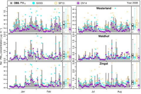
The modeled daily average sodium PM10 concentrations were compared with the concentrations measured at 11 EMEP stations. Figure 10 shows the sodium concentrations at three German EMEP stations (Westerland, Waldhof, and Zingst) in winter and summer. Table 3 reports the corre-sponding statistical data for all 11 stations. These stations in-clude both coastal and inland stations (see Table 2), whereas the Melpitz station is located far inland.
are not. GO03 overestimates the peak concentrations at West-erland and Zingst. The correlation coefficients for all three parameterizations are close to each other at both stations and in both seasons. However, the MNB is closest to 0 for the OV14 case, followed by GO03 and then SP13. The MNB of OV14 is typically negative, whereas it is positive for the other two cases. The RAE is highest for SP13, and the RAEs of GO03 and OV14 are similar. For all coastal stations in Table 3, the correlation coefficient decreases from winter to summer, whereas the MNBs and RAEs improve except for Westerland. At the station of Westerland in summer, the MNBs and RAEs are highest for SP13. At most coastal sta-tions, the MNBs for the SP13 and GO03 cases are positive and those for the OV14 case are negative. GO03 yielded the lowest RAEs and the MNBs closest to 0 at several of these stations, whereas OV14 yielded the highest RAEs. The latter is caused by high underestimations. The correlation coeffi-cients are quite similar and do not indicate a clear ranking. Notably, at Keldsnor (DK0005R), the correlation coefficients are particularly low.
At Waldhof, which is located approximately 200 km in-land, the modeled concentrations are closer to each other than at the other stations. In winter, SP13 and GO03 overes-timate several peak concentrations, but the baseline concen-trations are well reproduced by all three parameterizations. In summer, GO03 underestimates the baseline concentration and SP13 appears to yield the best reproduction of the obser-vations. Inland stations exhibit high correlation coefficients of between 0.6 and 0.8. The SP13 emissions yield the highest
correlation coefficients. However, their difference to the cor-relation coefficients of the GO03 and OV14 cases is small. In summer, the inland MNBs of the GO03 and SP13 cases are smaller than those at the coastal stations, indicating less overestimation of the sodium concentrations at inland sta-tions. For the OV14 case, the MNB is positive in approx-imately half of the inland cases – particularly during win-ter – whereas it is typically negative at all coastal stations. Thus, OV14 produces fewer underestimations at inland sta-tions. The RAE is often below 0.5 at inland stations, with the exception of Tange (DK0003R). Commonly, the winter MNB and RAE values are higher than those in summer. The MNBs and RAEs for Tange deviate most strongly from those for the other stations in this group. Tange is the station that is located closest to the coast. At Melpitz, the MNB of OV14 is positive in both winter and summer. In winter, the MNBs of SP13 and GO03 at Melpitz are lower than those at the other stations. Melpitz is also the station located the furthest from the coast line.
At the coastal station of Keldsnor (DK0005R), the cor-relation coefficients are very low. During winter, the RAEs are higher than those at the other stations. The RAEs during summer and the MNBs are in the same range as those at the other stations. Thus, the order of magnitude of the sodium concentrations is well reproduced, whereas the temporal oc-currences of the peak concentrations are not well reproduced
Figure 9.Similar to Fig. 7 but showing sea salt number emissions. (a–f)The 2-month average number emissions(g)box plots of num-ber emissions.
with respect to the other stations. Keldsnor is located on an island that is not resolved by the model, as is Anholt (DK0008R). However, Anholt is located on a small island that is surrounded only by water, whereas Keldsnor is located on a larger island in a region of several islands. Therefore, the local wind fields near Keldsnor may not be correctly pre-dicted, and consequently, sub-grid deposition processes may not be correctly reproduced by CMAQ, thereby causing the quality of the modeled sea salt concentrations to decline.
sim-● ●
OBS, PM10 GO03 SP13 OV14 Year 2008
OBS 0 2 4 6 8 10 ● ●●● ●● ● ●● ● ● ● ●● ● ● ● ● ● ● ● ●● ● ● ● ● ●●● ● ● ● ● ● ● ● ● ● ●●●●●● ●● ● ● ●● ● ● ● ● ● ● ● ● ● ● ●●● ● ● ● ● ● ● ● ● ● ● ● ● ● ● ● ● ● ● ● ● ● ●● ● ● ● ● ● ● ● ● ●● ●●●●●● ● ● ● ● ● ● ● ● ● ● ● 0 1 2 3 4 5 6 Westerland ● ●●●● ●● ● ●● ● ● ● ●● ● ● ● ● ● ● ● ● ●●●● ●●●●● ●●● ●●● ● ● ●●● ● ● ● ● ● ●● ● ● ●● ● ● ● ● ●● ● ● ● ● ●● ●● ● ● ● ● ● ● ●● ● ● ● ● ● ● ● ● ●●● ● ● ● ●●● ●●● ● ● ● ● ● ● ● ● ● ●● ● ● ● ● ● ● ● ● ● ● ● ● ● ● 0.0 1.0 2.0 3.0 N a P M c o n c e n tr a ti o n [ g m ] + 10 µ 3 ● ● ●●● ●● ● ●● ● ●● ●●●● ● ● ● ● ● ● ● ● ● ●● ● ●● ● ● ● ●● ● ● ● ● ● ● ● ●● ●● ● ● ● ●● ● ● ● ●● ● ● ● ● ● ●● ●● ● ● ● ● ● ●● ●●●● ● ● ● ● ● ● ● ● ●● ● ●● ● ● ●● ● ●●● ● ● ● ●●●● ●● ●● ● ● ● ●● ● ● ● 0.0 0.5 1.0 1.5 2.0 Waldhof ●●●●●●● ●● ●● ● ●●●● ● ●● ● ● ●● ● ●●●●●●●● ● ●● ● ●● ● ● ● ● ● ● ● ●●●●● ● ●● ●● ● ● ●●●● ●●●●●● ● ● ● ●● ● ● ● ● ● ● ● ● ● ● ● ● ● ● ●●●●●●● ● ● ● ● ● ● ● ● ● ● ● ● ● ●●●● ● ● ● ●● ● ● ●● ● ● 0 1 2 3 4 5 6 Jan Feb ●●●●● ●● ● ● ●● ●● ●●●● ● ● ● ●● ● ● ●● ● ● ●●● ● ● ● ●● ● ● ● ●● ● ● ● ● ● ● ● ● ● ● ● ● ● ●● ● ● ● ● ●●●●●● ● ● ● ● ● ● ● ●●●● ● ● ● ●● ● ● ● ● ●● ● ● ● ●● ● ● ●●● ● ●●● ● ● ● ● ● ● ● ● ● ● ● ● ● 0.0 1.0 2.0 3.0 Jul Aug Zingst ● ● ● ● ● ● ● ●● ● ● ●● ● ● ● ● ●● ● ●●●● ● ● ● ● ● ●● ● ● ● ●● ● ● ● ● ● ● ● ● ● ● ● ●● ● ● ● ● ● ●● ●●●● ● ● ● ● ● ●● ● ●● ● ● ● ● ● ● ● ● ●● ● ●● ●● ● ● ● ● ● ●● ● ● ● ● ● ● ● ● ● ● ● ● ● ● ● ●●● ● ● ● ● ● ●● ●● ● ● ● –
Figure 10.Sodium concentrations at three representative EMEP stations (Westerland, Waldhof and Zingst). The black box plot represents the observations. For the box plots of the modeled data, only the daily model values with corresponding measured values are considered.
ilar study, Tsyro et al. (2011) also reported slight overestima-tions at coastal staoverestima-tions and underestimaoverestima-tions at some inland stations for GO03 sea salt emissions. In that study, sodium concentrations calculated by the EMEP model were com-pared with EMEP data of the years 2004–2007. Comparing annual average concentrations over all stations yielded over-estimations. In contrast, a detailed evaluation (same study) of sodium PM10 and PM2.5 data of two EMEP intensive measurement campaigns from June 2006 and January 2007 showed that the model underestimated sodium concentra-tions in both size fracconcentra-tions at three of four EMEP staconcentra-tions. This result clearly contradicts the results of that study, which clearly highlights the temporal variability of sea salt emis-sions and indicates that either the emission or the transport processes are not correctly represented by the model. Chen et al. (2016) considerably overestimated sea salt concentra-tions in WRF-Chem model simulaconcentra-tions with GO03 sea salt emissions during a 2-week period in September 2013. The spatiotemporal variation of the concentrations was well cap-tured. Manders et al. (2010) compared particulate sodium concentrations predicted by the LOTOS-EUROS model with EMEP measurements for the year 2005. The sea salt emis-sions were generated by a combination of the emission pa-rameterizations by Monahan et al. (1986) and Mårtensson et al. (2003), which is similar to the SP13 parameterization. They found that the atmospheric annual mean sea salt con-centrations were approximately 2.6-fold overestimated com-pared to the EMEP measurements. In agreement with Chen et al. (2016), the spatiotemporal variation was well cap-tured. Moreover, the sea salt concentrations were reduced by 40–50 % when an alternative dry deposition parameteri-zation was employed. Both dry deposition parameteriparameteri-zations in Manders et al. (2010) and the parameterization used in
CMAQ are based on the classical resistance approach but the formulations of individual resistances differ. Therefore, a di-rect comparison of the dry depositions is not possible.
Another important aspect in sea salt modeling studies is the consideration of surf zone emissions: sea salt emissions are enhanced in the surf zone due to increased number of wave breaking events. The generation of surf zone emissions is a complex and small-scale process, which is very difficult to represent in models. Hence, it is commonly not considered in regional scale modeling studies. Kelly et al. (2010) and Gantt et al. (2015) optimized the surf zone emission treat-ment in CMAQ and found sodium and nitrate concentrations to be better predicted when surf zone emissions were con-sidered. Neumann et al. (2016) identified no improvement of modeled sodium concentrations when surf zone emissions were activated. In this study, the emissions by the GO03 and SP13 parameterizations incorporate surf zone emissions as suggested by Kelly et al. (2010), where those by OV14 in-corporate no surf zone emissions. The different treatment of surf zone emissions might also lead to an offset in the atmo-spheric sodium concentrations between GO03 and SP13, on the one side, and OV14, on the other side.
Table 3.Statistical evaluation for the comparisons between the modeled and measured Na+concentrations at 11 EMEP stations in the
vicinity of the North and Baltic seas during winter (left) and summer 2008 (right).
sodium PM10 Winter 2008 Summer 2008
Station Case n RAE MNB R n RAE MNB R
Westerland GO03 60 1.62 0.80 0.77 61 0.64 1.90 0.69
Coast SP13 60 2.87 1.05 0.75 61 1.09 2.79 0.71
DE0001R OV14 60 2.23 −0.37 0.75 61 1.01 −0.12 0.70
Zingst GO03 60 0.60 1.01 0.77 61 0.26 0.02 0.70
Coast SP13 60 1.01 1.16 0.80 61 0.36 0.47 0.59
DE0009R OV14 60 0.64 −0.11 0.77 61 0.43 −0.57 0.76
Keldsnor GO03 60 1.09 0.59 0.45 56 0.43 0.04 0.26
Coast SP13 60 1.58 0.59 0.61 56 0.56 0.30 0.33
DK0005R OV14 60 1.32 −0.51 0.46 56 0.76 −0.64 0.37
Anholt GO03 59 1.02 0.35 0.81 51 0.64 −0.10 0.67
Coast SP13 59 1.87 0.61 0.82 51 0.69 0.12 0.66
DK0008R OV14 59 1.63 −0.54 0.70 51 1.07 −0.67 0.58
Utö GO03 59 0.46 1.00 0.59 61 0.26 0.09 0.66
Coast SP13 59 1.12 2.07 0.65 61 0.26 0.73 0.62
FI0009R OV14 59 0.32 0.21 0.61 61 0.34 −0.31 0.57
Ulborg GO03 60 1.14 1.44 0.74 54 0.58 0.99 0.50
Coast SP13 60 1.96 0.84 0.84 54 0.76 0.78 0.78
DK0031R OV14 60 1.35 −0.34 0.79 54 0.62 −0.41 0.71
Virolahti II GO03 60 0.21 1.30 0.34 54 0.10 0.05 0.74
Coast SP13 60 0.35 2.08 0.45 54 0.11 0.87 0.73
FI0017R OV14 60 0.18 0.72 0.33 54 0.13 0.33 0.55
Tange GO03 56 0.87 0.92 0.67 61 0.40 0.64 0.62
Inland SP13 56 1.37 1.00 0.77 61 0.58 0.93 0.73
DK0003R OV14 56 0.97 −0.23 0.73 61 0.45 −0.32 0.67
Waldhof GO03 55 0.39 1.62 0.65 60 0.20 −0.42 0.70
Inland SP13 55 0.47 1.80 0.73 60 0.19 0.15 0.71
DE0002R OV14 55 0.40 0.63 0.73 60 0.20 −0.34 0.68
Neuglobsow GO03 60 0.28 1.13 0.75 59 0.19 −0.45 0.72
Inland SP13 60 0.36 1.22 0.83 59 0.14 0.15 0.71
DE0007R OV14 60 0.36 0.41 0.75 59 0.20 −0.32 0.64
Melpitz GO03 59 0.25 0.30 0.66 61 0.12 −0.41 0.70
Inland SP13 59 0.27 0.81 0.67 61 0.10 0.43 0.67
DE0044R OV14 59 0.27 0.10 0.63 61 0.13 0.11 0.57
sodium concentrations are evaluated to explain the results of this section in more detail.
3.2.2 Particle size distribution
In this section, the sea salt particle size distributions in the GO03, SP13, and OV14 cases and their evolution from their source regions toward inland are analyzed. This is performed by considering the PM2.5 and PMC sodium concentrations
(PMC=PM10−PM2.5) at the Westerland (coast) and
Mel-pitz (inland) stations. In addition, the modeled PM2.5 and
PMC sodium data are compared with measurements at the Melpitz station. This comparison is presented first (Fig. 11) followed by an evaluation of the modeled sodium PM data at both stations (Fig. 12). For more detailed considerations, the PM2.5 and PMC sodium data at Waldhof, which is lo-cated at approximately half of the distance between Wester-land and Melpitz, and the modeled accumulation and coarse-mode GMDs at the Westerland, Waldhof, and Melpitz sta-tions are provided in the Supplement (Figs. S8 and S9).
concentra-● ●
OBS, PM10−2.5 OBS, PM2.5 GO03 SP13 OV14 Melpitz 2008
● ● ●●●● ● ● ●●●●●●●●●● ● ● ● ● ● ● ● ● ● ● ●● ●● ● ● ●● ● ● ● ● ●●●●●● ● ● ● ● ● ● ● ● ● ●● ● ● ● ● ● ●●●● ● ● ● ●● ●● ●●●● ● ● ● ● ● ●● ● ● ● ● ● ● ● ● ●● ● ● ●●●●● ●● ● ● ● ● ● ● ● ●● ● ● 0.0 0.5 1.0 1.5 2.0 ● ● ●●●● ●● ●●●●●●●●●●●● ● ● ● ●● ● ● ●● ● ●● ● ● ● ● ● ● ● ● ●●●●● ●● ●● ● ● ● ● ● ● ●● ● ● ● ● ● ●●●● ●● ● ●● ●● ●●●● ● ● ● ● ● ● ● ● ● ● ●● ● ●● ● ● ● ● ● ●● ● ● ●●●● ●● ●● ● ● ● ● ● ● ●● ● ● ● 0.0 0.2 0.4 0.6 Na +c o n c e n tr a ti o n [ g m ] µ 3 ● ●●●●● ● ● ●●●●●●●●● ● ● ●● ● ●● ● ● ● ● ●● ●● ● ● ●● ● ● ● ● ●●●●●●● ● ● ● ● ● ● ● ● ●● ● ● ● ● ●●●●● ● ● ● ●●●●●●●● ● ● ● ● ● ●● ● ● ● ●● ● ● ● ● ● ● ● ●●●●●●● ● ●● ● ● ● ● ●● ● ● ● Jan Feb 0.0 0.5 1.0 1.5 2.0 ●●●●● ●● ● ● ● ●●● ●● ● ● ●● ● ● ●● ●●●●●●●●● ● ●● ● ● ● ● ● ●●● ● ● ● ● ● ● ● ●● ● ● ● ● ● ●●●● ●●●● ● ● ● ● ● ● ● ●● ●● ● ● ●● ● ●● ● ● ●●●●●●● ● ● ● ● ● ● ● ● ● ● ● ●● ●● ● ● ● ● ● ● ● ● ●● ● ● 0.0 0.2 0.4 0.6
0.8 PM10
●●●●●● ●● ● ●●●● ●● ● ● ●●● ● ● ● ● ●●●●●●●●●●●●●●● ● ● ●● ● ● ●●●● ●●●●●● ● ●●●●● ●●●● ●● ●● ● ● ● ●●● ● ● ● ●● ● ● ● ● ● ● ●●●●●●● ●● ● ● ● ●● ● ● ● ● ● ● ●●●● ● ● ● ●● ● ●● ●●● 0.0 0.1 0.2 0.3 0.4 PM 2.5 ●●●●●●● ● ● ●●●● ● ●● ● ●● ● ● ● ● ●●●●●●●●● ● ●● ● ● ● ● ● ●●● ● ● ● ● ● ● ● ●● ● ● ● ● ● ●●●● ●●●● ● ●● ● ● ●●●● ●● ● ● ●● ● ● ● ● ●●●●●●●●● ● ●● ● ● ● ● ●●● ● ● ● ● ●● ● ● ● ● ● ● ● ● ●● ● ● Jul Aug 0.0 0.2 0.4 0.6 0.8 PM C –
Figure 11.Daily average measured and modeled sodium concentrations at the EMEP station at Melpitz. The sodium PM10, PM2.5and PMC concentrations are plotted in the top, center and bottom rows, respectively, for winter (left) and summer (right). The black box plot represents the observations. For the box plots of the modeled data, only the daily model values with corresponding measured values are considered.
tions with respect to their magnitude. SP13 and OV14 yield considerable overestimations. During winter, all parameteri-zations underestimate the sodium PM2.5peak concentrations, but SP13 overestimates the baseline concentrations, and pos-itive MNBs indicate overestimations in all three cases. The average concentrations are best predicted by OV14, but the MNB is lowest for GO03. The correlation coefficient for OV14 is lower than those for GO03 and SP13 (Table 4). Thus, GO03 produces the best sodium PM2.5 predictions, followed by OV14. Because OV14 is based on a highly de-tailed particle size distribution data set and considers ultra-fine particles (the Aitken mode), it might be expected that this parameterization would yield the best predictions of the sodium PM2.5particle concentrations.
The temporal occurrences of peak sodium PMC concentra-tions are not consistently predicted by the three parameteriza-tions; i.e., GO03 and SP13 predict several peaks that are not predicted by OV14, and OV14 also predicts peaks that are not predicted by the other two cases. The sodium PMC con-centrations are underestimated by all three cases in summer (MNB<0), which leads to underestimation of the sodium
PM10concentrations by GO03. OV14 and SP13, in contrast, still moderately overestimate the sodium PM10 concentra-tions because of a considerable overestimation of sodium PM2.5. In particular, OV14 considerably overestimates the sodium PMCconcentrations in late August for approximately a week, whereas the other parameterizations predict lower and more accurate concentrations. If this period were to be neglected, a more pronounced negative MNB for OV14 dur-ing summer would occur. In winter, the coarse particles are overestimated by all parameterizations (MNB>0); this
over-estimation is lowest for OV14 and highest for SP13. The
cor-relation coefficients and RAEs for each season are quite sim-ilar and provide no clear indication of which parameteriza-tion yields better results. Thus, based on theR values and
the RAEs, no parameterization produces a clearly superior prediction of sodium PMCconcentrations. According to the MNBs, OV14 produces slightly better results than the other two cases when winter and summer are considered together. In summary, GO03 produces the best sodium PM2.5 con-centrations, and OV14 produces the best sodium PMC con-centrations at Melpitz. This size-resolved comparison indi-cates that sodium PM10 concentrations are not necessarily appropriate for validating sea salt emission parameterizations but that size-resolved measurements are of considerable im-portance in the validation process. Therefore, size-resolved sodium measurements in coastal regions will be necessary for the further evaluation of sea salt source functions.
For evaluating the evolution of the sodium size distribu-tions from the coast toward the hinterland, Fig. 12 depicts similar data as Fig. 11 but at the Westerland station. The same plot is presented in Fig. S9 in the Supplement for Wald-hof, which is located in between Westerland and Melpitz. At Westerland, PMCsodium represents the predominant contri-bution to the total sodium mass in all three sea salt emission parameterizations (Fig. 12). The sodium PM2.5 and PMC concentrations are twice as high during winter than sum-mer. The SP13 case yields the highest sodium PMC con-centrations, and OV14, yields the lowest. By contrast, the OV14 case yields higher sodium PM2.5concentrations than
the GO03 case in summer. In winter, the sodium PM2.5
●GO03 ●SP13 OV14 Westerland 2008 ● ● ●● ● ● ● ●● ● ● ●●●● ● ●● ● ● ● ● ● ● ● ● ● ● ●● ● ● ● ● ● ● ● ● ● ● ● ●●●● ●●● ● ● ● ● ● ● ● ● ● ● ● ● ● ● ●● ● ● ● ●● ● ● ● ●● ● ● ● ● ● ● ●● ● ●● ● ● ● ● ● ● ●● ● ●● ●●● ●●● ● ●● ● ● ● ● ● ● ● ● ● ● 0.0 0.2 0.4 0.6 Na +c o n c e n tr a ti o n [ g m ] µ 3 ● ●●● ●● ● ●● ● ● ● ●● ● ● ● ● ● ● ● ●● ● ● ● ● ●●● ● ● ● ● ● ● ● ● ● ●●●●●● ●● ● ● ● ● ● ● ● ● ● ● ● ● ● ● ●●● ●● ● ● ● ● ● ● ● ● ● ● ● ● ● ● ● ● ● ● ●● ● ● ● ● ● ● ● ● ●●●●●●●● ● ● ● ● ● ● ● ● ● ● ● Jan Feb 0 2 4 6 8 10 ● ●● ●● ● ● ● ● ● ● ● ●●● ● ● ●● ● ● ● ● ● ●● ●●●●●●●●●●●● ● ● ● ● ● ● ●● ● ●●●● ● ●●●●● ● ●● ● ●● ● ● ● ●●● ●● ● ● ● ●● ● ● ● ● ● ● ●● ●● ● ● ● ●● ● ●● ● ● ● ● ● ● ●● ● ●● ● ● ● ● ● ● ● ● ● ●● ● ● ● ● 0.0 0.2 0.4 0.6 PM 2.5 ● ●●●● ●● ● ●● ● ● ● ●● ● ● ● ● ● ● ● ● ●●●●●●●●● ●●● ●●● ● ● ● ●● ● ● ●● ● ● ● ● ● ●● ● ● ● ● ●● ● ● ● ● ●● ●● ● ● ● ● ● ● ●● ● ● ● ● ● ● ● ● ●● ● ● ● ●●● ●●● ● ● ● ● ● ● ● ● ● ●● ● ● ● ● ● ● ● ● ● ● ● ● ● ● Jul Aug 0 1 2 3 4 5 6 PMC –
Figure 12.Similar to Fig. 11 but showing data for Westerland. No sodium PM2.5data were available and no sodium PMCconcentrations were calculated.
Table 4.Similar to Table 3 but for the Melpitz station only and for different particle sizes.
Sodium PMx winter summer
Size Case n RAE MNB R n RAE MNB R
PM10 GO03 59 0.25 0.43 0.66 61 0.11 −0.35 0.69
SP13 59 0.39 1.27 0.67 61 0.12 0.58 0.67
OV14 59 0.27 0.11 0.65 61 0.13 0.12 0.57
PM2.5 GO03 58 0.09 0.19 0.64 56 0.03 0.08 0.50
SP13 58 0.10 1.37 0.64 56 0.07 2.28 0.45
OV14 58 0.10 0.39 0.52 56 0.06 1.27 0.31
PMC∗ GO03 56 0.20 0.69 0.64 52 0.11 −0.40 0.53
SP13 56 0.35 1.42 0.65 52 0.13 0.15 0.50
OV14 56 0.19 0.19 0.65 52 0.11 −0.27 0.48
∗Sodium PMCis calculated as PM10−PM2.5of sodium. In rare situations, PM10<PM2.5exists in the
measurements. In these situations, the resulting PMCvalue is not considered.
concentrations at Waldhof are middling (Supplement). The decrease in the sodium PM2.5concentrations from Wester-land via Waldhof to Melpitz is lower compared to the de-crease in sodium PMC concentrations. Therefore, the rele-vance of the PM2.5 sea salt fraction increases with distance to the marine sea salt emission regions. Fine particulate sea salt is more relevant for the transport of species attached to the particles over long distances, such as nitrate. In contrast, coarse sea salt particles are the size fraction predominantly deposing close to their source regions and enhance the depo-sition flux of attached species, such as nitrogen compounds. Hence, sea salt emission parameterizations that include more fine particles, such as OV14, can be expected to transport higher concentrations of those attached species over long dis-tances than parameterizations that yield a strong dry deposi-tion close to source regions, such as SP13. The different dry deposition velocities are not only due to a different split of the sea salt mass between accumulation and coarse mode but also due to different GMDs of the modal distributions. Plots of accumulation and coarse-mode GMDs that clearly
high-light the differences between the sea salt emission cases are provided in the Supplement but are not discussed.
3.3 Wet deposition
Modeled sodium wet deposition of the three sea salt emis-sion cases and sodium wet deposition measurements were compared. Measurements from 14 of more than 30 available stations were chosen for this comparison because the number of measurements per 2-month period was above 10 and the stations were not located on high mountains.
Table 5.Statistical metrics on modeled and measured sodium wet deposition at 14 EMEP stations. RAE, MNB,R,µP(mean predicted), and µO(mean observed) are shown.
Sodium wet deposition Winter 2008 Summer 2008
Station Case n RAE MNB R µP µO n RAE MNB R µP µO
Råö GO03 38 0.229 −0.545 0.560 0.071 0.294 26 0.047 −0.397 0.338 0.031 0.069
SE0014R SP13 38 0.164 −0.036 0.574 0.192 0.294 26 0.057 −0.081 0.359 0.054 0.069
Coast OV14 38 0.273 −0.857 0.548 0.021 0.294 26 0.060 −0.812 0.359 0.010 0.069
Leba GO03 31 0.028 0.568 0.374 0.024 0.037 28 0.017 −0.752 0.598 0.006 0.024
PL0004R SP13 31 0.045 1.907 0.410 0.056 0.037 28 0.012 −0.574 0.618 0.013 0.024
Coast OV14 31 0.031 −0.168 0.374 0.009 0.037 28 0.018 −0.776 0.570 0.006 0.024
Preila GO03 20 0.101 −0.613 0.206 0.034 0.115 29 0.065 −0.318 −0.170 0.006 0.067
LT0015R SP13 20 0.134 −0.016 0.253 0.090 0.115 29 0.066 0.436 −0.152 0.014 0.067
Coast OV14 20 0.100 −0.825 0.217 0.015 0.115 29 0.067 −0.037 −0.174 0.007 0.067
Rucava GO03 18 0.053 −0.379 0.358 0.037 0.062 30 0.020 −0.666 0.254 0.003 0.024
LV0010R SP13 18 0.074 0.495 0.364 0.093 0.062 30 0.018 −0.408 0.281 0.007 0.024
Coast OV14 18 0.046 −0.689 0.391 0.017 0.062 30 0.020 −0.784 0.386 0.003 0.024
Birkenes GO03 37 0.250 −0.714 0.399 0.074 0.324 27 0.099 −0.127 0.553 0.023 0.113
NO0001R SP13 37 0.210 −0.284 0.395 0.214 0.324 27 0.099 0.364 0.518 0.043 0.113
Mixed OV14 37 0.301 −0.902 0.388 0.023 0.324 27 0.105 −0.685 0.499 0.009 0.113
Kårvatn GO03 31 0.191 −0.750 0.161 0.007 0.197 24 0.031 − −0.336 0.025 0.022
NO0039R SP13 31 0.184 −0.524 0.195 0.016 0.197 24 0.033 − −0.199 0.023 0.022
Coast OV14 31 0.194 −0.886 0.183 0.002 0.197 24 0.020 − −0.043 0.007 0.022
Tustervatn GO03 36 0.214 −0.710 0.224 0.015 0.216 22 0.011 − 0.055 0.012 0.004
NO0015R SP13 36 0.232 −0.410 0.222 0.037 0.216 22 0.018 − 0.022 0.018 0.004
Inland OV14 36 0.212 −0.874 0.225 0.005 0.216 22 0.005 − 0.046 0.004 0.004
Waldhof GO03 19 0.025 0.652 0.375 0.025 0.028 30 0.007 −0.411 0.083 0.002 0.009
DE0002R SP13 19 0.050 2.491 0.411 0.055 0.028 30 0.007 −0.016 0.067 0.004 0.009
Inland OV14 19 0.020 −0.401 0.282 0.009 0.028 30 0.008 −0.651 0.114 0.001 0.009
Neuglobsow GO03 22 0.010 0.212 0.546 0.016 0.016 22 0.010 −0.508 −0.082 0.002 0.012
DE0007R SP13 22 0.025 1.609 0.532 0.035 0.016 22 0.011 −0.075 −0.079 0.004 0.012
Inland OV14 22 0.011 −0.613 0.503 0.005 0.016 22 0.010 −0.673 0.035 0.001 0.012
Zoseni GO03 12 0.031 −0.642 0.580 0.012 0.041 29 0.004 −0.793 0.146 0.001 0.005
LV0016R SP13 12 0.028 −0.155 0.580 0.032 0.041 29 0.004 −0.563 0.132 0.002 0.005
Inland OV14 12 0.036 −0.839 0.545 0.005 0.041 29 0.004 −0.776 0.148 0.001 0.005
Diabla Gora GO03 21 0.025 −0.245 0.597 0.023 0.034 25 0.004 −0.799 0.465 0.001 0.005
PL0005R SP13 21 0.047 0.670 0.597 0.058 0.034 25 0.004 −0.586 0.460 0.002 0.005
Inland OV14 21 0.026 −0.743 0.596 0.008 0.034 25 0.004 −0.818 0.511 0.001 0.005
Løken GO03 32 0.029 −0.146 0.425 0.017 0.034 25 0.031 4.257 0.226 0.005 0.034
NO0218R SP13 32 0.039 0.572 0.454 0.037 0.034 25 0.031 6.477 0.231 0.008 0.034
Inland OV14 32 0.030 −0.722 0.386 0.005 0.034 25 0.032 0.518 0.222 0.002 0.034
Hurdal GO03 26 0.052 −0.976 0.427 0.001 0.053 28 0.022 −0.589 0.390 0.006 0.025
NO0056R SP13 26 0.051 −0.948 0.411 0.002 0.053 28 0.022 −0.291 0.476 0.012 0.025
Inland OV14 26 0.053 −0.993 0.431 0.000 0.053 28 0.022 −0.840 0.397 0.002 0.025
Jarczew GO03 24 0.007 −0.398 0.300 0.007 0.009 17 0.004 −0.919 −0.296 0.000 0.004
PL0002R SP13 24 0.015 0.326 0.303 0.016 0.009 17 0.004 −0.827 −0.296 0.001 0.004