Atmos. Chem. Phys., 9, 7657–7677, 2009 www.atmos-chem-phys.net/9/7657/2009/ © Author(s) 2009. This work is distributed under the Creative Commons Attribution 3.0 License.
Atmospheric
Chemistry
and Physics
Reactive nitrogen in atmospheric emission inventories
S. Reis1, R. W. Pinder2, M. Zhang3, G. Lijie4, and M. A. Sutton1
1Centre for Ecology & Hydrology (CEH), Bush Estate, Penicuik, EH26 0QB, UK
2US Environmental Protection Agency, Atmospheric Modeling Division, 109 T W Alexander Drive, Research Triangle Park,
NC 27711, USA
3Institute of Atmospheric Physics, Chinese Academy of Sciences, Beijing, China
4The College of Environmental Science and Engineering, Nankai University, Tianjin, 300071, China
Abstract. Excess reactive Nitrogen (Nr) has become one of the most pressing environmental problems leading to air pol-lution, acidification and eutrophication of ecosystems, bio-diversity impacts, leaching of nitrates into groundwater and global warming. This paper investigates how current inven-tories cover emissions of Nr to the atmosphere inEurope, the United States of America, andChina. The focus is on anthro-pogenic sources, assessing the state-of-the-art of quantifying emissions of Ammonia (NH3), Nitrogen Oxides (NOx) and
Nitrous Oxide (N2O), the different purposes for which
inven-tories are compiled, and to which extent current inveninven-tories meet the needs of atmospheric dispersion modelling. The paper concludes with a discussion of uncertainties involved and a brief outlook on emerging trends in the three regions investigated is conducted.
Key issues are substantial differences in the overall mag-nitude, but as well in the relative sectoral contribution of emissions in the inventories that have been assessed. While these can be explained by the use of different methodologies and underlying data (e.g. emission factors or activity rates), they may lead to quite different results when using the emis-sion datasets to model ambient air quality or the deposition with atmospheric dispersion models. Hence, differences and uncertainties in emission inventories are not merely of aca-demic interest, but can have direct policy implications when the development of policy actions is based on these model results.
The level of uncertainty of emission estimates varies greatly between substances, regions and emission source sec-tors. This has implications for the direction of future research needs and indicates how existing gaps between modelled and measured concentration or deposition rates could be most ef-ficiently addressed.
Correspondence to:S. Reis ([email protected])
The observed current trends in emissions display decreas-ing NOx emissions and only slight reductions for NH3 in
both Europe and the US. However, in China projections in-dicate a steep increase of both.
1 Introduction
1.1 Aims and objectives
Nitrogen gas (N2) accounts for more than 99.99% of all the
nitrogen present in the atmosphere, while of the rest, again 99% is accounted for by nitrous oxide (N2O) (Wallace and
Hobbes, 2006). Other N species are thus only present in trace concentrations, but nonetheless play a vital role in at-mospheric chemistry. Ammonia (NH3) is the most abundant
alkaline gas in the atmosphere and is responsible for neu-tralising acids formed through the oxidation of sulphur diox-ide (SO2) and nitrogen oxides (NOx), creating ammonium
(NH+4) salts of sulphuric and nitric acid, which become mospheric aerosols. The only other alkaline gases in the at-mosphere are also reduced nitrogen, such as volatile amines, though these are present in much smaller quantities. Oxi-dized nitrogen, mainly originating as nitric oxide (NO) and nitrogen dioxide (NO2) plays a crucial roles both in
tropo-spheric and stratotropo-spheric chemistry, for instance in the for-mation of tropospheric ozone (see Bradshaw et al., 2000; Brasseur et al., 1999).
Nitrogen is thus present in the atmosphere in a multiplicity of chemical forms, contributing both the majority (78%) of the atmosphere as N2and a plethora of trace N components
that are fundamental to the atmosphere’s chemical and radia-tive properties. It is convenient to distinguish these N forms into two main groups: N2 being termed non-reactive (or
“fixed”) nitrogen, with the sum of all other N forms present being termed “reactive nitrogen” (Nr) (Galloway et al., 2003, 2008).
The amounts of Nr in the world are of fundamental im-portance to society. Since the invention of the Haber-Bosch process it has become possible to synthesise huge amounts of NH3 directly from N2. The key benefit has been to feed
the increasing world population, which is offset by the conse-quent increases in Nr losses to the environment (e.g. Erisman et al., 2008). In parallel, high temperature combustion of fos-sil fuels oxidizes atmospheric N2, causing a huge increase in
NOx emissions in the atmosphere (Lee et al., 1997). The
alteration in agricultural practice and increase in fossil fuel combustion impacts human health, acidification and eutroph-ication of soils, biodiversity change in terrestrial ecosystems, nitrate eutrophication in freshwater and marine ecosystems and affects the global radiative balance. Furthermore, N2O
emissions are not only contributing to global warming with a significantly higher global warming potential than CO2
and CH4, but have recently been identified to substantially
contribute to stratospheric ozone depletion on a global scale (Ravishankara, 2009). And as N2O emissions from
agricul-tural soils are closely linked to NH3emissions from fertilizer
and manure application, it is sensible to address N2O
emis-sions in the context of this study, even though N2O is
typi-cally not classed as reactive nitrogen (Nr).
While there is sufficient evidence to demonstrate the sub-stantial perturbation of the global nitrogen cycle, the exact quantification of the magnitude and spatial distribution of this perturbation is presently subject to in-depth research. The NitroEurope research project (Sutton et al., 2007; http:// www.nitroeurope.eu) is working towards deriving more pre-cise nitrogen balances from local to regional scales. A ma-jor challenge in compiling nitrogen budgets and quantifying pools and fluxes of nitrogen in the atmosphere and biosphere is that models and measurements need to be of good and known quality to allow for a validation of results and ulti-mately provide the scientific understanding of processes on all relevant spatial scales. The variety of sources of different forms of nitrogen being emitted into the atmosphere, soils and water bodies, their heterogeneous distribution in space and the often high uncertainties regarding specific N fluxes creates a challenge for the validation and verification of mod-els. At present, closing the gaps in the nitrogen budgets is the aim of major efforts on a global scale. One example for this is the European Nitrogen Assessment Report (compiled un-der the auspices of the ESF Programme Nitrogen in Europe and the International Nitrogen Initiative), which is due to be completed by early 2011 and which aims to improve the un-derstanding of the European N cycle and move towards clos-ing the gaps. Emission inventories are a critical source of in-formation in this process. They are most often compiled for compliance monitoring purposes, e.g. EMEP under the UN-ECE Convention on LRTAP or the United Nations Frame-work Convention on Climate Change (UNFCCC), using of-ficially submitted data compiled by country experts. Other inventories are compiled by researchers with the main aim to provide a consistent and comprehensive set of input data
for modelling purposes (e.g. the EDGAR datasets, IIASA GAINS), often using a bottom-up approach with informa-tion on emission factors and activity data that are publicly accessible.
In this paper, we focus on regional scale nitrogen emission inventories for the year 2005, with the aim to assess how different methods and data sources influence the resulting inventory datasets. In a second step, we analyse the main drivers for differences identified, and consider how these may affect the usefulness of datasets for atmospheric mod-elling. Finally, we briefly discuss emission trends from in-ventory datasets and scientific literature, considering the im-plications for our conclusions on the use of emission datasets for modelling purposes.
1.2 Scope
Anthropogenic activities have a significant impact on the magnitude of N cycled and released into the atmosphere (see Table 1), for instance, Galloway et al. (2004) calculated a global rate of annual creation of reactive nitrogen (Nr) of 163 Tg N yr−1in the early 1990s, compared to 125 Tg N yr−1 around 1860.
The following Table 2 displays the total N emissions in Tg for the three regions on which this paper focuses. It illus-trates both the similarities and differences between different inventories and the contribution to the atmospheric domain of global N emissions, which based on the EDGAR v4 in-ventory (EDGAR, 2009) amounts to approx. 32 Tg N in the year 2005.
At the same time, the scientific understanding of many environmental effects of excess nitrogen in the atmosphere has significantly advanced in recent years. Current research into the critical loads of N deposition both for acidification and eutrophication (see Hettelingh et al., 2008) has led to the establishment of more stringent critical loads, with dy-namic modelling approaches being explored to assess the timescales of ecosystem damage and recovery. In addition, the relevance of N2O as a contributor to global warming has
been acknowledged and emission control strategies no longer focus solely on CO2, which is reflected e.g. by a more
de-tailed integration of N2O sources and measures in the GAINS
model (Greenhouse Gas – Air Pollution Interaction an Syn-ergies, http://gains.iiasa.ac.at/) or MITERRA (Velthof et al, 2009).
Given the importance of nitrogen-containing species for air quality and climate change, the question emerges if to-day’s inventories of NH3, NOxand N2O reflect the current
S. Reis et al.: Reactive nitrogen in atmospheric emission inventories 7659
Table 1.Overview of the main sources and sinks of atmospheric nitrogen-containing species. N2has been listed for completeness, but is not discussed further, as the paper focuses on reactive N species only.
Sources (N2) NH3 NOx N2O
Biogenic emissions from the terrestrial and marine biosphere X X X
Decomposition of proteins and urea from animals X
Biomass burning and fossil fuel combustion (X) X X
Agricultural mineral Nr fertilisation and denitrification (X) X X X
Lightning X
Sinks
Wet deposition (as NH+4 and NO−3) X X
Dry deposition X X
Biological nitrogen fixation (X)
Industrial nitrogen fixation (mainly Haber-Bosch process) (X)
Chemical breakdown in the stratosphere X
Table 2.Emissions in Tg Nitrogen (Tg N) for the three regions analysed in this paper based on a global inventory (EDGAR v4) and national submissions (to EMEP, IPCC) for the year 2005. In the case of the China, no official national inventory was available; NH3emissions as estimated for 2006 by Yan et al. (2003) and other data from the IIASA GAINS China model have been used for the comparison. The last column shows global figures of Tg N emitted based on the EDGAR v4 dataset, as well as the share of emissions of the three regions investigated contributing to global emissions in brackets anditalics.
EU25a USA China Global
EDGAR v4 EMEP1/IPCC2 EDGAR v4 US EPA EDGAR v4 IIASA3/Yan et al. 20034 EDGAR v4
NH3 4.35 3.301 2.81 3.02 8.43 5.804 33.4(46.7%)
NOx 3.51 3.491 5.48 5.61 5.59 5.203 28.1(51.8%)
N2O 0.63 0.822 0.46 0.65 0.68 1.183 3.9(45.1%)
8.48 7.61 8.75 9.28 14.69 12.18 65.4(48.8%)
aEU27, except Malta and Cyprus, omitted for consistency with figures.
has led to different accounting systems with often differing national budgets for the same trace gas. In this paper, we compare how different approaches to inventory compilation may lead to similar or quite different results and – where possible – discuss likely reasons for differences observed. Specifically, we assess whether the quality of current emis-sion inventories is sufficient to support integrated strategies for N management, which are emerging in the US and Eu-rope (Erisman et al., 2007). For this purpose, we here assess existing inventories with regard to their total numbers and sectoral structure. Thetemporalandspatial resolution, spe-ciationandaccessibility of inventoriesare not the focus of this paper, but will be addressed where necessary.
In the following sections, the current situation of emission inventories in Europe, the US and China is discussed with the focus on how emissions of NH3, NOxand N2O are
es-timated and allocated to source sectors. Aspects of spatial and temporal resolution, sectoral detail on emission sources and completeness of reporting are addressed for the legisla-tive and regulatory regimes under which data are compiled. Where different inventories are compiled, a comparison and
analysis of potential variations will be conducted, alongside uncertainty assessments.
For this purpose, the following inventories and data sources have been analysed in detail:
– National submissions of NOxand NH3emission date to
the EMEP programme
– National submissions of N2O emission data to the
UN-FCCC/IPCC
– The US National Emissions Inventory (NEI) dataset for NOxand NH3
– Inventory of US Greenhouse Gas Emissions and Sinks for N2O
– The EDGAR global emission inventory dataset for NOx, NH3 and N2O (version 4 representing the most
up-to-date emissions; EDGAR Fast Track 32 and EDGAR HYDE for trends and for comparison pur-poses)
– Literature data in particular for the China and for global/regional comparisons.
The datasets listed are openly accessible, in most cases di-rectly online. The EDGAR v4 inventory (EDGAR, 2009) has only been partly published at this stage (greenhouse gases). However, the authors had access to a preliminary version of the dataset for air pollutants, which will be pub-lished in the near future, subject to error corrections to which the comparisons made in this paper may contribute (http://edgar.jrc.ec.europa.eu/). For an overview over all data sources and URLs, see Table 3.
On a global scale, the need for nitrogen management has been formulated in the 2004 Nanjing Declaration (Erisman 2004, UNEP 2004), which was presented to theUnited Na-tions Environment Programme(UNEP) in Nanjing, China on October 16, 2004, with the aim to optimise nitrogen manage-ment in food and energy production on a local, regional and global scale.
2 European emission inventories of reactive nitrogen species
In Europe, emissions of ammonia and nitrogen oxides are covered by several regulatory regimes, both under the UN-ECE CLRTAP and directives of the European Commission. Member states of the European Union and parties to the pro-tocols under the CLRTAP are subject to mandatory emission reporting. For the UNECE, the EMEP Centre on Emission Inventories and Projections (CEIP) at the Umweltbundesamt Vienna, Austria, hosts inventory datasets (both official sub-missions of signatories to the different protocols of the CLR-TAP and emissions for modelling purposes) in an online-accessible database (http://www.ceip.at/).
Nitrous oxide on the other hand is not covered by the CLR-TAP, but is required to be reported under the UNFCCC by Table 3 countries. The UNFCCC GHG inventory submis-sions can be accessed http://unfccc.int/ghg emissubmis-sions data/ items/3800.php online.
In addition to these inventories which are generated based on obligatory reporting of national emissions, the EDGAR database provided global annual emissions per country and on a 1×1 degree grid for 1990 and 1995 for direct green-house gases CO2, CH4, N2O and HFCs, PFCs and SF6 and
the precursor gases CO, NOx, NMVOC and SO2. Similar
inventories have been compiled for acidifying gases, NH3,
NOx and SO2 and Ozone Depleting Gases (EDGAR v4 as
well as EDGAR 3.2/FT 2000, see EDGAR, 2009). For this paper, the new EDGAR dataset version 4 (v4 in the fol-lowing text) is used, which has recently been (partly, for GHGs) officially released and of which a preliminary ver-sion was made available to the authors by the EDGAR team (http://edgar.jrc.ec.europa.eu/). EDGAR v4 (EDGAR, 2009) provides emissions for all relevant air pollutants and GHGs with an improved spatial resolution and until 2005.
0 100 200 300 400 500 600 700 800
Au
s
tr
ia
Be
lgium
Bu
lgaria
C
z
ec
h R
e
public
De
n
m
a
rk
Est
onia
Fin
land
Fra
n
ce
Germ
any
Gre
e
ce
Hunga
ry
Ire
land Italy
La
tv
ia
Lithu
ania
L
u
xembourg
N
e
therla
nds
Po
land
Po
rtuga
l
Ro
ma
n
ia
Slo
v
akia
Slo
v
enia
S
pain
Sweden
United
King
dom
Gg N
EMEP IIASA EDGAR v4
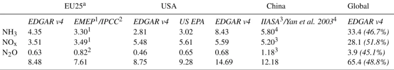
Fig. 1.Comparison of EU27 (not showing Malta and Cyprus)
emis-sions of ammonia (expressed in Gg N) reported to EMEP and com-piled by IIASA and the EDGAR v4 database for the year 2005. The slight differences between IIASA estimates and EMEP figures arise most likely from bilateral consultations with country experts, which led to corrections in agricultural emissions that had not (yet) been reflected in the EMEP inventories by recalculations of the year 2000 emissions submitted.
2.1 Ammonia
In the case of NH3, the vast majority of emissions from the 27
member states of the European Union (EU27) originate from agriculture (93%), with some small contributions from waste management (2.5%), industrial production processes (2%) and road transport (1.8%) (EMEP, 2009). This sectoral dis-tribution is valid for most countries, with slight difference de-pending on the state of the art of agricultural production and, for instance, livestock intensity. For ammonia, a large num-ber of non-agricultural sources contribute a small amount of emission (Sutton et al., 2000). Because the individual contri-butions are small for these sources (e.g. wild animals, direct emissions from humans, sewage management) many coun-tries do not report emissions for all these terms. For exam-ple, detailed analysis of these non-agricultural emissions for the UK showed that they contribute around 15% of total am-monia emissions (Sutton et al., 2000; Dragosits et al., 2008). This is double the share noted above for the EU27 as a whole, which clearly indicates that a more comprehensive discus-sion of NH3emissions and sources is needed.
Figure 1 illustrates that differences between the EMEP dataset and data used for model calculations with the GAINS model by IIASA (IIASA, 2009) are marginal for most coun-tries. This was anticipated, as the EMEP emissions displayed represent official submissions by countries, which, in ulti-mately, form the basis for the IIASA data through a valida-tion process by extensive bilateral consultavalida-tions with country experts, often the same experts preparing the inventories re-ported to EMEP.
S.
Reis
et
al.:
Reacti
v
e
nitrog
en
in
atmospheric
emission
in
v
entories
7661
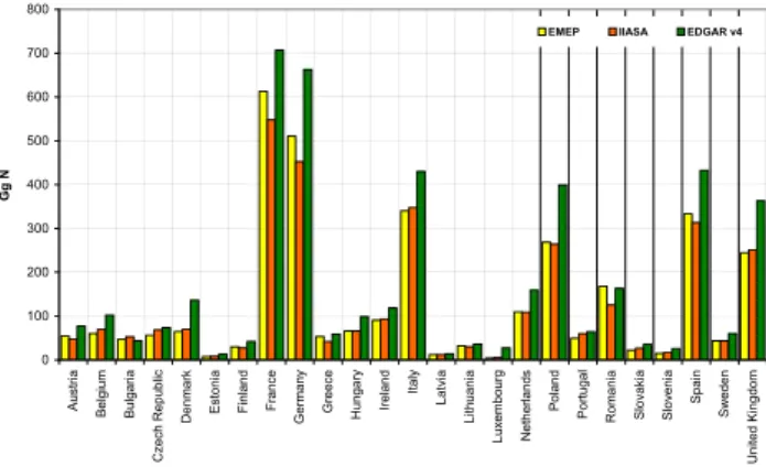
Table 3.Overview over all regional emission inventories used in this paper.
Inventory Substances covered Time scale covered Geographical coverage Spatial disaggregation URL/Reference EMEP NH3, NOx, CO, SO2, NMVOC, PM, Heavy Metals, POPs 1980–2007 (reported) Europe, Russian Federation, Belarus, USA, Canada 50 km×50 km http://www.ceip.at
projections to 2030 (area covering all parties to the CLRTAP) (10 km×10 km planned)
Parties to the Convention on Long-Range Transboundary Air Pollution (CLRTAP) are legally required to report emission data to the European Monitoring and Evaluation Programme (EMEP) on an annual basis. This includes spatially disaggregated data every 5 years (2000, 2005, . . . ) as well as supporting information (activity data, Informative Inventory Report IIR). Theoretically, a full inventory should be available with approx. a two year time lag (e.g. data for 2007 have to be reported in 2009), however, individual parties do not always report on time or fully complete datasets. While the EMEP Centre for Emissions and Projections (CEIP) monitors reporting compliance and supports inventory reviews, datasets for modelling have to be gap-filled frequently to allow for modelling over the full spatial domain, without data gaps.
EDGAR v4 CO2, N2O, CH4, F-Gases, CO, NOx, 2000–2005 Global(Regions/Countries) 0.1◦×0.1◦ http://edgar.jrc.ec.europa.eu NMVOC, NH3, SO2, PM2.5,10, BC, OC, POPs
The EDGAR 4 dataset is thelatest version of a series and is currently maintained and hosted by the Joint Research Centre of the European Commission at Ispra/Italy. With its global coverage, comprehensive set of substances and high spatial resolution, the EDGAR 4 inventory is designed for use as input for global/regional atmospheric and climate models. It is not based on reported emissions, but calculated bottom-up using emission factors (EFs) and estimated activity rates for each source sector.
EDGAR32 FT2000 CO2, CH4, N2O, F-Gases, CO, NMVOC, NOxand SO2 2000 Global(Regions/Countries) 1◦×1◦ http://www.mnp.nl/edgar/model/v32ft2000edgar/
The Fast Track (FT) 2000 dataset has been published in 2005, based on the EDGAR 3.2 estimates for 1995 and prepared by trend analyses at country level for each
standard source category of EDGAR 3.2. Thus, the sectoral structure and other features for EDGAR 3.2 and FT 2000 are the same. As one caveat, NH3emission data
have not been calculated for the year 2000 in either EDGAR 3.2 or FT 2000 and have only been available for 1990 based on GEIA/EDGAR 2.1 data.
EDGAR Hyde 1.3/1.4 CO2, CH4, N2O, CO, NOx, NMVOC, SO2and NH3 1890–1990(10 year time steps) Global(Regions/Countries) 1◦×1◦ http://www.mnp.nl/edgar/model/100 year emissions/edgar-hyde-1.3/
http://www.mnp.nl/edgar/model/100 year emissions/edgar-hyde-1.4/
Based on EDGAR v2 and the History Database of the Global Environment (HYDE) global anthropogenic emissions for the period 1890–1990 by 13 world regions and on 1 x 1 degree grid have been constructed (Van Aardenne et al., 2001). EDGAR Hyde has been developed by the National Institute for Public Health and Environment (RIVM) and Utrecht University, The Netherlands.
UNFCCC CO2, CH4, N2O, PFCs, HFCs, SF6 1990–2006 Global(Parties to the UNFCCC) N/A http://unfccc.int/ghg{ }data/items/3800.php
Parties to the United Nations Convention on Climate Change (UNFCCC) report greenhouse gas (GHG) emissions annually to UNFCCC. The sectoral structure of the Common Reporting Format (CRF) is similar to the NFR used for EMEP reporting, but mainly tailored for fossil fuel combustion sources.
IIASA GAINS SO2, NH3, NOx, VOC, PM (TSP, PM10, PM2.5and PM1), 2000–2030 Europe (EU27 and Central and Eastern European N/A (mapping http://gains.iiasa.ac.at BC, OC, CO2, CH4, N2O, F-Gases Countries), Russian Federation, China, South-Asia, Rest of the World of model output)
The GAINS model has been implemented for the analysis of air pollution control and greenhouse gas mitigation strategies for a number of regions. The online version of GAINS provides access to all input datasets, including emissions in year time steps. For comparing with European inventory datasets, the NEC2007 baseline scenario has been selected.
www
.atmos-chem-ph
ys.net/9/76
57/2009/
Atmos.
Chem.
Ph
ys.,
9,
7657–
7677
,
below the EMEP figures. The reason for this small differ-ence in emissions that have the same underlying data sources is most likely revised animal numbers or more detailed emis-sion calculations that have been available to the experts dur-ing the consultations, but have not yet been used to sub-mit recalculated inventory figures to EMEP. The compari-son with the EDGAR v4 dataset (EDGAR, 2009) shows that EDGAR emissions are (consistently) higher for the bulk of EU27 countries (32%). As a major difference, the EDGAR emissions for agricultural sources are significantly higher than those reported to EMEP, with emissions from agricul-tural soils being most likely the main contributor to the dif-ference observed. A more detailed analysis is not straightfor-ward due the degree of completeness of EMEP emissions re-ported based on the current reporting format (Nomenclature for Reporting, NFR08), which distinguishes in sufficient de-tail emissions within the agricultural sector (currently avail-able for 10 countries). An in-depth assessment is thus con-ducted for the case of the UK in Sect. 6.2.2.
For the European region, including the EU27, the acces-sion countries (Turkey, FYR of Macedonia and Croatia), as well as Norway and Switzerland, the EMEP inventory amounts to 4.5 Tg of NH3for the year 2005 (3.3 Tg N). This
is comparable with an estimate of 4.1 Tg NH3for the whole
of Europe made by Bouwman et al. (1997) for the year 1990 and an estimate of 5.3 Tg NH3(4.3 Tg N) by EDGAR
(2009) for the same set of European countries. Galloway et al. (2004) only give a combined figure for Europe and the former Soviet Union (FSU), with atmospheric emissions of ammonia calculated at 8 Tg N yr−1, with FSU emissions in
1990 at 3.4 Tg N yr−1according to the EDGAR dataset. 2.2 Nitrogen oxides
Nitrogen oxides have been the focus of significant emis-sion control activities in recent decades, both for stationary sources (mainly large combustion plants) and mobile sources (especially road transport). In general it should be antici-pated that NOxemission figures are less uncertain than those
of NH3 or N2O and the initial comparison between EMEP
and EDGAR datasets for 2005 confirms this with only slight differences for individual countries (see Fig. 2). Total NOx
emissions (expressed as NO+NO2) for Europe are estimated
at 11.5 Tg NOx by both EDGAR v4 and EMEP (EDGAR,
2009; EMEP, 2009) for the year 2005 (3.5 Tg N).
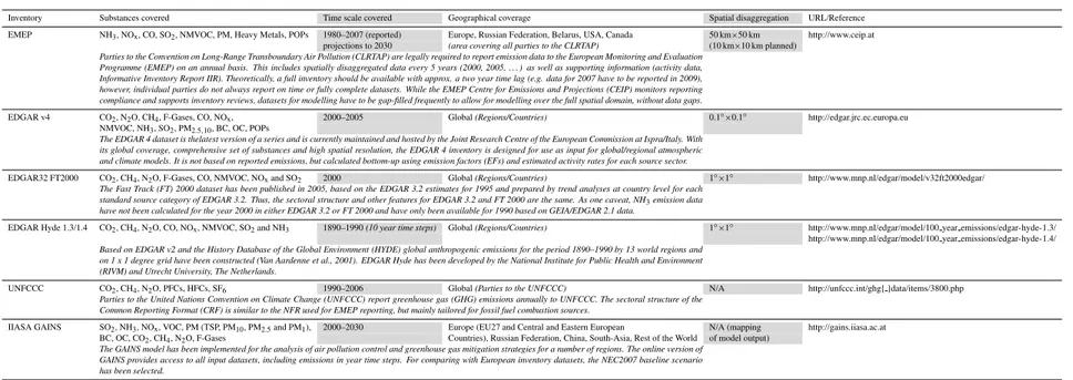
This comparison indicates that NOx emissions are better
understood than for instance NH3, in general. National totals
do not display large variations between inventories; however, sectoral differences can be significant for individual coun-tries. Issues such as an overall lack of measurement pro-grammes, for instance for new vehicle technologies in road transport, and the uncertainties in the effects of decentralised power generation in a liberalised energy market on power plant emissions are likely to have an effect on the quality of NOx inventory datasets also in the future. For an in-depth
0 100 200 300 400 500 600 Au st ri a Belg iu m Bu lg ar ia C z ec h Re pub lic De n m a rk Est o ni a F inl an d Fr a n ce Ge rm a n y Gr ee ce Hun gary Irel an d It a ly La tv ia Lith ua ni a L u x e mb ourg Ne th e rla n d s Po la nd P o rt uga l Roma nia Sl ov a k ia S lov en ia Spa in Sw ede n U n it e d Ki ng do m Gg N
EMEP IIASA EDGAR v4
Fig. 2.Comparison of EU27 (not showing Malta and Cyprus)
emis-sions of NOx(expressed as Gg N) reported to EMEP (EMEP, 2009) and presented in the EDGAR database (EDGAR, 2009) for the year 2005. 0 20 40 60 80 100 120 140 160 180 Au st ri a Be lgi u m B u lga ria Cz ec h R e pub lic De n m ark Eston ia Fi n land Fr an ce Ge rm an y Gr ee ce Hu ng ary Ir el a n d It a ly L a tvia Li th ua ni a Lu xe m b o u rg Ne th e rl a n d s Po la nd Po rtu gal Ro m ania Sl ov ak ia Sl ov e n ia Sp ai n Sw ed en Uni ted Kin gdo m Gg N
UNFCCC IIASA EDGAR v4
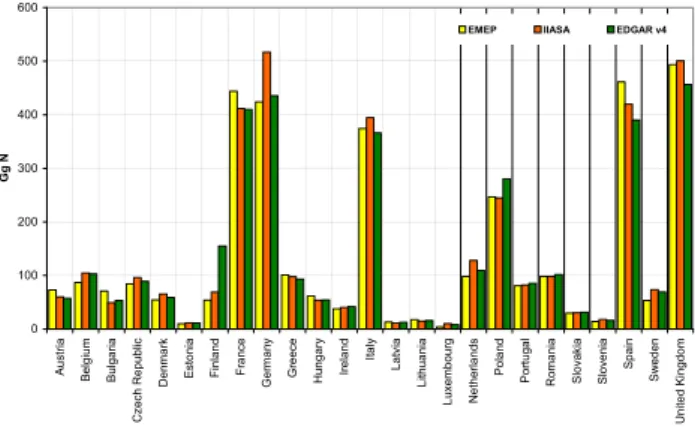
Fig. 3. Comparison of EU27 (not showing Malta and Cyprus)
emissions of N2O (expressed as Gg N) reported to UNFCCC (with-out LULUCF, UNFCCC, 2009) and presented in the EDGAR v4 database (EDGAR, 2009) for the year 2005.
assessment of e.g. sectoral differences between inventories, up-to-date and documented national emission factors based on measurements for different technologies would be vital.
2.3 Nitrous oxide
Since N2O emissions are not reported under the CLRTAP, but
subject to reporting obligations to the UNFCCC for Table 3 countries, the comparison is made between data collected un-der the UNFCCC and the EDGAR v4 inventory (Fig. 3).
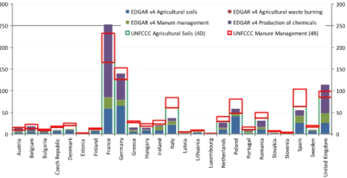
S. Reis et al.: Reactive nitrogen in atmospheric emission inventories 7663 0 50 100 150 200 250 300 Au st ri a Be lg iu m Bu lg ar ia Cz e ch R e p ubl ic De n m ar k Es to n ia Fi n la n d Fr a n ce Ge rm a n y Gr eece H ung a ry Ir el a n d It a ly Lat via Li th u a n ia Lu xem b o u rg Ne the rl a nds Po la n d Po rt u g a l Ro m a n ia Sl ov a ki a Sl o ve n ia Sp a in Sw ed en Un it e d Ki ng do m 0 50 100 150 200 250 300 EDGAR v4 Agricultural soils EDGAR v4 Agricultural waste burning EDGAR v4 Manure management EDGAR v4 Production of chemicals UNFCCC Agricultural Soils (4D) UNFCCC Manure Management (4B)
Fig. 4. Relative contributions of N2O emissions (in Gg N2O)
from agricultural sources soils and manure management in the EU27 countries (not displaying Cyprus and Malta) according to the EDGAR v4 inventory (EDGAR, 2009) and compared to major agri-cultural sources as reported to UNFCC (Agriagri-cultural Soils, NRF 4D; Manure Management, NRF 4B) (UNFCCC, 2009).
the uncertainty in either dataset, but it should be stated that recent findings of Skiba et al. (2001) provide a methodol-ogy for the calculation of N2O emissions from soils, one of
the main sources of N2O, which results in higher emissions
than the current UNFCCC established methodology. Within the EU27, 48% of N2O emissions in the EDGAR v4
inven-tory stem from agricultural sources (34.2% from agricultural soils, 13.9% from manure management and 0.1% from agri-cultural waste burning). Shares of emissions from agricul-tural soils in individual countries vary significantly, between 9.6% (Greece) and 67.6% (Denmark). Figure 4 highlights the variation of relative contributions of agricultural soils and manure management to N2O emissions in the EU27
coun-tries for a comparison between EDGAR v4 and UNFCCC. A third contributing source to N2O emissions in the EU27 is
the chemical industry sector, contributing about 28% of to-tal N2O emissions in 2005 in EDGAR v4. It is likely that
emissions from the chemical industry are well understood and hence emission factors and activity rates can be assumed to be less uncertain than those from agricultural soils or ma-nure management. Hence, the differences between UNFCCC and EDGAR data most likely mainly arise from the applica-tion of different emission factors (or activity rates) in these two sectors.
Figure 4 illustrates the difference between the main sources of N2O emissions with a focus on emissions from
agricultural sources. There is a clear indication that emis-sions reported to UNFCCC under CRF (Common Reporting Format) categories 4B (Manure Management) and 4D (Agri-cultural Soils) are substantially higher than those estimated in EDGAR v4 under the same headings.
However, even in those cases were both inventories pro-vide similar figures, a more thorough investigation of emis-sions from agricultural soils may be required in the light of the findings of Skiba et al. (2001), Crutzen et al. (2008) and Mosier et al (1998), which indicate a potential
underestima-tion of N2O emissions from soils in current inventories. The
increasing demand for bio fuels could even lead to a larger underestimation, unless future emission factors take these findings into account.
3 Emission inventories of reactive nitrogen species in the United States of America
The US Environmental Protection Agency is charged with developing the National Emission Inventory (NEI, US EPA, 2009a) in support of the Clean Air Act and subsequent amendments. The NEI includes an accounting of pollutants that impact air quality, including NOx and NH3. These
ef-forts have recently been reviewed in an assessment report by NARSTO (2005). In addition, the EPA prepares an estimate of N2O emissions in the US Inventory of Greenhouse Gas
Emissions and Sinks (US EPA, 2009b), in accordance with the UNFCCC.
3.1 Ammonia
The NEI estimates that more than 80% of total USA ammo-nia emissions are from livestock manure management and application of chemical fertilizers. The next largest source is ammonia from vehicles equipped with catalytic converters, which comprises approximately 7% of the inventory. While the NEI and EDGAR database have similar total agricultural and vehicle emissions, 14% of the EDGAR NH3emissions
are from industrial combustion, while this source is less than 1% in the NEI.
Because of the operational challenges in measuring am-monia emissions and a lack of detailed animal husbandry practices data, ammonia emission estimates have high uncer-tainty. Independent efforts to quantify the seasonal variabil-ity have shown agreement for winter and summer emissions, but differ for the spring and fall (Gilliland et al., 2006: Pinder et al., 2006: Henze et al., 2008). Because atmospheric agri-cultural emissions are rarely regulated, the trend in emissions is expected to be proportional to the increase in livestock population and acres under cultivation. Both are expected to increase in coming years (USDA, 2007).
3.2 Nitrogen oxides
The NEI estimates that the largest contributors of US NOx
emissions include on-road vehicles (32%), off-road vehi-cles (30%), such as ships, aircraft, and construction equip-ment, and electricity and industrial power generation (27%). Emissions from on-road and off-road vehicles are calcu-lated using the National Mobile Inventory Model (NMIM) (http://www.epa.gov/otaq/nmim.htm). While not used in this study, a more advanced mobile source emissions model, MOVES (http://www.epa.gov/otaq/models/moves/), is cur-rently under development and a draft version is available for public use. Important improvements include more detailed
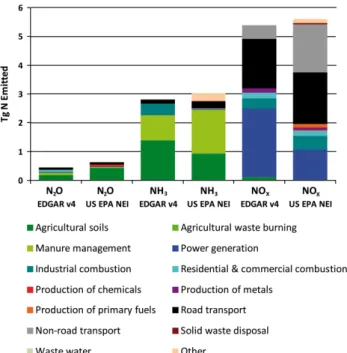
Fig. 5.Comparison of US EPA emissions of N2O, NH3, and NOx with the EDGAR database for the year 2005 (USEPA, 2009a, b; EDGAR, 2009).
inspection and maintenance data and better representation of extended idling emissions.
Despite increased diesel and gasoline consumption, NOx
emissions from on-road sources are estimated to have de-creased by on average 5% per year since 2002 due to the introduction of stricter emission standards. Parrish (2006) used ambient data to show that total on-road emissions may have increased from 1990–2000; however, in a multi-city, multi-year study, Bishop and Stedman (2008) have demon-strated that per-car emission factors have decreased from 2000 to 2006. The NEI reports little year-to-year change in off-road vehicle emissions. Many electricity and industrial power generation facilities have been subject to several re-cent regulated emission reductions including the NOx
Bud-get Trading Program. Because most of these facilities are equipped with Continuous Emission Monitors, the emission magnitude and trend is well quantified. Since 1999, this sec-tor has reduced emissions by an average of 6.4% per year. The combined effect of the reductions in mobile and station-ary source NOxemissions has been observed in the surface
concentration monitoring data (Godowitch et al., 2008) and from space-based remote sensing methods (Kim et al., 2006; Kim et al., 2009).
In Fig. 5, EDGAR v4 and US EPA NOx emission data
are aggregated by sector to make them directly compara-ble. Where stationary combustion sources are concerned, EDGAR has markedly larger emissions. The NEI power gen-eration emission rates are likely more accurate since they are measured at the electricity generating units as part of
the Continuous Emission Monitoring System. Road trans-port emissions are similar in both datasets, but interestingly non-road mobile sources (which include off-road vehicles, rail, air and shipping) are significantly larger in the US EPA dataset. The NEI partially includes international shipping emissions near the US coast, which have been omitted from the EDGAR inventory and have been estimated in EDGAR FT32 at about 0.43 Tg N for the US in the year 2000. Another possible explanation is a difference in activity rates and/or emission factors for domestic air transport. From 2000 to 2005, the trends in these two databases also differ. For on-road sources, EDGAR estimates 6% yr−1 reduction (NEI: 4% yr−1), but for power generation and industrial sources, the EDGAR inventory has little trend (NEI: 6% yr−1 reduc-tion).
3.3 Nitrous oxide
Total US N2O emissions for 2005 are estimated to be
1.02 Tg N2O (US EPA, 2009b). The largest source of US
N2O emissions is agricultural soils (67%), followed by
fos-sil fuel combustion in vehicles (12%), industrial processes (8%), fossil fuel combustion for electricity generation (5%) and livestock manure management (4%). Enhancements of N2O emissions from agricultural soils include practices such
as fertilization, application of livestock manure, grazing ani-mals on pasture or feedlots, and cultivation of N-fixing crops. The estimated trend in N2O emissions for the USA is a
grad-ual reduction of approximately 1% per year since 2000. This is due to a 5% reduction per year in the emissions from vehi-cles and industrial processes – the other sectors are estimated to have largely remained constant over this period. EDGAR v4 emissions are lower than those reported by EPA. This is almost entirely due to lower emissions from agricultural soils in the EDGAR v4 inventory.
The physical and chemical processes that drive emissions of NH3, NOx, and N2O are often intertwined. This is also
true for the human activities that cause these emissions, such as fuel combustion in motor vehicles and agricultural land under cultivation. However, the GHG emission inventory and the NEI do not always use the same models and data sources. For example, direct fertilized crop emissions of N2O are
esti-mated using the DAYCENT model (Del Grosso et al., 2001), while the temporal pattern of NH3 emissions are estimated
S. Reis et al.: Reactive nitrogen in atmospheric emission inventories 7665
0 2 4 6 8 10 12 14
NH3 NOx N2O (x10)
Tg
N
Waste water
Solid waste disposal
Non‐road transport
Road transport
Industrial production processes
Manufacturing industry
Residential
Fuel production/transmission
Energy industry
Manure management
Agricultural waste burning
Agricultural Soils
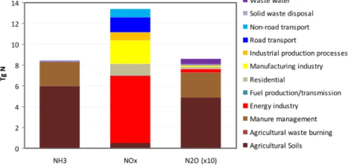
Fig. 6. Emissions of NH3, NOxand N2O (expressed in Tg N) for the China in 2005 according to the EDGAR v4 inventory (EDGAR, 2009) for the main emitting source sectors. N2O emissions are in-creased by a factor of 10 for ease of comparison.
4 Emission inventories of reactive nitrogen species in China
The analysis of the emission situation in China is compara-tively more difficult than is the case for Europe or the United States. Reasons for this are, among others, the immense growth rates of the economy and thus fast developing emis-sion sources, the lack of an official national inventory pro-gramme and no reporting of emissions to international organ-isations. Figure 6 displays the emission estimates for the year 2005, distinguishing the main source sectors. NH3and N2O
emissions are here dominated by agricultural sources (mainly agricultural soils and manure management), while for NOx,
the main difference to Europe and the US is the large share of stationary combustion relative to mobile sources. In the following sections, recent studies are discussed for each of the substances.
4.1 Ammonia
Only a few studies on ammonia emissions in China are avail-able (e.g. Zhao et al., 1994; Yan et al., 2003). With regard to total NH3emissions in China, the major contribution comes
from N-fertilizer application (52%) and livestock (41%) re-spectively in the 1990’s (Klimont, 2001a). Other sources of ammonia emissions include biomass burning, natural ecosys-tems, crops and oceans, humans (breath, sweat, excretion) and fossil fuel combustion.
The basic methodology applied to derive these emissions relies on the approach used in Europe (Klaassen, 1994; Klimont, 2001b), and as far as available takes into account information about China-specific characteristics. Klimont (2001a) estimated the total ammonia emissions in China at 9.7 Tg NH3in 1990 (11.7 Tg NH3in 1995), which translates
into 7.98 Tg N (1990) respectively 9.62 Tg N (1995). Emis-sions were as well spatially disaggregated on a 1◦×1◦grid for both years. In 1995 the highest ammonia emission den-sity, exceeding 100 Gg NH3per grid, is observed inJiangsu
andHenanprovinces. This corresponds well with the large population of pigs in these regions as well as high cattle density inHenanprovince. Using the IPCC approach, NH3
emission from synthetic fertilizer and manure application in 1990 was estimated to be 1.65 Tg N by Li Yu’e et al. (2000). Yan et al. (2003) quantified the use of urea and ammonium bicarbonate and the cultivation of rice leading to a high av-erage ammonia loss rate from chemical N fertilizer in East, Southeast and South Asia, and the total emission was esti-mated to be 5.8 Tg N for the area of China. These values compare reasonably well with the amount of 8.4 Tg N from NH3 emissions for China in EDGAR v4, with 6.01 Tg N
(72%) stemming from agricultural soils and 2.29 Tg N (27%) from manure management.
Due to anticipated increases in synthetic fertilizer applica-tion rates and per-capita meat and dairy consumpapplica-tion, future ammonia emissions are expected to continue to rise.
4.2 Nitrogen oxides
East Asia is a region of the world with large and rapidly increasing anthropogenic emissions, NOx emissions have
increased by 58% from 1975 (2.05 Tg N yr−1) to 1987 (3.25 Tg N yr−1) (Kato and Akimoto, 1992), and Van Aar-denne et al. (1999) anticipated an almost fourfold increase in NOxemissions for the period from 1999 to 2020. Especially
in China, anthropogenic emissions associated with fossil fuel combustion have grown significantly due to a period of rapid economic development and industrial expansion in the last three decades (e.g., Streets and Waldhoff, 2000).
Using data from the China Statistical Yearbook (Press, 1996), Akimoto et al. (1994) and Kato and Akimoto (1992) estimated NOx emissions in China for the year 1987. Bai
(1996) considered that the inventory should be based on more detailed data than available from the Yearbook, and the emis-sion factors should be modified to be consistent with ac-tual emission factors applicable to the situation in China. Bai (1996) provided a NOx emission inventory for the year
1992 using more detailed data from statistical yearbooks on a provincial level and emission factors measured in Chinese installations.
Bai (1996) created a spatially disaggregated inventory on 1◦×1◦ with the highest grid value being >0.1 Tg N yr−1, which occurred only in Shanghai. From the east to the west of China, the values decreased. The emissions in some provinces such as Inner Mongolia, Qinghai and Tibet are even<0.0001 Tg N yr−1, which is consistent with the dis-tribution of industrial installations and population between these regions.
The rapid growth of NOxemissions in China (Bai, 1996;
Ma and Zhou, 2000; Streets et al., 2000), with an increase from 9.5 Tg to 12.0 Tg (calculated as NO2) between 1990
and 1995 is driven by a significant increase in emissions from the transport sector (increase of 62%). Emissions also in-crease significantly in the industrial, power generation and
domestic sectors, with increases of 26%, 20% and 21%, re-spectively. Within these sectors, emissions from industrial installations were the largest individual source group, con-tributing approx. 42% of total emissions (5.0 Tg NOx as
NO2). From 1995 to 2000, some studies (e.g., Aardenne
et al., 1999; Streets et al., 2000) estimated that NOx
emis-sions in China will continue to grow rapidly. However, other researches’ results using more recent statistical data (e.g., Tian et al., 2001) indicate that NOx emissions began to
re-main somewhat stable for a few years with total emissions in China amounting to 11.3 Tg NOx(as NO2) in 1995, 12.0 Tg
(1996), 11.7 Tg (1997) and 11.2 Tg (1998). In the analy-sis by Tian et al., this is explained on the baanaly-sis of chang-ing energy management in China. However, for the same time period (1995-2000), Ohara (2007) and IIASA (2009) estimated a slow increase of emissions from 9.31 Tg NOx
to 11.19 Tg NOx(Ohara, 2007), respectively 9.38 Tg NOxto
11.73 Tg NOx(IIASA, 2009), all calculated as NO2(see as
well Fig. 9 for the development over the whole period). According to Streets et al. (2003) Chinese emissions in the year 2000 have only slightly increased (11.3 Tg NOx).
For the year 2005, however, both EDGAR (2009) and IIASA (2009) estimate further increases to 18.35 Tg NOx(as NO2)
and 17.09 Tg NOx(as NO2) respectively. Based on EDGAR
(2009), power generation still contributes the lion’s share of NOxemissions in China (48%), while road transport is still
comparatively low at 11%. In addition to that, satellite ob-servations of the tropospheric NO2column density over
East-ern China have increased considerably during 1996 to 2004 (Richter et al., 2005; van der A et al., 2006), suggesting large emission increases over that period
4.3 Nitrous Oxide
The UNDP/GEF ECPINC Project (Enabling China to Prepare Its Initial National Communication, http://www. ccchina.gov.cn/en/NewsInfo.asp?NewsId=5392) has been implemented to support China in fulfilling its commitments under the UNFCCC to communicate to the Conference of Parties to the Convention (1) a national inventory of emis-sions and sinks of greenhouse gases (2) a general descrip-tion of steps taken or envisaged by China to implement the Convention and (3) any other information China considers relevant and suitable for inclusion in its Communication.
A fair amount of research has been conducted on an N2O
emissions inventory for China. Zheng et al. (2004) have shown that most (up to 75%) of cropland N2O emissions are
direct emissions: immediately from fertilized top-soil rather than denitrification of nitrate leached into sub-surface and groundwater. Zheng et al. (2004) collected 54 direct N2O
emission factors (EF′ds) obtained from 12 sites of Chinese
croplands and found that of these 60% are underestimated by 29% and 30% are overestimated by 50% due to observa-tion shortages. The biases of EFds are corrected and their
uncertainties are re-estimated. Of the 31 site-scale EFds,
42% are lower by 58% and 26% are higher by 143% than the IPCC default values. Periodically wetting/drying the fields or doubling nitrogen fertilizers may double or even triple an EFd. The direct N2O emissions from Chinese
crop-lands are estimated at 275 Gg N2O-N yr|1 in the 1990s, of
which 20% is due to vegetable cultivation. The great uncer-tainty of this estimate, −79% to 135%, is overwhelmingly due to the huge uncertainty in estimating EFds (−78±15%
to 129±62%). The direct N2O emission intensities
signif-icantly depend upon the economic situation of the region, implying a larger potential emission in the future.
However, agricultural activity is the main, but not the only source of N2O emissions in China. According to results
by Li Yu’e et al. (2000), total N2O emissions from
station-ary fuel combustion amounted to 58.22 Gg N yr−1in 1990 in
China. Within the fuel combustion sector, energy industries, manufacturing industries and residential areas were the main sources of N2O. Among fossil fuels, hard coal was the main
contributor to N2O emissions. The industrial process sector
was a less critical source of N2O emissions, with the total
N2O emissions from this source group amounting to 0.41–
0.90 Gg N yr−1. The total emission of N2O as a result of
fertilizer application was 342.5 Gg N yr−1in 1990, being the most important contributor to N2O emission from
agricul-tural soils.
While both Li (2000) and Xing’s (1998) estimations did not consider permanent croplands, Lu et al (2006) estab-lished an empirical model to develop a spatial inventory at the 10×10 km scale of direct N2O emissions from
agri-culture in China, in which both emission factor and back-ground emission for N2O were adjusted for precipitation.
As a result, the total annual fertilizer-induced N2O emission
was estimated to be 198.89 Gg N2O-N in 1997 and
back-ground emissions of N2O from agriculture was estimated
to be 92.7 Gg N2O-N and the annual N2O emission totalled
291.67 Gg N2O-N. All N2O emission measurements are
sub-ject to significant uncertainty due to their great temporal and spatial variations of cropland fluxes.
For the years 2000 and 2005, EDGAR (2009) esti-mates 928 Gg N2O (2000) and 1065 Gg N2O (2000). This
is consistently lower than figures by IIASA (2009), with 1,747 Gg N2O (2000) and 1,854 Gg N2O respectively. It has
to be noted, that EDGAR 32 FT 2000 had estimated N2O
emissions for China at 1764 Gg N2O, which is comparable
S. Reis et al.: Reactive nitrogen in atmospheric emission inventories 7667
5 Evaluation of emission inventories for reactive nitro-gen
5.1 Uncertainty assessment in general
For all emission inventories portrayed here, the assessment of uncertainties is a key aspect. For national inventories, is-sues of compliance or non-compliance with reduction targets and emission ceilings are relevant, while in general the quan-tification of uncertainties of emissions as input data for atmo-spheric dispersion models is of importance. Aspects of com-pleteness regarding the total amount of emissions accounted for are as important as the spatial distribution, chemical com-position and temporal patterns of emission occurrences.
Within the context of emission inventories compiled un-der the CLRTAP, country submissions are accompanied by so-called informative inventory reports (IIRs, http://www. emep.int/emis2007/reportinginstructions.html), covering as-pects of completeness, an analysis of key sources and uncer-tainties. In addition to this, regular centralised reviews are conducted for selected countries, with the aim to improve the quality and accuracy of reported emission data. For the United States, NARSTO’s third assessment reportImproving Emission Inventories for Effective Air Quality Management Across North America: A NARSTO Assessment(NARSTO, 2005) took stock of the current state of emission inventories for Canada, the United States and Mexico and identified ar-eas for improvement.
Under the UNFCCC, emission reporting is guided by a document called “Good Practice Guidance and Uncertainty Management in National Greenhouse Gas Inventories” (http: //www.ipcc-nggip.iges.or.jp/public/gp/english/, see as well IPCC 1997, 2000) in order to“...to assist countries in pro-ducing inventories that are neither over nor underestimates so far as can be judged, and in which uncertainties are re-duced as far as practicable.”
These formalised assessments of inventories are relevant sources of information when trying to identify the overall ac-curacy of emission estimates, for instance, on a national scale or across countries for individual pollutants. In addition, studies such as conducted by Winiwarter and Rypdal (2001) and Rypdal and Winiwarter (2001) provide a methodologi-cal analysis of uncertainties for specific trace gases, respec-tively individual countries. An analysis conducted by Olivier et al. (1999) discusses in detail uncertainties of GHG emis-sions on a sector level, distinguishing between uncertainties in activity datasets, emission factors (as the main drivers of uncertainties in inventories) and the resulting total emissions. Olivier et al. (1999) conclude that emissions from fossil fuel production and combustion are generally well under-stood and prone to small to medium uncertainties only. This can be said as well for industrial production processes or sol-vent use. In contrast, emissions related to agricultural land-use are viewed as significantly more uncertain. In a simi-lar way, emission estimates of N2O and CH4are generally
less robust, because CO2 is emitted from combustion
pro-cesses mainly can be calculated more accurately than emis-sions based on soil microbial processes for instance. These findings have implications as well for the discussion of the different substances in the inventories analysed in this paper, where NOxemissions can be seen comparatively robust. Yet,
the uncertainty associated with NOxemissions is approx. 4
times higher than for CO2 emissions, because these are
di-rectly linear to fuel input in combustion sources and EFs are not influenced by processes and hence easier to determine. On the other hand, NH3 and even more so, N2O emissions
are likely to be more uncertain because their main sources are related to agriculture and affected e.g. by soil biochemi-cal processes and meteorologibiochemi-cal and climatologibiochemi-cal drivers. For individual inventories, e.g. the UK NAEI, un-certainty assessments are provided by inventory compil-ers (http://www.naei.org.uk/emissions/emissions 2007.php? action=notes1). For NOx, the NAEI assumes ±7%, for
NH3±20%, while for N2O no individual assessment is made,
but an overall uncertainty of±15% is estimated across the 6 greenhouse gases overall.
Following the differences in sectoral uncertainties pro-vided by Olivier et al. (1999), the following sections will specifically investigate differences in sectoral emissions be-tween inventories in order to identify, if current inventory differences are within range of the uncertainty estimates.
5.2 Inventory comparison – analysing differences and similarities
5.2.1 General observations for the situation in Europe
A full and detailed intercomparison of the inventories on the most detailed sectoral level for all countries/regions is be-yond the scope of this paper. However, some similarities and differences are worth noting. In the case of ammonia, both the EMEP and the IIASA figures are quite similar, with some countries showing different emission levels, most likely due to recalculations and re-assessments of e.g. animal numbers that have been emerging in the course of bilateral consulta-tions in the preparation of the IIASA dataset and which have not (yet) been incorporated in recalculations of the data re-ported to EMEP.
With regard to NOx, the differences between EMEP and
EDGAR figures are substantial for some countries and re-markably different in total (EDGAR v4 32% higher than EMEP). Some of the potential sources of these discrepancies have been highlighted in Sect. 3.3, in particular the different sectoral allocations including some emission sources that are not reported under EMEP in the EDGAR dataset.
In addition to that, a likely reason for these large differ-ences are assumptions regarding underlying emission factors for some of the largest contributing sources, e.g. due to the estimated share of power plants equipped with efficient NOx
0% 10% 20% 30% 40% 50% 60% 70% 80% 90% 100%
EMEP 2005 NH3 EMEP 2005 NOx
R_Other Q_Agriculture ‐ wastes P_Agriculture ‐ other O_Agriculture ‐ livestock N_Waste incineration M_Waste water L_Other waste disposal K_International LTO J_Domestic LTO I_Off‐Road mobile sources H_Shipping
G_Road & rail transport F_Solvent use E_Fugitive fuel emissions D_Industrial processes C_Small combustion B_Industrial combustion A_Public power
0% 10% 20% 30% 40% 50% 60% 70% 80% 90% 100%
EDGAR v4 NH3 EDGAR v4 NOx
Waste Management
Manure Management
Agricultural waste burning
Agricultural soils
Non‐road transport
Road transport
Production of non‐metallic minerals
Production of non‐ferrous metals
Production of iron and steel
Production of chemicals
Fuel production/ transmission
Residential
Manufacturing industry
Energy industry
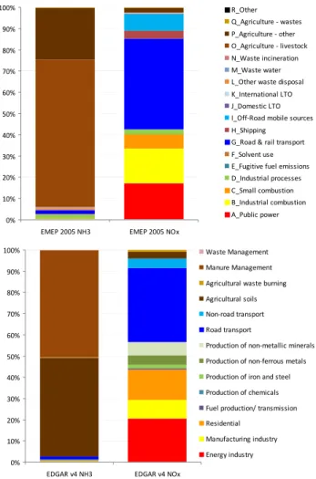
Fig. 7.Sectoral comparison of emissions for the year 2005 between EMEP (top; EMEP, 2009) and EDGAR v4 (bottom; EDGAR, 2009) for the EU27 countries (excluding Malta and Cyprus). It should be noted, that the EMEP sectoral split is based on only 10 countries reporting according to the latest sectoral structure (NFR 08, Level 1), which is best comparable with the EDGAR v4 sector structure.
control equipment, or emission factors and activity rates for road transport sources.
Figure 7 displays a direct comparison of NH3 and NOx
emissions in the EMEP and the EDGAR v4 inventories by sector for the year 2005. The most recent change in EMEP reporting requirements, adopting a new reporting format termed NFR 08 (Nomenclature for Reporting 2008) which is – even on an aggregated level – better suited for sectoral analysis than its predecessors (e.g. NFR 01, NFR 02) which were based on the UNFCCC CRF format and in some ar-eas lacking a sufficient level of detail. With regard to NH3,
agricultural emissions show a similar pattern in both invento-ries overall and are dominating emissions for this substance. The situation for NOxemissions is more diverse and shows a
distinct difference for stationary combustion sources, which contribute more than 55% to EDGAR v4 NOxemissions, but
only account for about 42% of EMEP NOxemissions. A full
comparison of individual sectors by country on a European scale would be worthwhile once all countries are reporting emissions based on the new NFR 08 sectoral structure. As this is not feasible at this stage and within the scope of this paper, an analysis is conducted for the United Kingdom in the following section.
5.2.2 Detailed analysis for the United Kingdom
For a thorough investigation of the differences between in-ventories, it is essential to have access to a very detailed sectoral split, and if feasible, even the emission factors and activity rates that have been used to compile the invento-ries. In this context, the structure initially applied in the EMEP inventories labelled SNAP (Selected Nomenclature for Air Pollution, EMEP) provided emission data with a de-tailed level 3 split allowed for a comparison down to pro-cess and fuel level. However, not many countries provided the obligatory information in this detailed split and hence in-ventories were subject to different levels of detail and sub-stantial gaps. The new format for reporting under EMEP has been termed Nomenclature for Reporting (NFR, current version is NFR 08). While NFR has been closely aligned with the UNFCCC common reporting format (CRF) and thus been mainly driven by fossil fuel combustion sources, it provided less detail and no distinctions had been made for instance with regard to the type of fuel used in power plants or road transport modes. The recently adopted NFR 08 better accounts for non-combustion sources and already on the most aggregated level (NFR 08, Level 1) provides a useful split into the main sectors (for details on NFR 08, see http://www.unece.org/env/documents/2008/EB/EB/ ece.eb.air.2008.4.e.pdf). The sectoral split used in EDGAR v4 reflects the bottom-up character of the inventory. It is not always directly comparable to NFR sectors, but in most cases, an equivalent source sector allocation – on a more ag-gregate level – can be found.
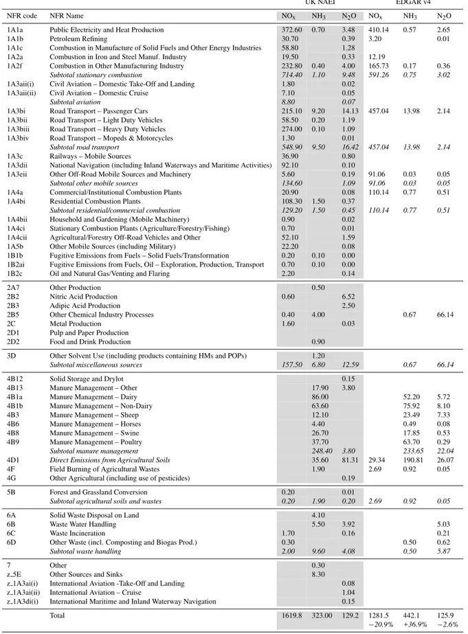
Table 4 provides a detailed comparison of source sectors split into categories for which a cross-comparison between the UK NAEI and EDGAR v4 could be sensibly conducted for NOx, NH3and N2O. As some of the individual source
sectors in NAEI and EDGAR do not fully match, the follow-ing discussion will focus on the subtotals for sector groups rather than on individual figures.
The figures for stationary combustion are quite similar overall, but NOx emissions in EDGAR v4 are 17% lower,
N2O from this source group is less than a third than those
in the NAEI. For road transport, the picture is similar (17% lower NOx emissions, 87% lower N2O emissions), while
NH3 from road transport is 47% higher in EDGAR v4.
NOx emissions from other mobile sources and machinery
S. Reis et al.: Reactive nitrogen in atmospheric emission inventories 7669 differences in these sectors between NAEI and EDGAR v4,
however, is larger than anticipated taking into account the uncertainty ranges assumed for the UK NAEI (see section 6.1).
On the other hand, total NH3 emissions from the
sec-tor manure management are quite similar (∼6% lower in EDGAR v4), yet some significant differences between the emissions from individual animal types can be observed. EDGAR v4 has substantially higher emissions of N2O from
manure management (about 6 times higher than NAEI), but less than one third of direct emissions from agricultural soils. This may hint at a difference in allocation between these sub-sectors. In addition to that, NH3emissions directly
originat-ing from agricultural soils are 5.3 times higher in EDGAR v4.
Finally, NAEI lists a few sectors that are not subject to reporting obligations under EMEP, while EDGAR v4 – as an inventory primarily compiled for modelling purposes – does not make this distinction.
In summary, the difference between country total emis-sions between both inventories is within the uncertainty mar-gins expected for N2O at 2.6% (±15% uncertainty range for
NAEI, see section 6.1), however larger for NOx emissions
with EDGAR v4 being 20.9% below NAEI, (NAEI assum-ing a±7% uncertainty range). NH3 emissions in EDGAR
v4 are 36.9% higher than in the NAEI (uncertainty range for NAEI assumed to be (±20%). However, for all three sub-stances, sectoral allocation are quite different between in-ventories, which has direct implications for the use of the emissions for atmospheric modelling, e.g. the temporal pro-files and spatial distribution of emissions in different sectors. The current structure of the inventories such as NAEI and hence EMEP – which are compiled primarily for reporting and compliance monitoring purposes – is not always detailed enough for modellers to fully assess the quality of the in-ventory and supporting datasets are often not accessible or documented well enough.
5.2.3 Observations for all regions
The overview comparisons of sectoral emission shares in the US and the China (see Figs. 5 and 6) indicate some substan-tial differences between the emission profiles of the US (and similarly Europe) on one side and China on the other. In particular the high contribution of emissions from agricul-ture to total NH3emissions in general is evident. In the case
of NOx emissions, mobile sources (road transport and
off-road) contribute a larger share in Europe and the US, while power generation based on fossil fuels (coal mainly) in the energy industries of China and the US contribute in a sim-ilar magnitude. A remarkable difference can be seen in the contribution of road transport to N2O emissions and – to a
smaller extent – NH3emissions in the US compared to
Eu-rope. The reason for the difference in transport N2O
emis-sions can be explained by comparing EFs for running (hot)
2 4 6 8 10 12
19
90
19
91
19
92
19
93
19
94
19
95
19
96
199
7
19
9
8
19
99
20
0
0
20
01
20
02
20
03
20
04
20
05
Tg
NH
3
Europe (EDGAR, 2009) Europe (EMEP, 2008)
PR China, (EDGAR, 2009) PR China, (Klimont et al., 2001a)
PR China (EDGAR, 2009) USA (EDGAR, 2009) USA (USEPA, 2006) USA (EDGAR, 2009)
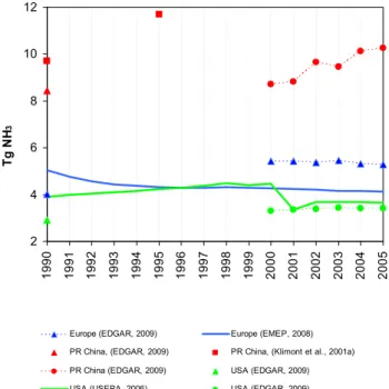
Fig. 8. Estimated trends in NH3emissions in Europe, the US and the China for the period 1990–2005.
emissions for passenger cards advanced three-way catalytic converters) for US and European vehicles in the IPCC Emis-sion Factor Database (EFDB, http://www.ipcc-nggip.iges.or. jp/EFDB/main.php). While the EF for US vehicles is given as 9 mg/km, the EFs for European vehicles (based on the COPRT IV model, http://lat.eng.auth.gr/copert/) range from 0.7 mg/km (highway driving) to 2 mg/km (urban driving). It is not straightforward to assess, if all N2O emissions from
road transport in the US and in Europe have been calculated using these factors, but the magnitude of difference suggests substantially different assumptions as to technology and re-sulting emission factors in both regions.
A comparison between the US NEI and EDGAR v4 in-dicates overall quite similar total figures, except for N2O
(EDGAR v4 substantially higher than US NEI). However, the sectoral structure for NOx and NH3 shows remarkable
difference, for instance regarding the split between manure management and agricultural soils (NH3) and power
genera-tion (NOx).
5.3 Emission trends and implications
Apart from the analysis of emission inventories for specific years, which give a snapshot for a certain point in time, look-ing at the temporal trends in emissions can give valuable in-sight in the development of both emissions as well as the methodologies applied for their calculation.
The trend for NH3 emissions (Fig. 8) shows no
signifi-cant reductions in the 15 year period indicated. A moderate downward trend can be observed in Europe (−18%), which
Table 4.Detailed comparison between source sectors in the UK National Atmospheric Emissions Inventory (NAEI, 2008) and EDGAR v4 (EDGAR, 2009) for the year 2005.
UK NAEI EDGAR v4
NFR code NFR Name NOx NH3 N2O NOx NH3 N2O
1A1a Public Electricity and Heat Production 372.60 0.70 3.48 410.14 0.57 2.65
1A1b Petroleum Refining 30.70 0.39 3.20 0.01
1A1c Combustion in Manufacture of Solid Fuels and Other Energy Industries 58.80 1.28
1A2a Combustion in Iron and Steel Manuf. Industry 19.50 0.33 12.19
1A2f Combustion in Other Manufacturing Industry 232.80 0.40 4.00 165.73 0.17 0.36
Subtotal stationary combustion 714.40 1.10 9.48 591.26 0.75 3.02
1A3aii(i) Civil Aviation – Domestic Take-Off and Landing 1.80 0.02
1A3aii(ii) Civil Aviation – Domestic Cruise 7.10 0.05
Subtotal aviation 8.80 0.07
1A3bi Road Transport – Passenger Cars 215.10 9.20 14.13 457.04 13.98 2.14
1A3bii Road Transport – Light Duty Vehicles 58.50 0.20 1.19
1A3biii Road Transport – Heavy Duty Vehicles 274.00 0.10 1.09
1A3biv Road Transport – Mopeds & Motorcycles 1.30 0.01
Subtotal road transport 548.90 9.50 16.42 457.04 13.98 2.14
1A3c Railways – Mobile Sources 36.90 0.80
1A3dii National Navigation (including Inland Waterways and Maritime Activities) 92.10 0.10
1A3eii Other Off-Road Mobile Sources and Machinery 5.60 0.19 91.06 0.03 0.05
Subtotal other mobile sources 134.60 1.09 91.06 0.03 0.05
1A4a Commercial/Institutional Combustion Plants 20.90 0.08 110.14 0.77 0.51
1A4bi Residential Combustion Plants 108.30 1.50 0.37
Subtotal residential/commercial combustion 129.20 1.50 0.45 110.14 0.77 0.51
1A4bii Household and Gardening (Mobile Machinery) 0.90 0.02
1A4ci Stationary Combustion Plants (Agriculture/Forestry/Fishing) 0.70 0.01
1A4cii Agricultural/Forestry Off-Road Vehicles and Other 52.10 1.59
1A5b Other Mobile Sources (including Military) 22.20 0.08
1B1b Fugitive Emissions from Fuels – Solid Fuels/Transformation 0.20 0.10 0.00
1B2ai Fugitive Emissions from Fuels, Oil – Exploration, Production, Transport 0.70 0.10 0.00
1B2c Oil and Natural Gas/Venting and Flaring 2.20 0.14
2A7 Other Production 0.50
2B2 Nitric Acid Production 0.60 6.52
2B3 Adipic Acid Production 2.50
2B5 Other Chemical Industry Processes 0.40 4.00 0.67 66.14
2C Metal Production 1.60 0.03
2D1 Pulp and Paper Production
2D2 Food and Drink Production 0.90
3D Other Solvent Use (including products containing HMs and POPs) 1.20
Subtotal miscellaneous sources 157.50 6.80 12.59 0.67 66.14
4B12 Solid Storage and Drylot 0.15
4B13 Manure Management – Other 17.90 3.80
4B1a Manure Management – Dairy 86.00 52.20 5.72
4B1b Manure Management – Non-Dairy 63.60 75.92 8.10
4B3 Manure Management – Sheep 12.10 23.49 7.33
4B6 Manure Management – Horses 4.40 0.49 0.08
4B8 Manure Management – Swine 26.70 17.85 0.53
4B9 Manure Management – Poultry 37.70 63.70 0.29
Subtotal manure management 248.40 3.80 233.65 22.04
4D1 Direct Emissions from Agricultural Soils 35.60 81.31 29.34 190.81 26.07
4F Field Burning of Agricultural Wastes 1.90 2.69 0.92 0.05
4G Other Agricultural (including use of pesticides) 0.19
5B Forest and Grassland Conversion 0.20 0.01
Subtotal agricultural soils and wastes 0.20 1.90 0.20 2.69 0.92 0.05
6A Solid Waste Disposal on Land 4.10
6B Waste Water Handling 5.50 3.92 5.03
6C Waste Incineration 1.70 0.16 0.21
6D Other Waste (incl. Composting and Biogas Prod.) 0.30 0.50 0.62
Subtotal waste handling 2.00 9.60 4.08 0.50 5.87
7 Other 0.30
z 5E Other Sources and Sinks 8.30
z 1A3ai(i) International Aviation -Take-Off and Landing 0.08
z 1A3ai(ii) International Aviation – Cruise 1.04
z 1A3di(i) International Maritime and Inland Waterway Navigation 0.15
Total 1619.8 323.00 129.2 1281.5 442.1 125.9