BGD
9, 14437–14473, 2012
Soil carbon drivers and benchmarks in Earth system models
K. E. O. Todd-Brown et al.
Title Page
Abstract Introduction
Conclusions References
Tables Figures
◭ ◮
◭ ◮
Back Close
Full Screen / Esc
Printer-friendly Version Interactive Discussion
Discussion
P
a
per
|
Dis
cussion
P
a
per
|
Discussion
P
a
per
|
Discussio
n
P
a
per
|
Biogeosciences Discuss., 9, 14437–14473, 2012 www.biogeosciences-discuss.net/9/14437/2012/ doi:10.5194/bgd-9-14437-2012
© Author(s) 2012. CC Attribution 3.0 License.
Biogeosciences Discussions
This discussion paper is/has been under review for the journal Biogeosciences (BG). Please refer to the corresponding final paper in BG if available.
Causes of variation in soil carbon
predictions from CMIP5 Earth system
models and comparison with
observations
K. E. O. Todd-Brown1, J. T. Randerson1, W. M. Post2, F. M. Hoffman1,6, C. Tarnocai4, E. A. G. Schuur5, and S. D. Allison1,3
1
Department of Earth System Science, University of California Irvine, Irvine, CA 92697, USA 2
Environmental Sciences Division, Oak Ridge National Laboratory, Oak Ridge, TN 37831–6335, USA
3
Department of Ecology and Evolutionary Biology, University of California Irvine, Irvine, CA 92697, USA
4
Research Branch, Agriculture and Agri-Food Canada, Ottawa, Ontario, K1A 0C6, Canada 5
Department of Biology, University of Florida, Gainesville, FL 32611, USA 6
BGD
9, 14437–14473, 2012
Soil carbon drivers and benchmarks in Earth system models
K. E. O. Todd-Brown et al.
Title Page
Abstract Introduction
Conclusions References
Tables Figures
◭ ◮
◭ ◮
Back Close
Full Screen / Esc
Printer-friendly Version Interactive Discussion
Discussion
P
a
per
|
Dis
cussion
P
a
per
|
Discussion
P
a
per
|
Discussio
n
P
a
per
|
Received: 28 September 2012 – Accepted: 3 October 2012 – Published: 18 October 2012 Correspondence to: K. E. O. Todd-Brown ([email protected])
BGD
9, 14437–14473, 2012
Soil carbon drivers and benchmarks in Earth system models
K. E. O. Todd-Brown et al.
Title Page
Abstract Introduction
Conclusions References
Tables Figures
◭ ◮
◭ ◮
Back Close
Full Screen / Esc
Printer-friendly Version Interactive Discussion
Discussion
P
a
per
|
Dis
cussion
P
a
per
|
Discussion
P
a
per
|
Discussio
n
P
a
per
|
Abstract
Stocks of soil organic carbon represent a large component of the carbon cycle that may participate in climate change feedbacks, particularly on decadal and century scales. For Earth system models (ESMs), the ability to accurately represent the global distri-bution of existing soil carbon stocks is a prerequisite for predicting future carbon-climate
5
feedbacks. We compared soil carbon predictions from 16 ESMs to empirical data from the Harmonized World Soil Database (HWSD) and Northern Circumpolar Soil Carbon Database (NCSCD). Model estimates of global soil carbon stocks ranged from 510 to 3050 Pg C, compared to an estimate of 890–1660 Pg C from the HWSD. Model predic-tions for the high latitudes fell between 60 and 800 Pg C, compared to 380–620 Pg C
10
from the NCSCD and 290 Pg C from the HWSD. This 5.3-fold variation in global soil car-bon across models compared to a 3.4-fold variation in net primary productivity (NPP) and a 3.8-fold variation in global soil carbon turnover times. The spatial distribution of soil carbon predicted by the ESMs was not well correlated with the HWSD (Pearson’s correlations<0.4, RMSE 9.4 to 22.8 kg C m−2), although model-data agreement
gen-15
erally improved at the biome scale. There was poor agreement between the HWSD and NCSCD datasets in northern latitudes (Pearson’s correlation=0.33), indicating uncertainty in empirical estimates of soil carbon. We found that a reduced complexity model dependent on NPP and soil temperature explained most of the spatial variation in soil carbon predicted by most ESMs (R2values between 0.73 and 0.93). This result
20
suggests that differences in soil carbon predictions between ESMs are driven primarily by differences in predicted NPP and the parameterization of soil carbon responses to NPP and temperature not by structural differences between the models. Future work should focus on accurately representing these driving variables and modifying model structure to include additional processes.
BGD
9, 14437–14473, 2012
Soil carbon drivers and benchmarks in Earth system models
K. E. O. Todd-Brown et al.
Title Page
Abstract Introduction
Conclusions References
Tables Figures
◭ ◮
◭ ◮
Back Close
Full Screen / Esc
Printer-friendly Version Interactive Discussion
Discussion
P
a
per
|
Dis
cussion
P
a
per
|
Discussion
P
a
per
|
Discussio
n
P
a
per
|
1 Introduction
Heterotrophic organisms in soil respire dead organic carbon, the largest carbon pool in the terrestrial biosphere (Jobbagy and Jackson, 2000). Heterotrophic respiration in turn is highly sensitive to the amount of soil organic carbon in the soil (Parton et al., 1993), changes in soil temperature (Lloyd and Taylor, 1994; Davidson and Janssens,
5
2006), soil moisture (Orchard and Cook, 1983; Ryan and Law, 2005), and disturbance regimes such as land use change (Post and Kwon, 2000) and fire (Harden et al., 2000). This sensitivity to climate variability creates the potential for feedbacks between climate and soil carbon stocks.
While field studies suggest that the terrestrial biosphere is currently a net sink for
car-10
bon dioxide (Lund et al., 2010), it is unclear if this sink will persist as climate changes. Projections from recent Earth system models (ESMs) suggest that the magnitude of this sink is likely to shrink in response to climate change over the 21st century (Cramer et al., 2001; Friedlingstein et al., 2006; Koven et al., 2011). The exact magnitude of this shift is highly uncertain (Friedlingstein et al., 2006) and depends on several
mech-15
anisms including feedbacks from nitrogen (Thornton et al., 2009), the effect of drought on NPP, tree mortality, and fires (Phillips et al., 2009; Huntingford et al., 2008; Goulden et al., 2011). High latitude soils contain large stocks of soil carbon (Tarnocai et al., 2009) making them particularly vulnerable to climate feedbacks (Schuur et al., 2008; Koven et al., 2011) and therefore critical to represent accurately in ESMs.
20
Because soil carbon represents such a large fraction of the terrestrial carbon pool, projections of the carbon cycle response to future climate depend on accurate repre-sentation of soil carbon stocks and fluxes. However, there have been few quantitative assessments of ESM skill in predicting these quantities, contributing to uncertainty in the confidence of model predictions. To help reduce this uncertainty, we analyzed
25
BGD
9, 14437–14473, 2012
Soil carbon drivers and benchmarks in Earth system models
K. E. O. Todd-Brown et al.
Title Page
Abstract Introduction
Conclusions References
Tables Figures
◭ ◮
◭ ◮
Back Close
Full Screen / Esc
Printer-friendly Version Interactive Discussion
Discussion
P
a
per
|
Dis
cussion
P
a
per
|
Discussion
P
a
per
|
Discussio
n
P
a
per
|
represent current soil carbon stocks, then we might have more confidence in their abil-ity to predict future stocks under a changing climate (Luo et al., 2012).
Our analysis had three specific goals: (1) quantify the variation in ESM representa-tion of soil carbon stocks, (2) understand the driving factors regulating soil carbon distri-bution in ESMs, and (3) compare the ESM soil carbon stocks to empirical data. We
con-5
ducted these analyses at grid, biome, and global scales across models in order to as-sess spatial variability in the data and model predictions. We compared model outputs to the Harmonized World Soil Database (FAO/IIASA/ISRIC/ISSCAS/JRC, 2012) with world-wide coverage and the Northern Circumpolar Soil Carbon Database (Tarnocai et al., 2009) which only covered northern high latitudes. We used an additional dataset
10
at high latitudes because these areas contain a large percentage of global soil carbon but are difficult to model and measure empirically. We expected ESMs to represent high latitude soils poorly because terrestrial decomposition models were developed for mineral soils, as opposed to the organic soils found in many high latitude ecosys-tems (Neff and Hooper, 2002; Ping et al., 2008; Koven et al., 2011). More generally,
15
we expected that the global distribution of soil carbon in the ESMs would be primarily driven by NPP, soil temperature, and soil moisture. We also anticipated that ESMs with more soil carbon pools would be capable of representing more variation in soil carbon dynamics, and thus generate more accurate predictions of soil carbon distributions.
2 Materials and methods
20
In this study, we examined soil carbon variability across 16 ESMs (Tables 1, S1) from the 5th Climate Model Intercomparison Project (CMIP5). The model predictions were compared with the Harmonized World Soil Database (HWSD) (FAO/IIASA/ISRIC/ISSCAS/JRC, 2012) and high latitude soil carbon stocks from North-ern Circumpolar Soil Carbon Database (NCSCD) (Tarnocai et al., 2009). We analyzed
25
BGD
9, 14437–14473, 2012
Soil carbon drivers and benchmarks in Earth system models
K. E. O. Todd-Brown et al.
Title Page
Abstract Introduction
Conclusions References
Tables Figures
◭ ◮
◭ ◮
Back Close
Full Screen / Esc
Printer-friendly Version Interactive Discussion
Discussion
P
a
per
|
Dis
cussion
P
a
per
|
Discussion
P
a
per
|
Discussio
n
P
a
per
|
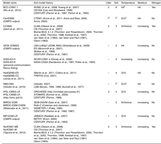
2.1 Earth system models
ESM outputs were drawn from CMIP5 because they used common simulation proto-cols enabling direct comparisons between models. One of the goals of CMIP5 is to facilitate benchmarking of ESMs through the historical simulation protocol, which has a prescribed time series of atmospheric CO2mixing ratios and land use change (Taylor
5
et al., 2011). ESMs were selected from the CMIP5 repository based on the availability of soil carbon predictions and consultation with the modeling centers.
The model structure for terrestrial decomposition across ESMs is relatively uniform (Table 1). The soil carbon sub-models in all ESMs represent decomposition as a first-order decay process involving 1–9 dead (soil or litter) carbon pools. The temperature
10
sensitivity of decomposition in most ESMs is described by theQ10 or Arrhenius
equa-tions, which are functionally similar (Lloyd and Taylor, 1994; Davidson and Janssens, 2006). The Q10 function describes the factor of increase (Q10) in decomposition rate
for a 10◦
C increase in temperature (T) from the initial temperature (T0), such that
Q10(T)=Q
(T−T0)/10
10 . However, in BCC-CSM1.1 and GFDL-ESM2G, decomposition rate
15
increases up to some optimal temperature and then decreases (Parton et al., 1987; Ji et al., 2008; Shevliakova et al., 2009). In addition, the soil respiration response to temperature in GISS-E2 is a linear fit to data from Del Grosso et al. (2005) up to 30◦C, within the noise of the data, with a plateau above 30◦C. In all of the models, decomposi-tion sensitivity to moisture either increases monotonically with increasing soil moisture
20
or increases up to some optimum moisture level and then decreases. Nearly half of the ESMs include nitrogen interactions with soil carbon.
We downloaded soil carbon, litter carbon, annual net primary production (NPP), soil temperature, and total soil water from the historical simulation, where available, for each ESM (cSoil, cLitter, npp, tsl,andmrso, respectively, from the CMIP5 variable list).
25
BGD
9, 14437–14473, 2012
Soil carbon drivers and benchmarks in Earth system models
K. E. O. Todd-Brown et al.
Title Page
Abstract Introduction
Conclusions References
Tables Figures
◭ ◮
◭ ◮
Back Close
Full Screen / Esc
Printer-friendly Version Interactive Discussion
Discussion
P
a
per
|
Dis
cussion
P
a
per
|
Discussion
P
a
per
|
Discussio
n
P
a
per
|
totals since there is no respiration from this pool in the two models which report this variable (CCSM4 and NorESM1). INM-CM4 did not report NPP directly, so we derived NPP from gross primary production and autotrophic respiration (gpp and ra from the variable list). The monthly means for all variables from 1995–2005 were averaged for each grid cell to generate an overall mean for comparison to the HWSD and to use as
5
drivers for our reduced complexity model (see below). Soil temperatures were reported for each soil layer but only the top 10 cm mean was used in this analysis. Land area was calculated from the grid area modified by the land cover for each model (areacella andsftlf from the variable list, respectively) where available. Any grid cells reported to be centered at the poles were dropped from the analysis. All ensembles were averaged
10
for each model; however, the some variables were in all ensembles for a given model at the time of download. For example, GISS-E2-R reportedcSoil but nottsl for ensemble r1i1p1 but did report both variables for ensemble r4i1p3.
We performed a hierarchical cluster analysis and found that ESMs from the same climate center generated very similar distributions of soil carbon (Fig. S1). Clusters
15
were constructed using complete linkage of the Euclidian distances between the global soil carbon distributions for each model. Models from the same climate center always showed more than 90 % relative similarity and included the following pairs: GISS-E2 H and R, HadGEM2 ES and CC, IPSL-CM5 (LR) A and B, MIROC-ESM CHEM and base model, and finally NorESM1 ME and M. Therefore model outputs within each of these
20
pairs were averaged prior to further analysis.
ESMs do not report the depth of carbon in the soil profile to CMIP5, making direct comparison with empirical estimates of soil carbon difficult. For our analysis, we as-sumed that all soil carbon was contained with the top 1 m. We recommend that future model inter-comparison projects request soil carbon output from model simulations
25
BGD
9, 14437–14473, 2012
Soil carbon drivers and benchmarks in Earth system models
K. E. O. Todd-Brown et al.
Title Page
Abstract Introduction
Conclusions References
Tables Figures
◭ ◮
◭ ◮
Back Close
Full Screen / Esc
Printer-friendly Version Interactive Discussion
Discussion
P
a
per
|
Dis
cussion
P
a
per
|
Discussion
P
a
per
|
Discussio
n
P
a
per
|
2.2 Datasets
The HWSD provided empirical estimates of global soil carbon stocks to validate ESM predictions. The HWSD is a product of the Food and Agriculture Organization of the United Nations and the Land Use Change and Agriculture Program of the Interna-tional Institute for Applied Systems Analysis. The HWSD aggregates data from the
5
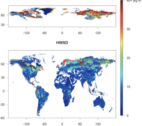
European Soil Database (ESB, 2004), the Soil Map of China (Shi et al., 2004), re-gional soil and terrain databases (Sombroek, 1984), and the Soil Map of the World (FAO/IIASA/ISRIC/ISSCAS/JRC, 2012). Soil carbon stocks were calculated from bulk densities and organic carbon concentrations given in the HWSD for the top 1 m of soil at 0.5◦×0.5◦resolution (Fig. 1). Bulk density estimates were derived from soil texture;
10
however, this approach is not appropriate for high carbon soils (Saxton et al., 1986; FAO/IIASA/ISRIC/ISSCAS/JRC, 2012). Therefore, we replaced Histosol and Andisol bulk densities with values from World Inventory of Soil Emission Potentials (Batjes, 1996).
Because high latitude soils contain a large fraction of global soil carbon, we also
15
validated ESM predictions of soil carbon in high latitudes with the NCSCD, which is an independent survey of soil carbon in this region (Tarnocai et al., 2009). The NCSCD covers 18.8×10⁶km2, including areas with different geological histories and stages of soil development. We used the 1◦×1◦soil carbon data product for the first meter of soil (Fig. 1). The spatial and soil data used to develop this database were collected during
20
the last 60 yr and originated from a variety of sources.
Quantitative uncertainty analyses for the HWSD and NCSCD have not been per-formed and would be a challenge to construct because of the diverse data sources involved. However, some estimate of uncertainty is essential to provide a range within which model projections are expected to fall. To generate such a range for the total soil
25
BGD
9, 14437–14473, 2012
Soil carbon drivers and benchmarks in Earth system models
K. E. O. Todd-Brown et al.
Title Page
Abstract Introduction
Conclusions References
Tables Figures
◭ ◮
◭ ◮
Back Close
Full Screen / Esc
Printer-friendly Version Interactive Discussion
Discussion
P
a
per
|
Dis
cussion
P
a
per
|
Discussion
P
a
per
|
Discussio
n
P
a
per
|
apply to global or regional totals, and uncertainties for individual grid cells are likely to be larger.
For the HWSD, the major sources of error are related to analytical measurement of soil carbon, variation in carbon content within a soil type, and mapping of soil types. Analytical measurements of soil carbon concentrations are generally precise, but
mea-5
surements of soil bulk density are more uncertain and may contribute to CI95 values
that are ±15 % of the mean carbon content for a given soil profile. Soil types in the HWSD are defined based on Food and Agriculture Organization soil taxonomic units that are assumed to experience similar histories of soil forming factors such as cli-mate, vegetation, disturbance, topography, and parent material. Batjes (1997) reported
10
quartiles of soil carbon content for 23 soil taxonomic units based on 18 to 1270 soil profiles per unit. These quartiles suggest that soil carbon content is approximately log-normally distributed, allowing for calculation of CI95 values for each soil unit following
log-transformation. When back transformed, CI95 ranged from 6 to 33 % below the me-dian to 6 to 48 % above the meme-dian, with an average CI95of 14 % below to 17 % above
15
the median across all 23 units.
The final major source of HWSD uncertainty relates to the mapping of soil units and scaling of soil maps to 0.5◦. Soil taxonomic units and associated carbon contents were spatially extrapolated using expert knowledge informed by topography, geology, and vegetation (usually based on aerial photography) Original soil maps were drawn at 1 :
20
1 000 000 or 1 : 5 000 000 spatial resolution and scaled up in the HSWD by classifying each 0.5◦grid cell according to its dominant soil unit. We assumed that the uncertainty associated with mapping and scaling is similar in magnitude to measurement error and spatial variation, with a CI95 of approximately ±15 % of the mean. To estimate
an overall CI95 for the HWSD, we assumed that variation in soil carbon content within
25
soil taxonomic units already includes analytical error, and that median carbon content within a soil unit is extrapolated by multiplying by the area of the unit. Thus the CI95
BGD
9, 14437–14473, 2012
Soil carbon drivers and benchmarks in Earth system models
K. E. O. Todd-Brown et al.
Title Page
Abstract Introduction
Conclusions References
Tables Figures
◭ ◮
◭ ◮
Back Close
Full Screen / Esc
Printer-friendly Version Interactive Discussion
Discussion
P
a
per
|
Dis
cussion
P
a
per
|
Discussion
P
a
per
|
Discussio
n
P
a
per
|
891 to 1657 Pg C. This level of uncertainty is consistent with other empirical estimates of global soil carbon stocks that range from 1220 to 1576 Pg C (Sombroek et al., 1993; Eswaran et al., 1993; Jobbagy and Jackson, 2000).
For the NCSCD, the uncertainties vary by geographic region. The North American portion of the dataset is based on analysis of 1169 pedons producing a medium to high
5
confidence rating (66–80 %). Thus we estimate the CI95for the North American portion
of the NCSCD to be 165±17 Pg C, corresponding to ±10 % of the mean. In Eurasia, soil carbon estimates are based on fewer pedons (591) plus 90 peat cores producing a low to medium confidence rating (33–66 %). Therefore we estimate the CI95 for the
Eurasian region to be 331±99 Pg C, or±30 % of the mean. Carbon in Yedoma deposits
10
and river deltas was estimated independently using surveyed depth information where available. This deeper soil carbon had the lowest confidence rating but contributes only ∼1 % or 5 Pg of the database total; therefore we allow for a CI95 of 5±5 Pg C on this estimate. Together, these uncertainty estimates yield an overall CI95 of 501±121 Pg C for the first meter of soil.
15
To evaluate ESM soil carbon predictions across biomes, we aggregated HWSD esti-mates and model predictions of soil carbon within biomes. The biome map was based on the land cover data product from the MODIS/TERRA-AQUA mission (NASA LP DAAC, 2008) (Fig. S2). We assigned one of 16 land cover types to each 1◦×1◦grid cell by taking the most common land cover from the original underlying 0.05◦
×0.05◦grid.
20
Each 1◦×1◦ grid cell was assigned to one of 9 biomes: tundra, boreal forest, tropical rainforest, temperate forest, desert and scrubland, grasslands and savannas, cropland and urban, snow and ice, or permanent wetland. Details for the biome construction can be found in Fig. S2.
2.3 Regridding approach
25
BGD
9, 14437–14473, 2012
Soil carbon drivers and benchmarks in Earth system models
K. E. O. Todd-Brown et al.
Title Page
Abstract Introduction
Conclusions References
Tables Figures
◭ ◮
◭ ◮
Back Close
Full Screen / Esc
Printer-friendly Version Interactive Discussion
Discussion
P
a
per
|
Dis
cussion
P
a
per
|
Discussion
P
a
per
|
Discussio
n
P
a
per
|
outputs to 1◦
×1◦ down-scales the models while up-scaling the data (Table 2). The uniform grid size allowed for direct comparisons without differences in sample size.
2.4 Reduced complexity models
We developed reduced complexity models to evaluate the drivers of modeled soil car-bon variability and facilitate comparisons between ESMs. These reduced complexity
5
models consisted of a single pool of soil carbon driven by NPP, soil temperature, and soil moisture (Figs. S3–S5). The rationale for this approach is that we can quantify the relationship between driving variables and soil carbon outputs for each model and then compare these relationships across models. Driving variables for the reduced models are taken from ESM annual means of NPP, soil temperature (T, top 10-cm mean), and
10
total soil water content (W) over the period 1995–2005.
Our reduced models assume that the soil carbon pool is at steady state, such that NPP inputs equal outputs from heterotrophic respiration (R):
0=dC
dt =NPP−R
15
For the simplest reduced model, we assumed that soil respiration is directly propor-tional to the soil carbon pool with rate constantk (Olson, 1963; Parton et al., 1987)
R=kC
Combining the two above equations yields the simplest reduced model, Eq. (1), in
20
which soil carbon is proportional to NPP and inversely proportional to decomposition rate (k):
C=NPP
k (1)
We formulated a second reduced model, Eq. (2), in which soil respiration depends
25
on soil temperature (T) according to a Q10 function with an initial temperature of 15
BGD
9, 14437–14473, 2012
Soil carbon drivers and benchmarks in Earth system models
K. E. O. Todd-Brown et al.
Title Page
Abstract Introduction
Conclusions References
Tables Figures
◭ ◮
◭ ◮
Back Close
Full Screen / Esc
Printer-friendly Version Interactive Discussion
Discussion
P
a
per
|
Dis
cussion
P
a
per
|
Discussion
P
a
per
|
Discussio
n
P
a
per
|
(Lloyd and Taylor, 1994):
C= NPP
kQ(10T−15)/10
(2)
A third reduced model, Eq. (3), includes a moisture modifier which monotonically in-creases with total soil water content (W) according to an exponential function, wherea
5
is a normalization parameter andbis the scaling exponent:
C= NPP
kQ(10T−15)/10aWb
(3)
The parametersk,Q10,a, and b in each reduced model were optimized on the ESM soil carbon predictions and driving variables by grid cell. For the optimization, we
10
used a constrained Broyden-Fletcher-Goldfarb-Shanno algorithm (Byrd et al., 1995), a quasi-Newtonian method, as implemented in R 2.13.1 (R Development Core Team, 2011). Broyden-Fletcher-Goldfarb-Shanno was selected for parameter fitting because of its robust convergence and short run time. We ran the optimization with the fol-lowing constraints: ak∈(10−4, 104), Q10∈(10−4, 5), b∈(−3, 3). The initial parameter
15
estimates wereak=0.1,Q10=1,b=0. We used root mean squared error (RMSE) as
the measure function.
2.5 Statistical analyses
ESM predictions were compared to datasets using Pearson’s correlation, root mean squared error (RMSE), and Taylor scores using R 2.13.1 (R Development Core Team,
20
2011). The Taylor score (TS) combines the Pearson’s correlation (c) and standard
de-viation (σ) of the model results (m) compared to the data (d):
TS(d,m)= 4 [1+c(d,m)]
σ(m)/σ(d)+σ(d)/σ(m)2
1+cmax
BGD
9, 14437–14473, 2012
Soil carbon drivers and benchmarks in Earth system models
K. E. O. Todd-Brown et al.
Title Page
Abstract Introduction
Conclusions References
Tables Figures
◭ ◮
◭ ◮
Back Close
Full Screen / Esc
Printer-friendly Version Interactive Discussion
Discussion
P
a
per
|
Dis
cussion
P
a
per
|
Discussion
P
a
per
|
Discussio
n
P
a
per
|
wherecmaxis the maximum correlation attainable, assumed to be 1 in this case (Taylor,
2001). Biome aggregated totals were compared to the HWSD using linear regression.
3 Results
3.1 Global soil carbon
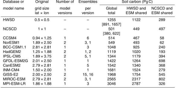
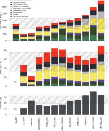
The mean (± SD) global soil carbon reported across all ESMs was 1480±740 Pg,
5
whereas the global soil carbon in the HWSD was 1255 Pg with a CI95 from 891–
1657 Pg (Table 2, Fig. 2). CCSM4 reported the lowest total at 514 Pg C and MPI-ESM-LR the highest at 3046 Pg C. Examining only the area shared by each ESM and the HWSD reduces the global carbon totals but does not substantially change the rank order of the models (Table 2). CCSM4 and NorESM1 underestimated global soil
10
carbon stocks by up to 50 %, whereas GISS-E2, MIROC-ESM, and MPI-ESM-LR over-estimated global soil carbon stocks anywhere from 55 % to 140 %. The other models predicted global soil carbon totals that were within 25 % of the HWSD mean and fell within its preliminary CI95.
High latitude soil carbon was generally underestimated by the ESMs, and the model
15
rankings change when examining only high-latitude soil carbon as defined by grid cells in the NCSCD (Table 2, Fig. S6). CCSM4 and NorESM1 predicted just over 10 % of the expected total soil carbon in the high latitudes. HadGEM2, BCC-CSM1.1, INM-CM4, MPI-ESM, CanESM2 also predicted soil carbon totals below the preliminary CI95 for
the NCSCD. In contrast, GFDL-ESM2G and MIROC-ESM overestimated high latitude
20
soil carbon stocks by 45–60 %. Only IPSL-CM5 and GISS-E2 predictions fell within the CI95for the NCSCD.
3.2 Spatial distribution of soil carbon
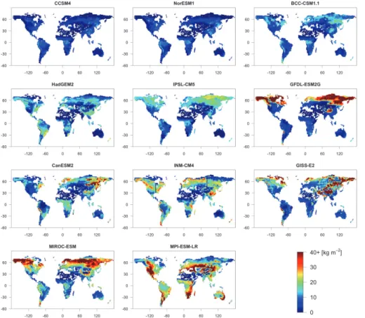
The predicted spatial distribution of soil carbon stocks varied widely among the ESMs (Fig. 3). CCSM4 and NorESM1 had the lowest overall soil carbon densities, but showed
BGD
9, 14437–14473, 2012
Soil carbon drivers and benchmarks in Earth system models
K. E. O. Todd-Brown et al.
Title Page
Abstract Introduction
Conclusions References
Tables Figures
◭ ◮
◭ ◮
Back Close
Full Screen / Esc
Printer-friendly Version Interactive Discussion
Discussion
P
a
per
|
Dis
cussion
P
a
per
|
Discussion
P
a
per
|
Discussio
n
P
a
per
|
high densities in Northern South America, Central Africa, Eastern Asia, and Eastern North America. HadGEM2, BCC-CSM1.1, and INM-CM4 showed a broader range of soil carbon densities with high densities in North America, Western South America, Central Africa, Southeastern Asia, and Northern Eurasia excluding Siberia. HadGEM2 also showed elevated soil carbon in Southeastern South America. CanESM2 predicted
5
high soil carbon in Northeastern North America, Northern Europe, Northeastern Asia, Central Africa, and Eastern South America. GFDL-ESM2G and MIROC-ESM showed uniformly high carbon densities across all high northern latitudes and around the Ti-betan plateau. GISS-E2 predicted a region of high soil carbon across the northern latitudes of North America and northern Europe, as well as another area of high soil
10
carbon from northeastern to southwestern Asia. MPI-ESM-LR showed an inverse pat-tern compared with the other ESMs; soil carbon peaked in the mid-latitudes across Asia, Western North America, Eastern Africa, Southern South America, and Southern Coastal Australia.
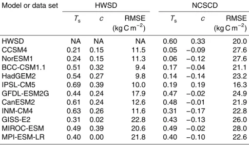
There was generally poor agreement between the ESMs and the HWSD soil carbon
15
distribution (Table 3). Across all common grid cells, ESMs had Pearson correlations between 0.00 and 0.39 with a highly variable RMSE between 9.4 and 22.8 kg C m−2
and Taylor scores ranging from 0.21 to 0.69. Model agreement with the high latitude NCSCD dataset was even worse (correlations between−0.17 and 0.19, Taylor scores between 0.05 and 0.49, and RMSE between 16.3 and 28.0 kg C m−2
). Agreement
20
between the HWSD and NCSCD datasets was also low (correlation of 0.33, RMSE of 20.0 kg C m−2, and Taylor score of 0.60), although better than any ESM agreement with the NCSCD dataset.
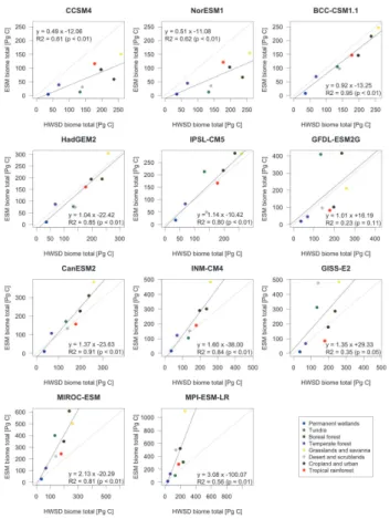
ESM agreement with the HWSD generally improved at the biome level (Fig. 4). BCC-CSM1.1 and CanESM2 stood out as being highly correlated with HWSD (R2>0.90,
25
BGD
9, 14437–14473, 2012
Soil carbon drivers and benchmarks in Earth system models
K. E. O. Todd-Brown et al.
Title Page
Abstract Introduction
Conclusions References
Tables Figures
◭ ◮
◭ ◮
Back Close
Full Screen / Esc
Printer-friendly Version Interactive Discussion
Discussion
P
a
per
|
Dis
cussion
P
a
per
|
Discussion
P
a
per
|
Discussio
n
P
a
per
|
HadGEM2 over-estimated soil carbon in grasslands and savanna. ISPL-CM5 gen-erally over-estimated all biomes except deserts and scrublands, which were under-estimated. INM-CM4 over-estimated grasslands, savanna, boreal forests, croplands, and urban. MIROC-ESM consistently over-estimated all biomes. Both CCSM4 and NorESM1 were moderately correlated with the HWSD (0.55> R2>0.50, p <0.01)
5
consistently under-estimating biome totals with notable under-estimations in the tun-dra, boreal forest, desert, and scrubland biomes. Biome totals from MPI-ESM-LR were also moderately correlated with the HWSD (R2=0.56,p=0.01), but this model consis-tently over-estimated biome totals, particularly grasslands and savanna. GFDL-ESM2G and GISS-E2 did not correlate significantly (p >0.05) with the HWSD on the biome
10
level. GFDL-ESM2G over-estimated biome totals from tundra and boreal forests and under-estimated those of tropical rainforests, croplands, and urban. GISS-E2 over-estimated biome totals in desert, scrubland, grasslands, savanna, tundra, and boreal forests and under-estimated tropical rainforests.
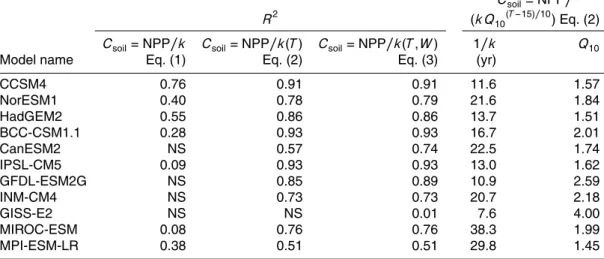
3.3 Drivers of ESM variability
15
The spatial variability in all but two ESMs was well explained by the reduced complexity model (Eq. 2) driven by NPP and soil temperature (R2>0.73). Turnover times (1/k) for global soil carbon across the ESMs ranged from 11 to 39 yr, andQ10values ranged
from 1.5 to 2.6 (T0=15
◦
C) (Table 4). The reduced complexity model for CanESM2 was the only one improved by the addition of soil moisture (Eq. 3) withR2 increasing
20
from 0.57 to 0.74. Soil carbon outputs from GISS-E2 (R2<0.05) and MPI-ESM-LR (R2<0.51) were not well explained by any of the reduced complexity models.
4 Discussion
Because belowground carbon stocks are so large, accurate models of the soil car-bon cycle are essential for predicting carcar-bon-climate feedbacks in the future. As far
BGD
9, 14437–14473, 2012
Soil carbon drivers and benchmarks in Earth system models
K. E. O. Todd-Brown et al.
Title Page
Abstract Introduction
Conclusions References
Tables Figures
◭ ◮
◭ ◮
Back Close
Full Screen / Esc
Printer-friendly Version Interactive Discussion
Discussion
P
a
per
|
Dis
cussion
P
a
per
|
Discussion
P
a
per
|
Discussio
n
P
a
per
|
as we know, our analysis is the first to benchmark soil carbon outputs from ESMs against empirical data at the global scale and explore the possible factors contributing to differences among models. Although some models predicted reasonable global soil carbon totals, only a few were able to match biome totals and none were able to repro-duce grid-scale distributions of soil carbon. Better performance at the biome to global
5
scale may be due to aggregation of variable environmental conditions within biomes that were influential in the grid scale comparison. At the grid scale in particular, there are a number of factors that may have contributed to the poor agreement between model predictions and empirical data. These factors include (1) uncertainties in the data, (2) incorrect representation of soil carbon drivers in the models (e.g. NPP,
tem-10
perature, moisture), (3) incorrect model parameterization of the soil carbon response to drivers, and (4) incorrect model structure. Addressing these issues will be essential for increasing confidence in ESM predictions of soil carbon in the future.
Our ability to evaluate model performance relies on high quality empirical data with associated estimates of uncertainty. Despite their comprehensiveness, a lack of
quanti-15
tative uncertainty estimates for the HWSD and NCSCD datasets constrains our bench-marking analyses. Although the models clearly disagree among themselves, knowing which model predictions diverge from the data is difficult to assess without a formal analysis of uncertainty in the data. Our preliminary analyses based on expert opin-ion indicate that uncertainty in empirical estimates of soil carbon stocks could exceed
20
770 Pg C at the global scale, an amount similar to the entire atmospheric pool of car-bon. In addition to these preliminary uncertainty estimates, we found that the spatial correlation between the HWSD and the NCSCD was only 0.33 where they overlap. This value was higher than any model-data correlation for the same region, but it clearly in-dicates that there is room for improvement in the empirical estimates.
25
BGD
9, 14437–14473, 2012
Soil carbon drivers and benchmarks in Earth system models
K. E. O. Todd-Brown et al.
Title Page
Abstract Introduction
Conclusions References
Tables Figures
◭ ◮
◭ ◮
Back Close
Full Screen / Esc
Printer-friendly Version Interactive Discussion
Discussion
P
a
per
|
Dis
cussion
P
a
per
|
Discussion
P
a
per
|
Discussio
n
P
a
per
|
the driving variables for soil carbon in the models. For example, soil carbon stocks are positively related to NPP (Table 4), which varies by a factor of 3.4 across the models. The spatial distribution of NPP was similarly highly variable across models (Fig. S3). In contrast, mean annual soil temperature was relatively consistent between the EMSs (Fig. S4). Empirical models, using field measurements of NPP extrapolated globally
5
based on environmental parameters indicate that global NPP is approximately 54.0± 10.5 Pg C yr−1(mean±standard deviation), roughly in agreement with remote sensing estimates (Ito, 2011). CCSM, BCC-CSM1.1, HadGEM2, CanESM2, INM-CM4, GISS-E2, and MIROC-ESM all predicted global NPP within two standard deviations of the Ito (2011) estimate, ranging from 46.3 to 72.9 Pg C yr−1. The remaining 5 models fell
10
outside this range, which may affect their predictions of soil carbon. Thus, improving model predictions of driving variables like NPP, and to a lesser extent temperature and soil moisture, could also improve soil carbon predictions.
Another potential source of disagreement between models is the response to driving variables such as NPP, temperature, and soil moisture. This response is determined by
15
model parameterization, which we summarized by calculating global turnover times for soil carbon (Fig. 2, Table 4). Based on estimates of heterotrophic soil respiration and soil carbon stocks, global turnover times for soil carbon range from 18.5 yr (Amundson, 2001) to 32 yr (Raich and Schlesinger, 1992). NorESM1, CanESM2, and INM-CM4 turnover times fall within this range, whereas the other models do not. Correctly
pa-20
rameterizing soil carbon models remains a challenge because important mechanisms can operate at spatial scales much smaller than an ESM grid cell. Differences in soil texture and topography at small scales may lead to non-linear effects on soil carbon storage that are not well described by the average characteristics of a grid cell. For instance, relatively small scale topographic variations are associated with peatland
for-25
mation (Gorham, 1991; Koven et al., 2011).
BGD
9, 14437–14473, 2012
Soil carbon drivers and benchmarks in Earth system models
K. E. O. Todd-Brown et al.
Title Page
Abstract Introduction
Conclusions References
Tables Figures
◭ ◮
◭ ◮
Back Close
Full Screen / Esc
Printer-friendly Version Interactive Discussion
Discussion
P
a
per
|
Dis
cussion
P
a
per
|
Discussion
P
a
per
|
Discussio
n
P
a
per
|
to validate the accuracy of Earth system models. In order to have confidence in future predictions, the models must correctly represent the mechanisms and drivers of soil carbon change. Models with incorrect mechanisms or drivers could be tuned to make correct predictions of current soil carbon stocks, but might generate different predic-tions of soil carbon stocks over time.
5
We initially hypothesized that models with more pools would have greater flexibility and capture more of the spatial variation in soil carbon. However, the structural features that we examined did not clearly relate to differences in ESM agreement with empirical data (Tables 1 and 3). We saw no pattern in ESM-data agreement with respect to number of soil carbon pools or temperature and moisture sensitivity functions, nor with
10
respect to presence of a nitrogen component. Furthermore, our reduced complexity model (Eq. 3) explained most of the variation in 9 of 11 model types (0.73< R2<
0.93). This result confirms that, despite different soil carbon predictions, most of the models share a similar underlying structure. Such similarity means that the models likely make similar assumptions about the mechanisms regulating soil carbon cycling.
15
If these underlying assumptions are incorrect or incomplete, the resulting errors will be present in all of the models.
CanESM2, MPI-ESM-LR, and GISS-E2 are three exceptions that were not well ex-plained by our reduced complexity model (Eq. 2) driven by NPP and soil temperature (Table 4), and thus may be examples of models with structural differences. CanESM2
20
was the only model in which soil water content contributed to the explanatory power of the reduced complexity model (R2 improved from 0.57 to 0.74). This dependency on soil water content could be explained by the biome-specific turnover time in CanESM2. Since biomes are partially determined by precipitation, the effect of biome-specific turnover times may have been reflected in an increased sensitivity to soil moisture
25
BGD
9, 14437–14473, 2012
Soil carbon drivers and benchmarks in Earth system models
K. E. O. Todd-Brown et al.
Title Page
Abstract Introduction
Conclusions References
Tables Figures
◭ ◮
◭ ◮
Back Close
Full Screen / Esc
Printer-friendly Version Interactive Discussion
Discussion
P
a
per
|
Dis
cussion
P
a
per
|
Discussion
P
a
per
|
Discussio
n
P
a
per
|
predictions from other models. GISS-E2 outputs were poorly explained by the reduced complexity model (R2<0.01). Unlike other models, GISS-E2 showed a unique discon-nect between NPP and soil carbon which could be due to differences in the way plant biomass is allocated to liter in the models. However, as with MPI-ESM-LR we cannot offer a definitive explanation for the poor fit.
5
Although we did not identify major structural differences among models, they may all be missing key processes governing long term carbon storage that may affect model-data agreement. These key governing components may include aggregate interactions (Six et al., 2000), microbial dynamics (Todd-Brown et al., 2010), cryoturbation (Koven et al., 2011), syngenetic soil formation (Shur et al., 2004), and rare substrate formation
10
(Allison, 2006). For example, microbial uptake of carbon substrates is non-linearly de-pendent on substrate concentration, whereas current models use a linear dependence (Schimel and Weintraub, 2003; German et al., 2011). Representing these processes in the structure of soil carbon models remains a major challenge. A multi-scale ap-proach is required to determine which processes are important at the global scale. For
15
example, slope affects soil drainage and thus moisture. Some grid cells may have an average slope near zero, but include topographic variation and low-lying areas with water-logged soils and high rates of soil carbon accumulation at the kilometer scale.
5 Conclusions
Overall, we found that that soil carbon sub-models in ESMs have difficulty representing
20
present-day stocks of soil carbon, particularly at the scale of a model grid cell. Despite similar overall structures, the models do not agree among themselves or with empirical data on the global distribution of soil carbon. Reconciling this disagreement will require a range of approaches, including better prediction of soil carbon drivers, more accurate model parameterization, and more comprehensive representation of critical biological
25
BGD
9, 14437–14473, 2012
Soil carbon drivers and benchmarks in Earth system models
K. E. O. Todd-Brown et al.
Title Page
Abstract Introduction
Conclusions References
Tables Figures
◭ ◮
◭ ◮
Back Close
Full Screen / Esc
Printer-friendly Version Interactive Discussion
Discussion
P
a
per
|
Dis
cussion
P
a
per
|
Discussion
P
a
per
|
Discussio
n
P
a
per
|
of soil carbon stocks that are used to benchmark ESMs. If this uncertainty is too high for rigorous model comparison, additional measurements of soil carbon stocks may be required in some regions of the world. Addressing these issues will improve our ability to predict the response of the carbon cycle to climate change and inform policymakers about the potential impacts of carbon emissions.
5
Supplementary material related to this article is available online at: http://www.biogeosciences-discuss.net/9/14437/2012/
bgd-9-14437-2012-supplement.pdf.
Acknowledgements. We thank Shishi Lui and Yaxing Wei for their work with the HWSD, as well as Yufang Jin for her work with the NCSCD data set. This research was funded by grants from
10
the NSF Advancing Theory in Biology program, the Decadal and Regional Climate Prediction using Earth System Models (EaSM; AGU-1048890) program, and the Office of Science (BER), US Department of Energy.
We acknowledge the World Climate Research Programme’s Working Group on Coupled Mod-eling, which is responsible for CMIP, and we thank the climate modeling groups (listed in Table
15
S1) for producing and making available their model output. For CMIP, the US Department of Energy’s Program for Climate Model Diagnosis and Intercomparison provided coordinating sup-port and led development of software infrastructure in partnership with the Global Organization for Earth System Science Portals.
The authors have no potential conflicts of interest to declare.
20
References
Allison, S. D.: Brown Ground: a soil carbon analogue for the green world hypothesis?, Am. Nat., 167, 619–627, 2006.
Amundson, R.: The carbon budget in soils, Annu. Rev. Earth Planet. Sc., 29, 535–562, 2001. Arora, V.: Simulating energy and carbon fluxes over winter wheat using coupled land surface
25
BGD
9, 14437–14473, 2012
Soil carbon drivers and benchmarks in Earth system models
K. E. O. Todd-Brown et al.
Title Page
Abstract Introduction
Conclusions References
Tables Figures
◭ ◮
◭ ◮
Back Close
Full Screen / Esc
Printer-friendly Version Interactive Discussion
Discussion
P
a
per
|
Dis
cussion
P
a
per
|
Discussion
P
a
per
|
Discussio
n
P
a
per
|
Arora, V. K. and Boer, G. J.: A parameterization of leaf phenology for the terrestrial ecosystem component of climate models, Glob. Change Biol., 11, 39–59, 2005.
Arora, V. K., Scinocca, J. F., Boer, G. J., Christian, J. R., Denman, K. L., Flato, G. M., Kharin, V. V., Lee, W. G., and Merryfield, W. J.: Carbon emission limits required to satisfy future representative concentration pathways of greenhouse gases, Geophys. Res. Lett., 38,
5
L05805, doi:10.1029/2010GL046270, 2011.
Batjes, N.: Total carbon and nitrogen in the soils of the world, Eur. J. Soil Sci., 47, 151–163, 1996.
Batjes, N. H.: A world dataset of derived soil properties by FAO–UNESCO soil unit for global modelling, Soil Use Manage., 13, 9–16, 1997.
10
Bolker, B. M., Pacala, S. W., and Parton, W. J.: Linear analysis of soil decomposition: insights from the century model, Ecol. Appl., 8, 425–439, 1998.
Bonan, G. B.: Land-atmosphere CO2 exchange simulated by a land surface process model coupled to an atmospheric general circulation model, J. Geophys. Res., 100, 2817–2831, 1995.
15
Bonan, G. B.: A land surface model (LSM version 1.0) for ecological, hydrological and atmospheric studies: technical discription and user’s guide, NCAR technical note NCAR/TN-417+STR, Climate and global dynamics division, National Center for At-mospheric Research, Boulder, CO, available at: http://nldr.library.ucar.edu/collections/ technotes/asset-000-000-000-229.pdf (last access: August 2012), 1996.
20
Bunnell, F. L., Tait, D. E. N., Flanagan, P. W., and Van Clever, K.: Microbial respiration and substrate weight loss – I: a general model of the influences of abiotic variables, Soil Biol. Biochem., 9, 33–40, 1977.
Byrd, R. H., Lu, P., Nocedal, J., and Zhu, C.: A limited memory algorithm for bound constrained optimization, SIAM J. Sci. Comput., 16, 1190–1208, 1995.
25
Cao, M. and Woodward, F. I.: Net primary and ecosystem production and carbon stocks of terrestrial ecosystems and their responses to climate change, Glob. Change Biol., 4, 185– 198, 1998.
Coleman, K. and Jenkinson, D. S.: ROTHC-26.3, A model for the turnover of carbon in soils, Tech. Rep., available at: http://www.rothamsted.ac.uk/aen/carbon/mod26 3 dos.pdf (last
ac-30
cess: October 2012), 1999.
BGD
9, 14437–14473, 2012
Soil carbon drivers and benchmarks in Earth system models
K. E. O. Todd-Brown et al.
Title Page
Abstract Introduction
Conclusions References
Tables Figures
◭ ◮
◭ ◮
Back Close
Full Screen / Esc
Printer-friendly Version Interactive Discussion
Discussion
P
a
per
|
Dis
cussion
P
a
per
|
Discussion
P
a
per
|
Discussio
n
P
a
per
|
Sitch, S., Totterdell, I., Wiltshire, A., and Woodward, S.: Development and evaluation of an Earth-System model – HadGEM2, Geosci. Model Dev., 4, 1051–1075, doi:10.5194/gmd-4-1051-2011, 2011.
Cox, P. M.: Description of the “TRIFFID” Dynamic Global Vegetation Model, Technical Note 24, Hadley Center, available at: http://climate.uvic.ca/model/common/HCTN 24.pdf (last access:
5
August 2012), 2001.
Cramer, W., Bondeau, A., Woodward, F. I., Prentice, I. C., Betts, R. A., Brovkin, V., Cox, P. M., Fisher, V., Foley, J. A., Friend, A. D., Kucharik, C., Lomas, M. R., Ramankutty, N., Sitch, S., Smith, B., White, A., and Young-Molling, C.: Global response of terrestrial ecosystem struc-ture and function to CO2 and climate change: results from six dynamic global vegetation
10
models, Glob. Change Biol., 7, 357–373, 2001.
Davidson, E. A. and Janssens, I. A.: Temperature sensitivity of soil carbon decomposition and feedbacks to climate change, Nature, 440, 165–173, 2006.
Del Grosso, S., Parton, W., Mosier, A., Holland, E., Pendall, E., Schimel, D., and Ojima, D.: Modeling soil CO2emissions from ecosystems, Biogeochemistry, 73, 71–91, 2005.
15
Doney, S. C., Lindsay, K., Fung, I., and John, J.: Natural variability in a stable, 1000-yr global coupled climate–carbon cycle simulation, J. Climate, 19, 3033–3054, 2006.
ESB: European Soil Database (vs 2.0), European Commission – JRC – Institute for Environ-ment and Sustainability, European Soil Bureau, Ispra, Italy, 2004.
Eswaran, H., Van Den Berg, E., and Reich, P.: Organic carbon in soils of the world, Soil Sci.
20
Soc. Am. J., 57, 192–194, 1993.
FAO/IIASA/ISRIC/ISSCAS/JRC: Haromonized World Soil Database (version 1.2), FAO, Rome, Italy and IIASA, Laxenburg, Austria, 2012.
Foley, J. A.: An equilibrium model of the terrestrial carbon budget, Tellus B, 47, 310–319, 1995. Friedlingstein, P., Cox, P., Betts, R., Bopp, L., von Bloh, W., Brovkin, V., Cadule, P., Doney, S.,
25
Eby, M., Fung, I., Bala, G., John, J., Jones, C., Joos, F., Kato, T., Kawamiya, M., Knorr, W., Lindsay, K., Matthews, H. D., Raddatz, T., Rayner, P., Reick, C., Roeckner, E., Schnit-zler, K. G., Schnur, R., Strassmann, K., Weaver, A. J., Yoshikawa, C., and Zeng, N.: Climate– carbon cycle feedback analysis: results from the C4MIP Model intercomparison, J. Climate, 19, 3337–3353, 2006.
30
BGD
9, 14437–14473, 2012
Soil carbon drivers and benchmarks in Earth system models
K. E. O. Todd-Brown et al.
Title Page
Abstract Introduction
Conclusions References
Tables Figures
◭ ◮
◭ ◮
Back Close
Full Screen / Esc
Printer-friendly Version Interactive Discussion
Discussion
P
a
per
|
Dis
cussion
P
a
per
|
Discussion
P
a
per
|
Discussio
n
P
a
per
|
Zhang, M.: The Community Climate System Model Version 4, J. Climate, 24, 4973–4991, 2011.
German, D. P., Chacon, S., and Allison, S.: Substrate concentration and enzyme allocation can affect rates of microbial decomposition, Ecology, 92, 1471–1480, 2011.
Gorham, E.: Northern Peatlands: role in the carbon cycle and probable responses to climatic
5
warming, Ecol. Appl., 1, 182–195, 1991.
Goulden, M. L., Mcmillan, A. M. S., Winston, G. C., Rocha, A. V., Manies, K. L., Harden, J. W., and Bond-Lamberty, B. P.: Patterns of NPP, GPP, respiration, and NEP during boreal forest succession, Glob. Change Biol., 17, 855–871, 2011.
Harden, J. W., Trumbore, S. E., Stocks, B. J., Hirsch, A., Gower, S. T., O’neill, K. P., and
Ka-10
sischke, E. S.: The role of fire in the boreal carbon budget, Glob. Change Biol., 6, 174–184, 2000.
Huang, M., Ji, J., Li, K., Liu, Y., Yang, F., and Tao, B.: The ecosystem carbon accumulation after conversion of grasslands to pine plantations in subtropical red soil of South China, Tellus B, 59, 439–448, 2007.
15
Huntingford, C., Fisher, R. A., Mercado, L., Booth, B. B., Sitch, S., Harris, P. P., Cox, P. M., Jones, C. D., Betts, R. A., Malhi, Y., Harris, G. R., Collins, M., and Moorcroft, P.: Towards quantifying uncertainty in predictions of Amazon “dieback”, Philos. T. Roy. Soc. B, 363, 1857– 1864, 2008.
Ito, A.: A historical meta-analysis of global terrestrial net primary productivity: are estimates
20
converging?, Glob. Change Biol., 17, 3161–3175, 2011.
Ji, J., Huang, M., and Li, K.: Prediction of carbon exchanges between China terrestrial ecosys-tem and atmosphere in 21st century, Sci. China Ser. D: Earth Sci., 51, 885–898, 2008. Jobbagy, E. G. and Jackson, R. B.: The vertical distribution of soil organic carbon and its relation
to climate and vegetation, Ecol. Appl., 10, 423–436, 2000.
25
Jones, C. D., Hughes, J. K., Bellouin, N., Hardiman, S. C., Jones, G. S., Knight, J., Liddi-coat, S., O’Connor, F. M., Andres, R. J., Bell, C., Boo, K. O., Bozzo, A., Butchart, N., Cadule, P., Corbin, K. D., Doutriaux-Boucher, M., Friedlingstein, P., Gornall, J., Gray, L., Halloran, P. R., Hurtt, G., Ingram, W. J., Lamarque, J.-F., Law, R. M., Meinshausen, M., Osprey, S., Palin, E. J., Parsons Chini, L., Raddatz, T., Sanderson, M. G., Sellar, A. A.,
30
BGD
9, 14437–14473, 2012
Soil carbon drivers and benchmarks in Earth system models
K. E. O. Todd-Brown et al.
Title Page
Abstract Introduction
Conclusions References
Tables Figures
◭ ◮
◭ ◮
Back Close
Full Screen / Esc
Printer-friendly Version Interactive Discussion
Discussion
P
a
per
|
Dis
cussion
P
a
per
|
Discussion
P
a
per
|
Discussio
n
P
a
per
|
Kimball, J. S., Thornton, P. E., White, M. A., and Running, S. W.: Simulating forest productivity and surface-atmosphere carbon exchange in the BOREAS study region, Tree Physiol., 17, 589–599, 1997.
Knorr, W.: Annual and interannual CO2exchanges of the terrestrial biosphere: process-based simulations and uncertainties, Global Ecol. Biogeogr., 9, 225–252, 2000.
5
Koven, C. D., Ringeval, B., Friedlingstein, P., Ciais, P., Cadule, P., Khvorostyanov, D., Krinner, G., and Tarnocai, C.: Permafrost carbon-climate feedbacks accelerate global warming, P. Natl. Acad. Sci., 108, 14769–14774, 2011.
Krinner, G., Viovy, N., de Noblet-Ducoudr `e, N., Og `ee, J., Polcher, J., Friedlingstein, P., Ciais, P., Sitch, S., and Prentice, I. C.: A dynamic global vegetation model for
stud-10
ies of the coupled atmosphere-biosphere system, Global Biogeochem. Cy., 19, GB1015, doi:10.1029/2003GB002199, 2005.
Lloyd, J. and Taylor, J. A.: On the temperature dependence of soil respiration, Funct. Ecol., 8, 315–323, 1994.
Lund, M., Lafleur, P. M., Roulet, N. T., Lindroth, A., Christensen, T. R., Aurela, M.,
Cho-15
jnicki, B. H., Flanagan, L. B., Humphreys, E. R., Laurila, T., Oechel, W. C., Olejnik, J., Rinne, J., Schubert, P., and Nilsson, M. B.: Variability in exchange of CO2across 12 northern peatland and tundra sites, Glob. Change Biol., 16, 2436–2448, 2010.
Luo, Y. Q., Randerson, J. T., Abramowitz, G., Bacour, C., Blyth, E., Carvalhais, N., Ciais, P., Dal-monech, D., Fisher, J. B., Fisher, R., Friedlingstein, P., Hibbard, K., Hoffman, F., Huntzinger,
20
D., Jones, C. D., Koven, C., Lawrence, D., Li, D. J., Mahecha, M., Niu, S. L., Norby, R., Piao, S. L., Qi, X., Peylin, P., Prentice, I. C., Riley, W., Reichstein, M., Schwalm, C., Wang, Y. P., Xia, J. Y., Zaehle, S., and Zhou, X. H.: A framework for benchmarking land models, Biogeo-sciences, 9, 3857–3874, doi:10.5194/bg-9-3857-2012, 2012.
The HadGEM2 Development Team: Martin, G. M., Bellouin, N., Collins, W. J.,
Culver-25
well, I. D., Halloran, P. R., Hardiman, S. C., Hinton, T. J., Jones, C. D., McDonald, R. E., McLaren, A. J., O’Connor, F. M., Roberts, M. J., Rodriguez, J. M., Woodward, S., Best, M. J., Brooks, M. E., Brown, A. R., Butchart, N., Dearden, C., Derbyshire, S. H., Dharssi, I., Doutriaux-Boucher, M., Edwards, J. M., Falloon, P. D., Gedney, N., Gray, L. J., Hewitt, H. T., Hobson, M., Huddleston, M. R., Hughes, J., Ineson, S., Ingram, W. J., James, P. M.,
30
BGD
9, 14437–14473, 2012
Soil carbon drivers and benchmarks in Earth system models
K. E. O. Todd-Brown et al.
Title Page
Abstract Introduction
Conclusions References
Tables Figures
◭ ◮
◭ ◮
Back Close
Full Screen / Esc
Printer-friendly Version Interactive Discussion
Discussion
P
a
per
|
Dis
cussion
P
a
per
|
Discussion
P
a
per
|
Discussio
n
P
a
per
|
family of Met Office Unified Model climate configurations, Geosci. Model Dev., 4, 723–757, doi:10.5194/gmd-4-723-2011, 2011.
Moorcroft, P. R., Hurtt, G. C., and Pacala, S. W.: A method for scaling vegetation dynamics: the ecosystem demography model (ED), Ecol. Monogr., 71, 557–586, 2001.
NASA Land Processes Distributed Active Archive Center (LP DAAC): MODIS/Terra+Aqua Land
5
Cover Type Yearly L3 Global 0.05Deg CMG, 2008.
Neff, J. C. and Hooper, D. U.: Vegetation and climate controls on potential CO2, DOC and DON production in northern latitude soils, Glob. Change Biol., 8, 872–884, 2002.
Oleson, K. W., Niu, G. Y., Yang, Z. L., Lawrence, D. M., Thornton, P. E., Lawrence, P. J., Stockli, R., Dickinson, R. E., Bonan, G. B., Levis, S., Dai, A., and Qian, T.: Improvements
10
to the community land model and their impact on the hydrological cycle, J. Geophys. Res., 113, G01021, doi:10.1029/2007JG000563, 2008.
Olson, J. S.: Energy storage and the balance of producers and decomposers in ecological systems, Ecology, 44, 322–331, 1963.
Orchard, V. A. and Cook, F.: Relationship between soil respiration and soil moisture, Soil Biol.
15
Biochem., 15, 447–453, 1983.
Parton, W., Schimel, D., Cole, C., and Ojima, D.: Analysis of factors controlling soil organic-matter levels in Great-Plains Grasslands, Soil Sci. Soc. Am. J., 51, 1173–1179, 1987. Parton, W., Stewart, J., and Cole, C.: Dynamics of C, N, P and S in grassland soils: a model,
Biogeochemistry, 5, 109–131, 1988.
20
Parton, W. J., Running, S. W., and Walker, B.: A toy terrestrial carbon flow model, Tech. Rep. SEE N94-30616 08-45, OIES/UCAR, 1992.
Parton, W., Scurlock, J., Ojima, D., Gilmanov, T., Scholes, R., Schimel, D., Kirchner, T., Me-naut, J., Seastedt, T., Moya, E., Kamnalrut, A., and Kinyamario, J.: Observations and model-ing of biomass and soil organic-matter dynamics for the Grassland Biome Worldwide, Global
25
Biogeochem. Cy., 7, 785–809, 1993.
Phillips, O. L., Aragao, L. E. O. C., Lewis, S. L., Fisher, J. B., Lloyd, J., Lopez-Gonzalez, G., Malhi, Y., Monteagudo, A., Peacock, J., Quesada, C. A., van der Heijden, G., Almeida, S., Amaral, I., Arroyo, L., Aymard, G., Baker, T. R., Banki, O., Blanc, L., Bonal, D., Brando, P., Chave, J., de Oliveira, A. C. A., Cardozo, N. D., Czimczik, C. I., Feldpausch, T. R.,
Fre-30
BGD
9, 14437–14473, 2012
Soil carbon drivers and benchmarks in Earth system models
K. E. O. Todd-Brown et al.
Title Page
Abstract Introduction
Conclusions References
Tables Figures
◭ ◮
◭ ◮
Back Close
Full Screen / Esc
Printer-friendly Version Interactive Discussion
Discussion
P
a
per
|
Dis
cussion
P
a
per
|
Discussion
P
a
per
|
Discussio
n
P
a
per
|
D ´avila, E. A., Andelman, S., Andrade, A., Chao, K.-J., Erwin, T., Di Fiore, A., Eur´ıdice Honorio, C., Keeling, H., Killeen, T. J., Laurance, W. F., Cruz, A. P., Pitman, N. C. A., Vargas, P. N., Ram`ırez-Angulo, H., Rudas, A., Salam ˜ao, R., Silva, N., Terborgh, J., and Torres-Lezama, A.: Drought Sensitivity of the Amazon Rainforest, Science, 323, 1344–1347, doi:10.1126/science.1164033, 2009.
5
Ping, C.-L., Michaelson, G. J., Jorgenson, M. T., Kimble, J. M., Epstein, H., Romanovsky, V. E., and Walker, D. A.: High stocks of soil organic carbon in the North American Arctic region, Nat. Geosci., 1, 615–619, 2008.
Post, W. M. and Kwon, K. C.: Soil carbon sequestration and land-use change: processes and potential, Glob. Change Biol., 6, 317–327, 2000.
10
Potter, C. S., Randerson, J. T., Field, C. B., Matson, P. A., Vitousek, P. M., Mooney, H. A., and Klooster, S. A.: Terrestrial ecosystem production: a process model based on global satellite and surface data, Global Biogeochem. Cy., 7, 811–841, 1993.
R Development Core Team: R: A Language and Environment for Statistical Computing, R Foun-dation for Statistical Computing, Vienna, Austria, 2001.
15
Raddatz, T., Reick, C., Knorr, W., Kattge, J., Roeckner, E., Schnur, R., Schnitzler, K.-G., Wet-zel, P., and Jungclaus, J.: Will the tropical land biosphere dominate the climate–carbon cycle feedback during the twenty-first century?, Clim. Dynam., 29, 565–574, 2007.
Raich, J. W. and Schlesinger, W. H.: The global carbon dioxide flux in soil respiration and its relationship to vegetation and climate, Tellus B, 44, 81–99, 1992.
20
Randerson, J. T., Thompson, M. V., Conway, T. J., Fung, I. Y., and Field, C. B.: The contribution of terrestrial sources and sinks to trends in the seasonal cycle of atmospheric carbon dioxide, Global Biogeochem. Cy., 11, 535–560, 1997.
Ryan, M. G. and Law, B. E.: Interpreting, measuring, and modeling soil respiration, Biogeo-chemistry, 73, 3–27, 2005.
25
Sato, H., Itoh, A., and Kohyama, T.: SEIB–DGVM: a new dynamic global vegetation model using a spatially explicit individual-based approach, Ecol. Model., 200, 279–307, 2007.
Saxton, K. E., Rawls, W. J., Romberger, J. S., and Papendick, R. I.: Estimating generalized soil-water characteristics from texture, Soil Sci. Soc. Am. J., 50, 1031–1036, 1984.
Schimel, J. P. and Weintraub, M. N.: The implications of exoenzyme activity on microbial carbon
30
and nitrogen limitation in soil: a theoretical model, Soil Biol. Biochem., 35, 549–563, 2003. Schuur, E. A. G., Bockheim, J., Canadell, J. G., Euskirchen, E., Field, C. B., Goryachkin, S. V.,
Ro-BGD
9, 14437–14473, 2012
Soil carbon drivers and benchmarks in Earth system models
K. E. O. Todd-Brown et al.
Title Page
Abstract Introduction
Conclusions References
Tables Figures
◭ ◮
◭ ◮
Back Close
Full Screen / Esc
Printer-friendly Version Interactive Discussion
Discussion
P
a
per
|
Dis
cussion
P
a
per
|
Discussion
P
a
per
|
Discussio
n
P
a
per
|
manovsky, V. E., Shiklomanov, N., Tarnocai, C., Venevsky, S., Vogel, J. G., and Zimov, S. A.: Vulnerability of permafrost carbon to climate change: implications for the global carbon cycle, BioScience, 58, 701–714, 2008.
Shevliakova, E., Pacala, S. W., Malyshev, S., Hurtt, G. C., Milly, P. C. D., Caspersen, J. P., Sentman, L. T., Fisk, J. P., Wirth, C., and Crevoisier, C.: Carbon cycling under 300 years of
5
land use change: importance of the secondary vegetation sink, Global Biogeochem. Cy., 23, GB2022, doi:10.1029/2007GB003176, 2009.
Shi, X., Yu, D., Warner, E., Pan, X., Petersen, G., Gong, Z., and Weindorf, D.: Soil database of 1:1 000 000 digital soil survey and reference system of the Chinese genetic soil classification system, Soil Surv. Horiz., 45, 129–136, 2004.
10
Shur, Y., French, H. M., Bray, M. T., and Anderson, D. A.: Syngenetic permafrost growth: cryos-tratigraphic observations from the CRREL tunnel near Fairbanks, Alaska, Permafr. Periglac. Process., 15, 339–347, 2004.
Six, J., Paustian, K., Elliott, E. T., and Combrink, C.: Soil structure and organic matter. I. Dis-tribution of aggregate-size classes and aggregate-associated carbon, Soil Sci. Soc. Am. J.,
15
64, 681–689, 2000.
Sombroek, W. G.: Towards a Global Soil Resources Inventory at Scale 1 : 1 Million, in: Discus-sion Paper, ISRIC, Wageningen, The Netherlands, 1984.
Sombroek, W. G., Nachtergaele, F. O., and Hebel, A.: Amounts, dynamics and sequestering of carbon in tropical and subtropical soils, Ambio, 22, 417–426, 1993.
20
Tarnocai, C., Canadell, J. G., Schuur, E. A. G., Kuhry, P., Mazhitova, G., and Zimov, S.: Soil organic carbon pools in the northern circumpolar permafrost region, Global Biogeochem. Cy., 23, GB2023, doi:10.1029/2008GB003327, 2009.
Taylor, K. E.: Summarizing multiple aspects of model performance in a single diagram, J. Geo-phys. Res., 106, 7183–7192, 2001.
25
Taylor, K. E., Stouffer, R. J., and Meeh, G. A.: A Summary of the CMIP5 Experiment Design, Experimental Design, World Climate Research Programme, online at: http://cmip-pcmdi.llnl. gov/cmip5/docs/Taylor CMIP5 design.pdf (last access: August 2012), 2011.
Thornton, P. E.: Regional ecosystem simulation: combining surface- and satellite-based obser-vations to study linkages between terrestrial energy and mass budgets, Ph.D. thesis, Univ.
30