Causes of variation in soil carbon simulations from CMIP5 Earth system models and comparison with observations

www.biogeosciences.net/10/1717/2013/ doi:10.5194/bg-10-1717-2013

© Author(s) 2013. CC Attribution 3.0 License.

Biogeosciences

Geoscientiic

Geoscientiic

Geoscientiic

Geoscientiic

Causes of variation in soil carbon simulations from CMIP5 Earth

system models and comparison with observations

K. E. O. Todd-Brown1, J. T. Randerson1, W. M. Post2, F. M. Hoffman1,6, C. Tarnocai4, E. A. G. Schuur5, and S. D. Allison1,3

1_{Department of Earth System Science, University of California, Irvine, CA 92697, USA}

2_{Environmental Sciences Division, Oak Ridge National Laboratory, Oak Ridge, TN 37831–6335, USA} 3_{Department of Ecology and Evolutionary Biology, University of California, Irvine, CA 92697, USA} 4_{Research Branch, Agriculture and Agri-Food Canada, Ottawa, Ontario, Canada K1A 0C6, Canada} 5_{Department of Biology, University of Florida, Gainesville, FL 32611, USA}

6_{Computer Science & Mathematics Division, Oak Ridge National Laboratory, Oak Ridge, TN 37831–6335, USA}

Correspondence to:K. E. O. Todd-Brown ([email protected])

Received: 28 September 2012 – Published in Biogeosciences Discuss.: 18 October 2012 Revised: 7 February 2013 – Accepted: 13 February 2013 – Published: 13 March 2013

Abstract. Stocks of soil organic carbon represent a large component of the carbon cycle that may participate in cli-mate change feedbacks, particularly on decadal and centen-nial timescales. For Earth system models (ESMs), the abil-ity to accurately represent the global distribution of exist-ing soil carbon stocks is a prerequisite for accurately pre-dicting future carbon–climate feedbacks. We compared soil carbon simulations from 11 model centers to empirical data from the Harmonized World Soil Database (HWSD) and the Northern Circumpolar Soil Carbon Database (NCSCD). Model estimates of global soil carbon stocks ranged from 510 to 3040 Pg C, compared to an estimate of 1260 Pg C (with a 95 % confidence interval of 890–1660 Pg C) from the HWSD. Model simulations for the high northern latitudes fell between 60 and 820 Pg C, compared to 500 Pg C (with a 95 % confidence interval of 380–620 Pg C) for the NC-SCD and 290 Pg C for the HWSD. Global soil carbon varied 5.9 fold across models in response to a 2.6-fold variation in global net primary productivity (NPP) and a 3.6-fold varia-tion in global soil carbon turnover times. Model–data agree-ment was moderate at the biome level (R2 values ranged from 0.38 to 0.97 with a mean of 0.75); however, the spa-tial distribution of soil carbon simulated by the ESMs at the 1◦ _{scale was not well correlated with the HWSD (Pearson}

correlation coefficients less than 0.4 and root mean square er-rors from 9.4 to 20.8 kg C m−2). In northern latitudes where the two data sets overlapped, agreement between the HWSD

and the NCSCD was poor (Pearson correlation coefficient 0.33), indicating uncertainty in empirical estimates of soil carbon. We found that a reduced complexity model depen-dent on NPP and soil temperature explained much of the 1◦

1 Introduction

Soil organic carbon is the largest carbon pool in the ter-restrial biosphere (Jobbagy and Jackson, 2000), and losses of soil carbon due to climate change could contribute to rising atmospheric CO2 concentrations. Loss rates for soil carbon through heterotrophic respiration depend on tem-perature (Davidson and Janssens, 2006; Lloyd and Taylor, 1994), moisture (Orchard and Cook, 1983; Ryan and Law, 2005), and disturbance regimes such as land use change (Post and Kwon, 2000) and fire (Harden et al., 2000). The sensitivity of many of these drivers to climate change cre-ates the potential for feedbacks that may accelerate or de-celerate the buildup of greenhouse gases in the atmosphere (Young and Steffen, 2009).

Although field studies and atmospheric–ocean carbon measurements suggest that the terrestrial biosphere is cur-rently a net sink for carbon dioxide (Houghton, 2007; Lund et al., 2009; Le Qu´er´e et al., 2009), it is unclear if this sink will persist as climate changes. Projections from recent Earth system models (ESMs) suggest that the magnitude of the sink is likely to decline in response to climate change over the 21st century (Cramer et al., 2001; Friedlingstein et al., 2006; Koven et al., 2011). However, this response is highly uncer-tain (Friedlingstein et al., 2006) and depends, in part, on the strength of feedbacks from the nitrogen cycle (Thornton et al., 2009) and the impact of drought stress on net primary production (NPP), tree mortality, and fires (Goulden et al., 2011; Huntingford et al., 2008; Phillips et al., 2009).

In northern ecosystems, permafrost soils contain large stocks of carbon (Tarnocai et al., 2009) that are particularly vulnerable to loss with climate change (Schuur et al., 2008; Zimov et al., 2006), given the large temperature increases ex-pected for the region (Giorgi, 2006). Models of permafrost soil carbon have only recently been integrated into ESMs (Koven et al., 2011) and further improvements in the rep-resentation of thermokarst dynamics, peat accumulation, and soil hydrology are needed to reduce uncertainties related to climate–carbon feedbacks in northern biomes.

Because future climate projections depend on the carbon cycle, ESMs must be capable of accurately representing the pools and fluxes of carbon in the biosphere, particularly in soils that store a large fraction of terrestrial organic carbon. However, there have been few quantitative assessments of ESM skill in predicting soil carbon stocks, contributing to uncertainty in model simulations. To help reduce this uncer-tainty, we analyzed simulated soil carbon from ESMs par-ticipating in the 5th Climate Model Intercomparison Project (CMIP5). If ESMs can accurately represent current soil car-bon stocks, then we might have more confidence in their ability to predict future stocks under a changing climate (Luo et al., 2012).

Our analysis had three specific goals: (1) quantify the vari-ation in ESM representvari-ation of soil carbon stocks, (2) under-stand the driving factors regulating soil carbon distribution in

ESMs, and (3) compare the ESM soil carbon stocks to em-pirical data. We conducted these analyses at grid (1◦_×1◦_),

biome, and global scales across models to assess spatial variability in the data and model simulations. We compared model outputs to the global Harmonized World Soil Database (FAO/IIASA/ISRIC/ISSCAS/JRC, 2012) and the Northern Circumpolar Soil Carbon Database (Tarnocai et al., 2009). We used an additional data set at high latitudes because these areas contain a large percentage of global soil carbon but are difficult to model and to measure empirically. We ex-pected ESMs to represent high latitude soils poorly because many of the terrestrial decomposition models were devel-oped for mineral soils, as opposed to the organic soils found in many high latitude ecosystems (Koven et al., 2011; Neff and Hooper, 2002; Ping et al., 2008). More generally, we ex-pected that the global distribution of soil carbon in the ESMs would be primarily driven by NPP, soil temperature, and soil moisture. We also anticipated that ESMs with more soil car-bon pools would be capable of representing a wider range of soil carbon dynamics, and thus would yield more accurate simulations when compared to observations.

2 Materials and methods

We examined soil carbon stocks in 16 ESMs (Tables 1 and S1 in Supplement) from the 5th Climate Model Interparison Project (CMIP5). The model simulations were com-pared with the Harmonized World Soil Database (HWSD) (FAO/IIASA/ISRIC/ISSCAS/JRC, 2012) and high latitude soil carbon stocks from the Northern Circumpolar Soil Car-bon Database (NCSCD) (Tarnocai et al., 2009). We analyzed the underlying drivers of soil carbon variability with a set of reduced complexity models.

2.1 Earth system models

ESMs from CMIP5 use common simulation and output pro-tocols, enabling direct comparisons between models. One of the goals of CMIP5 is to facilitate benchmarking of ESMs through thehistoricalsimulation protocol, which has a pre-scribed time series of atmospheric CO2 mixing ratios and land use change (Taylor et al., 2011). ESMs were selected from the CMIP5 repository based on the availability of soil carbon and other key output variables for thehistorical sim-ulation, as well as consultation with modeling centers.

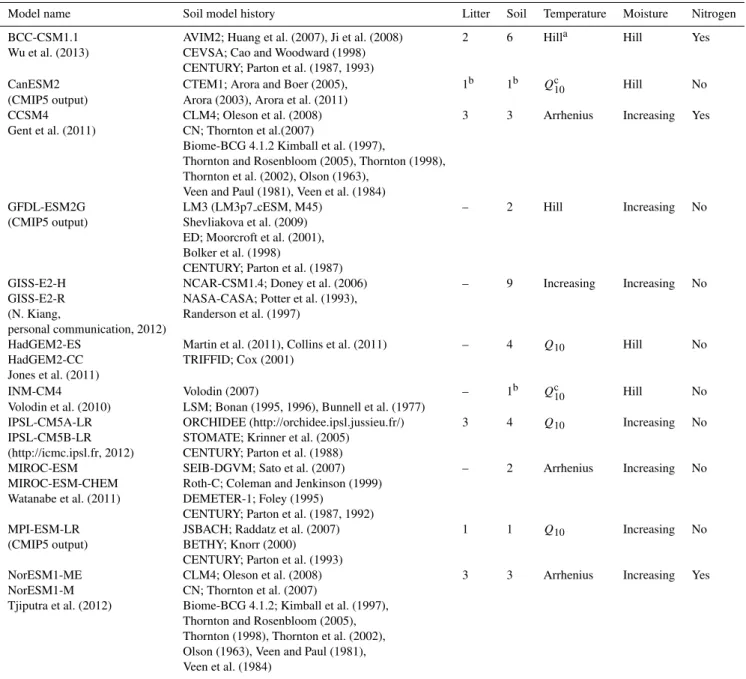
Table 1.Summary of soil carbon models including Earth system model names, history of model development, number of litter and soil pools, temperature and moisture functions, and representation of nitrogen cycling.

Model name Soil model history Litter Soil Temperature Moisture Nitrogen

BCC-CSM1.1 AVIM2; Huang et al. (2007), Ji et al. (2008) 2 6 Hilla Hill Yes Wu et al. (2013) CEVSA; Cao and Woodward (1998)

CENTURY; Parton et al. (1987, 1993)

CanESM2 CTEM1; Arora and Boer (2005), 1b 1b Qc₁₀ Hill No

(CMIP5 output) Arora (2003), Arora et al. (2011)

CCSM4 CLM4; Oleson et al. (2008) 3 3 Arrhenius Increasing Yes

Gent et al. (2011) CN; Thornton et al.(2007)

Biome-BCG 4.1.2 Kimball et al. (1997),

Thornton and Rosenbloom (2005), Thornton (1998), Thornton et al. (2002), Olson (1963),

Veen and Paul (1981), Veen et al. (1984)

GFDL-ESM2G LM3 (LM3p7 cESM, M45) – 2 Hill Increasing No

(CMIP5 output) Shevliakova et al. (2009) ED; Moorcroft et al. (2001), Bolker et al. (1998)

CENTURY; Parton et al. (1987)

GISS-E2-H NCAR-CSM1.4; Doney et al. (2006) – 9 Increasing Increasing No

GISS-E2-R NASA-CASA; Potter et al. (1993), (N. Kiang, Randerson et al. (1997)

personal communication, 2012)

HadGEM2-ES Martin et al. (2011), Collins et al. (2011) – 4 Q10 Hill No

HadGEM2-CC TRIFFID; Cox (2001) Jones et al. (2011)

INM-CM4 Volodin (2007) – 1b Qc₁₀ Hill No

Volodin et al. (2010) LSM; Bonan (1995, 1996), Bunnell et al. (1977)

IPSL-CM5A-LR ORCHIDEE (http://orchidee.ipsl.jussieu.fr/) 3 4 Q10 Increasing No

IPSL-CM5B-LR STOMATE; Krinner et al. (2005) (http://icmc.ipsl.fr, 2012) CENTURY; Parton et al. (1988)

MIROC-ESM SEIB-DGVM; Sato et al. (2007) – 2 Arrhenius Increasing No

MIROC-ESM-CHEM Roth-C; Coleman and Jenkinson (1999) Watanabe et al. (2011) DEMETER-1; Foley (1995)

CENTURY; Parton et al. (1987, 1992)

MPI-ESM-LR JSBACH; Raddatz et al. (2007) 1 1 Q10 Increasing No

(CMIP5 output) BETHY; Knorr (2000) CENTURY; Parton et al. (1993)

NorESM1-ME CLM4; Oleson et al. (2008) 3 3 Arrhenius Increasing Yes

NorESM1-M CN; Thornton et al. (2007)

Tjiputra et al. (2012) Biome-BCG 4.1.2; Kimball et al. (1997), Thornton and Rosenbloom (2005), Thornton (1998), Thornton et al. (2002), Olson (1963), Veen and Paul (1981), Veen et al. (1984)

a_{We define a hill function as a function that increases to a maximum and then decreases.}b_{Turnover parameterization dependent on biome or vegetation type.}c_Q 10value dependent on temperature.

of temperature (T) relative to a baseline (T0), such that

f (T )=Q(T₁₀−T0)/10. In this equation theQ10value is often set to between 1.5 and 2.5 based on estimates inferred from ecosystem flux measurements (Mahecha et al., 2010; Raich and Schlesinger, 1992) or the annual cycle of atmospheric CO2(Kaminski et al., 2002; Randerson et al., 2002). In some of the models, the temperature sensitivity of decomposition follows neither a Q10 nor Arrhenius relationship. For ex-ample, in BCC-CSM1.1 and GFDL-ESM2G, decomposition rate increases up to some optimal temperature and then

de-creases (Ji et al., 2008; Parton et al., 1987; Shevliakova et al., 2009). For the GISS-E2 model, the soil respiration re-sponse to temperature is a linear fit to data from Del Grosso et al. (2005) up to 30◦_{C, with a plateau above 30}◦_{C. In all}

We downloaded soil organic carbon, litter carbon, annual NPP, 2 m air temperature, soil temperature, and total soil wa-ter from thehistoricalsimulation, where available, for each ESM (cSoil, cLitter, npp, tas, tsl, and mrso, respectively, from the CMIP5 variable list). The monthly means for all variables from 1995–2005 were averaged for each grid cell to generate an overall mean for comparison to the HWSD and to use as drivers for our reduced complexity models (see be-low). We combined litter and soil carbon for our analysis and refer to the sum as soil carbon. Coarse woody debris (cCwd

from the variable list) was not included in the sum since there is no respiration from this pool in the two models that report it (CCSM4 and NorESM1). Global turnover times for soil carbon were calculated by dividing total soil carbon by to-tal terrestrial NPP from each ESM. INM-CM4 did not report NPP directly, so we derived NPP from gross primary produc-tion and autotrophic respiraproduc-tion (gppandrafrom the variable list). Soil temperatures were reported for each soil layer, but only the top 10 cm mean was used in this analysis. Land area was calculated from the grid area modified by the land cover for each model (areacellaandsftlf from the variable list, re-spectively). All ensemble members were averaged for each model; however, not all variables were available for each en-semble member. For example, GISS-E2-R reportedcSoilbut nottslfor ensemble member r1i1p1 at the time of download. We performed a hierarchical cluster analysis and found that ESMs from the same climate center generated very sim-ilar distributions of soil carbon for 1995–2005 (see Supple-ment Fig. S1). Clusters were constructed using complete linkage of the Euclidian distances between the global 1◦

-gridded soil carbon distributions for each model. Models from the same climate center always showed more than 90 % relative similarity and included the following pairs: GISS-E2 H and R, HadGEM2 ES and CC, IPSL-CM5 (LR) A and B, MIROC-ESM and MIROC-ESM-CHEM, and finally NorESM1 ME and M. As a result, these model pairs were averaged. We were left with 11 independent simulations, one representing each modeling center, that were evaluated using the approaches described below.

ESMs do not report the depth of carbon in the soil pro-file to CMIP5, making direct comparison with empirical es-timates of soil carbon difficult. Although many soil models were originally constructed to represent C dynamics at an ap-proximate depth range of 0 to 20 cm (e.g., Kelly et al., 1997), we assumed that all simulated soil carbon was contained within the top 1 m to simplify comparison with data sets. We recommend that future model intercomparison projects request soil carbon output from model simulations with spe-cific depth ranges (for example, soil carbon above 1 m and below 1 m) to allow for more accurate and direct comparison to survey data.

Fig. 1. Carbon density [kg m−2] in the top 1 m of soil from the Northern Circumpolar Soil Carbon Database (NCSCD) (Tarnocai et al., 2009) and Harmonized World Soil Database (HWSD) (FAO/IIASA/ISRIC/ISSCAS/JRC, 2012).

2.2 Data sets

2.2.1 Soil carbon

The HWSD provided empirical estimates of global soil carbon stocks to validate ESM simulations. The HWSD is a product of the Food and Agriculture Organization of the United Nations and the Land Use Change and Agri-culture Program of the International Institute for Applied Systems Analysis. The HWSD aggregates data from the European Soil Database (ESDB, 2004), the Soil Map of China (Shi et al., 2004), regional soil and terrain databases (Sombroek, 1984), and the FAO-UNESCO Soil Map of the World (FAO/UNESCO, 1981). Soil carbon stocks were calculated from bulk densities and organic carbon con-centrations given in the HWSD for the top 1 m of soil at a 0.5◦_×0.5◦ _{resolution (Fig. 1). Bulk density}

esti-mates in the HWSD were derived from soil texture; how-ever, this approach is not appropriate for high carbon soils (FAO/IIASA/ISRIC/ISSCAS/JRC, 2012; Saxton et al., 1986). Therefore, we replaced Histosol and Andisol bulk densities with values from the World Inventory of Soil Emis-sion Potentials (Batjes, 1996).

of soil (Fig. 1). The spatial and soil data used to develop this database were collected during the last 60 yr and originated from a variety of sources.

Quantitative uncertainty analyses for the HWSD and NC-SCD have not been performed and would be a challenge to construct because of the diverse data sources involved. How-ever, some estimate of uncertainty was essential to enable quantitative comparisons with the CMIP5 models. To gen-erate such a range for total soil carbon from both data sets, we constructed preliminary 95 % confidence intervals (CI95) using a qualitative approach. These estimates must be intpreted with caution because they are not based on formal er-ror propagation methods. Furthermore, these estimates only apply to database totals, and uncertainties for individual grid cells are likely to be larger.

For the HWSD, the major sources of error were related to analytical measurement of soil carbon, variation in car-bon content within a soil type, and mapping of soil types. Analytical measurements of soil carbon concentrations are generally precise, but measurements of soil bulk density are more uncertain and may contribute to CI95 values that are

±15 % of the mean carbon content for a given soil profile. Soil types in the HWSD are defined based on Food and Agri-culture Organization soil taxonomic units that are assumed to experience similar histories of soil forming factors such as climate, vegetation, disturbance, topography, and parent ma-terial. Batjes (1997) reported quartiles of soil carbon content for 23 soil taxonomic units based on 18 to 1270 soil profiles per unit. These quartiles suggest that soil carbon content is approximately log-normally distributed, allowing for calcu-lation of CI95values for each soil unit following log transfor-mation. When back transformed, CI95ranged from 6 to 33 % below the median to 6 to 48 % above the median, with an av-erage CI95 of 14 % below to 17 % above the median across all 23 units.

Another major source of HWSD uncertainty was related to the mapping of soil units and scaling of soil maps to 0.5◦_{. Soil taxonomic units and associated carbon contents}

were spatially extrapolated using expert knowledge informed by topography, geology, and vegetation (usually based on aerial photography). Original soil maps were scaled up in the HWSD by classifying each 0.5◦ _{grid cell according to}

its dominant soil unit. We assumed that the uncertainty as-sociated with mapping and scaling was similar in magnitude to measurement error and spatial variation, with a CI95 of approximately ±15 % of the mean. To estimate an overall CI95for the HWSD, we assumed that variation in soil carbon content within soil taxonomic units already included analyt-ical error, and that median carbon content within a soil unit is extrapolated by multiplying by the area of the unit. Thus the CI95values representing variation in soil carbon content and mapping uncertainty were summed to yield an overall CI95of 29 % below the mean to 32 % above the mean, or a range of 890 to 1660 Pg C with a mean of 1260 Pg C. This es-timate is broadly consistent with other empirical eses-timates of

global soil carbon (Eswaran et al., 1993; Jobbagy and Jack-son, 2000; Sombroek et al., 1993).

For the NCSCD, the uncertainties varied by geographic re-gion. The North American portion of the data set was based on analysis of 1169 pedons producing a medium to high con-fidence rating (66–80 %). Thus we estimated the CI95for the North American portion of the NCSCD to be 165±17 Pg C, corresponding to±10 % of the mean. In Eurasia, soil car-bon estimates were based on fewer pedons (591) plus 90 peat cores, producing a low to medium confidence rating (33–66 %). Therefore we estimated the CI95for the Eurasian region to be 331±99 Pg C, or ±30 % of the mean. Car-bon in Yedoma deposits and river deltas was estimated inde-pendently using surveyed depth information where available. This deeper soil carbon had the lowest confidence rating but contributed only∼1 % or 5 Pg of the database total; there-fore we allowed for a CI95 of 5±5 Pg C on this estimate. Together, these uncertainty estimates yielded an overall CI95 of roughly 500±120 Pg C for the first meter of soil.

2.2.2 Net primary productivity and temperature

To assess model skill in simulating key driving variables that could affect soil carbon stocks, we compared ESM outputs to temperature data from the Climate Research Unit (CRU) and to NPP data from a literature synthesis and from the Moderate Resolution Imaging Spectrometer (MODIS). The CRU and MODIS data also were used in parameter estima-tion for the reduced complexity models (Eqs. 1–2) to explain the spatial variation in observed global soil carbon with ob-served temperature and NPP. We used a 0.5◦_×0.5◦_gridded

air temperature data set from the CRU, specifically the 1995– 2005 mean of the tmp variable from CRU TS 3.10 (Jones and Harris, 2008). For NPP, we used the 0.008◦_×0.008◦

gridded MODIS product MOD17A3 from 2000–2011 (Zhao and Running, 2010). We also compared ESM-simulated NPP to Ito’s (2011) value of 54±11 Pg C yr−1 _{(mean ±} stan-dard deviation). This estimate was based on empirical models that used environmental parameters to extrapolate field mea-surements of NPP to the global scale. We considered ESM-simulated NPP values to be consistent with empirical data if they fell within 2 standard deviations of Ito’s (2011) estimate.

2.2.3 Biome map

To evaluate ESM soil carbon across biomes, we aggre-gated HWSD estimates and model simulations of soil carbon within biomes. The biome map was based on the MODIS land cover product MCD12C1 (Friedl et al., 2010; NASA LP DAAC, 2008) (Fig. S2). We assigned one of 16 land cover types to each 1◦_×1◦_{grid cell by taking the most common}

land cover from the original underlying 0.05◦_×0.05◦ _data.

Each 1◦_×1◦_{grid cell was assigned to one of 9 biomes:}

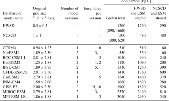
Table 2.Soil carbon totals across all grid cells in each ESM, grid cells present in the HWSD and ESM, and grid cells present in the NCSCD and ESM. Database totals include 95 % confidence intervals based on qualitative uncertainty analysis, shown in brackets. Values are rounded to the nearest 10 Pg C.

Soil carbon [Pg C]

Original Number of Ensembles HWSD NCSCD

Database or grid size model per and ESM and ESM

model name ◦lat.×◦long. versions version Global total shared shared

HWSD 0.5×_{0.5 – – 1260 1260 290}

[890, 1660]

NCSCD 1×1 – – 500 480 480

[380, 620]

CCSM4 0.94×1.25 1 6 510 510 60

NorESM1 1.89×2.50 2 3, 1 550 530 60

BCC-CSM1.1 2.81×2.81 1 3 1050 990 240

HadGEM2 1.25×1.88 2 1, 2 1120 1090 200

IPSL-CM5 1.89×3.75 2 5, 1 1310 1250 390

GFDL-ESM2G 2.01×2.50 1 1 1410 1360 690

CanESM2 2.79×2.81 1 5 1540 1460 370

INM-CM4 1.50×_{2.00 1 1 1680 1630 280}

GISS-E2 2.00×2.50 2 15, 16 1900 1820 520

MIROC-ESM 2.79×2.81 2 3, 1 2570 2490 810

MPI-ESM-LR 1.86×1.88 1 3 3040 2930 340

snow and ice, or permanent wetland. Details for the biome construction can be found in Fig. S2 in the Supplement.

2.3 Regridding approach

All model outputs and data sets were regridded to 1◦_×1◦_for

biome- and grid-scale comparisons. Our regridding approach assumed conservation of mass and that a latitudinal degree is proportional to distance for close grid cells. Regridding the outputs to 1◦_×1◦ _{downscaled the models while upscaling}

the data (Table 2).

2.4 Assessing driving variables for soil C stocks

We developed several reduced complexity models to evalu-ate the drivers of simulevalu-ated soil carbon variability and facil-itate comparisons between ESMs. These reduced complex-ity models consisted of a single pool of soil carbon at each grid cell driven by locally varying NPP, soil temperature, and soil moisture (Figs. S3, S4, S5 in Supplement) and globally uniform parameters including a decomposition rate constant,

Q10 value, and moisture coefficient. By applying the same simple model, we were able to compare parameters across ESMs and assess which variables had the strongest control over soil carbon. Driving variables for the reduced complex-ity models were taken from ESM annual means of NPP, soil temperature (T, top 10 cm mean), and total soil water content (W) over the period 1995–2005.

Our reduced complexity models assumed that the soil car-bon pool (C) in grid celliwas at steady state, such that NPP

inputs equaled outputs from heterotrophic respiration (R): 0=dCi

dt =NPPi−Ri.

Carbon pools were not expected to be exactly at steady state for 1995–2005, and mean grid differences be-tween NPP and R across the ESMs ranged from 0.01 to 0.12 kg m−2_yr−1_{, or between 1 % and 20 % of the mean grid} NPP for this period. Thus the ESMs were close to steady state, and we assumed steady state to simplify our analysis. For the simplest reduced complexity model, we assumed that soil heterotrophic respiration was directly proportional to the soil carbon pool with a spatially uniform decomposition rate constantk(Olson, 1963; Parton et al., 1987):

Ri =kCi.

Combining the two above equations yielded the simplest reduced complexity model, Eq. (1), in which soil carbon was proportional to NPP and inversely proportional to a global decomposition rate (k):

Ci= NPPi

k . (1)

We formulated a second reduced complexity model, Eq. 2, in which soil respiration in each grid cell also depended on soil temperature (T )according to aQ10 function with a baseline temperature of 15◦_{C (Lloyd and Taylor, 1994):} Ci=

NPPi

kQ(Ti−15)/10

10

A third reduced complexity model, Eq. (3), included a mois-ture modifier that increased with total soil water content (Wi) normalized to maximal soil water content for each ESM (Wx) according to an exponential function, wherebwas a positive scaling exponent:

Ci=

NPPi

kQ(Ti−15)/10

10

Wi

Wx

b. (3)

The parametersk, Q10, andb in each reduced complex-ity model were optimized using ESM soil carbon and driv-ing variables across all grid cells. We used a constrained Broyden–Fletcher–Goldfarb–Shanno optimization algorithm (Byrd et al., 1995), a quasi-Newtonian method, as imple-mented in R 2.13.1 (R Development Core Team, 2012). This algorithm was selected for parameter fitting because of its ro-bust convergence and short run time. We ran the optimization with the following constraints:k∈ 10−4_,10

, Q10∈(1,4), andb∈(0,3). The initial parameter estimates werek=0.1,

Q10=1, and b=0. We used the root mean square error (RMSE) as the measure function. The optimization was per-formed only on grid cells with non-zero soil carbon values.

We conducted an additional analysis to assess the causes of variation in simulated soil carbon across ESMs (Eqs. 4– 7). For this analysis, we used a modified version of Eq. (2) to predict total global soil carbon (C)for each ESM:

C=X

i

NPPi

kQ(Ti−15)/10

10

, (4)

where theQ10 andk parameters were derived from fitting Eq. (2) to the spatial distribution of soil carbon (at 1◦

reso-lution) from each ESM as described above. Grid-scale NPP outputs (NPPi)and soil temperatures (Ti)from each ESM were used as drivers in Eq. (4) to calculate soil carbon in each grid cell i. Soil carbon was then summed across all grid cells in each ESM to calculate the global soil carbon pool (C). Thus Eq. (4) represents the contribution of both model parameterization (Q10andk) and soil carbon drivers (NPPi andTi)to the global soil carbon pool. To isolate the effect of ESM parameterization onC, we substituted multi-model mean values for NPP (NPPi)and temperature (T¯i)into Eq. (4) for each grid celli:

C=X

i

NPPi

kQ(T¯i−15)/10

10

. (5)

To isolate the effect of ESM driving variables onC, we substituted multi-model mean values for Q10 (Q¯10)and k (_k)¯ _{into Eq. (4):}

C=X

i

NPPi

¯

kQ¯(T₁₀i−15)/10

. (6)

Finally, we substituted only the multi-model mean tempera-ture into Eq. (4) to isolate the effect of NPP on inter-model variation inC:

C=X

i

NPPi

kQ(T¯i−15)/10

10

. (7)

Using regression analysis, we compared the predictedC

from Eqs. (4)–(7) to the totals simulated by the ESMs. These regressions measure the contribution of parameteriza-tion (Eq. 5) versus driving variables (Eqs. 6 and 7) to varia-tion in soil carbon totals across ESMs. We excluded GISS-E2 from this inter-model analysis because Eq. (2) could not be fit to this model, and thereforeQ₁₀andkwere not available.

2.5 Statistical analyses

ESM simulations were compared to data sets using Pear-son correlation coefficients, RMSE, and Taylor scores in R 2.13.1 (R Development Core Team, 2012). The Tay-lor score (TS)combines the Pearson correlation coefficient (r) and standard deviation (σ ) of the model results (m) compared to the data (d):

TS(d, m)=

4 [1+r (d, m)]

h_{σ ( m)}

σ (d) + σ (d) σ ( m)

i2

[1+rmax]

,

wherermaxis the maximum correlation attainable, assumed to be 1 in this case (Taylor, 2001). Biome-aggregated totals were compared to observations using linear regression.

3 Results

3.1 Global soil carbon stocks and turnover times

The mean (±SD) global soil carbon reported across all ESMs was 1520±770 Pg, whereas the global soil carbon in the HWSD was 1260 Pg with a CI95of 890 to 1660 Pg (Table 2, Fig. 2). CCSM4 reported the lowest total at 510 Pg C and MPI-ESM-LR the highest at 3040 Pg C. Examining only the area shared by all ESMs and the HWSD reduces the global carbon totals but does not substantially change the rank or-der of the models (Table 2). CCSM4 and NorESM1 unor-der- under-estimated global soil carbon stocks by about 50 %, whereas GISS-E2, MIROC-ESM, and MPI-ESM-LR overestimated global soil carbon stocks anywhere from 50 % to 140 %. The other models predicted global soil carbon totals that were within 35 % of the HWSD global mean and fell within its preliminary CI95.

Fig. 2.Global soil carbon (top), net primary production (middle), and soil carbon turnover times (bottom) for observations and ESMs. Turnover times were calculated as HWSD carbon divided by MODIS NPP for the observations, and simulated global soil carbon divided by simulated global NPP for the ESMs. The gray hashed area on the top panel represents the 95 % confidence interval for global soil carbon

in the HWSD based on a qualitative uncertainty analysis (see text). The hashed area on the middle panel represents±2 standard deviations

around the mean global NPP estimate from Ito (2011) based on empirical models. The hashed area on the bottom panel indicates the range of turnover times for global soil carbon found in the literature (Amundson, 2001; Raich and Schlesinger, 1992). For soil carbon and NPP, each global estimate is separated into individual biome components according to the legend shown in the top panel.

observed in the NCSCD. HadGEM2, BCC-CSM1.1, INM-CM4, MPI-ESM, and CanESM2 also simulated soil carbon totals below the preliminary CI95 for the NCSCD. In con-trast, GFDL-ESM2G and MIROC-ESM overestimated high latitude soil carbon stocks by 45–60 %. Only IPSL-CM5 and GISS-E2 soil carbon fell within the CI95for the NCSCD.

Variation in global soil carbon stocks simulated by ESMs could be driven by variation in modeled NPP, and we found that global terrestrial NPP varied by a factor of 2.6 across the models (Fig. 2). CCSM4, BCC-CSM1.1, CanESM2,

INM-CM4, GISS-E2, and MIROC-ESM all predicted global NPP values within 2 standard deviations of the Ito (2011) estimate of 54 Pg C yr−1_{, ranging from 46 to 73 Pg C yr}−1_{, whereas} the remaining 5 models fell outside this range. NPP from MODIS was similar to Ito (2011) at 52 Pg C yr−1_{. At high} northern latitudes, NPP estimates from the ESMs were more variable (1.7 to 10.1 Pg C yr−1), compared to a MODIS esti-mate of 4.7 Pg C yr−1_{(Fig. S6 in Supplement).}

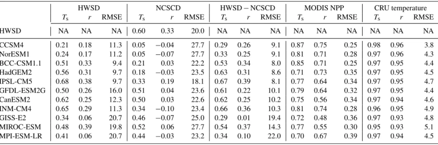
Table 3.Goodness-of-fit measures by grid cell for each ESM including soil carbon versus the HWSD, soil carbon versus NCSCD, soil carbon

versus HWSD without NCSCD grid cells (HWSD−NCSCD), NPP versus MODIS NPP, and land 2 m air surface temperature versus CRU

2 m air temperature.T_S=_{Taylor score;}r=_{Pearson correlation coefficient; RMSE}=_{root mean square error. RMSE has units of kg C m}−2

for the soil carbon comparisons, kg C m−2yr−1for NPP, and◦C for temperature.

HWSD NCSCD HWSD−NCSCD MODIS NPP CRU temperature

Ts r RMSE Ts r RMSE Ts r RMSE Ts r RMSE Ts r RMSE

HWSD NA NA NA 0.60 0.33 20.0 NA NA NA NA NA NA NA NA NA

CCSM4 0.21 0.18 11.3 0.05 −0.04 27.7 0.29 0.26 9.1 0.87 0.75 0.25 0.98 0.96 3.8 NorESM1 0.24 0.17 11.2 0.05 −0.07 27.7 0.33 0.25 9.1 0.81 0.71 0.28 0.97 0.96 4.3 BCC-CSM1.1 0.51 0.33 9.4 0.21 0.03 22.2 0.53 0.34 8.0 0.85 0.71 0.25 0.97 0.95 4.4 HadGEM2 0.56 0.31 9.7 0.18 −0.03 23.5 0.63 0.31 8.6 0.71 0.73 0.35 0.97 0.95 4.5 IPSL-CM5 0.68 0.38 9.7 0.33 0.19 18.1 0.67 0.39 8.1 0.77 0.64 0.34 0.97 0.95 4.7 GFDL-ESM2G 0.50 0.26 16.0 0.51 0.04 23.6 0.61 0.22 10.1 0.79 0.64 0.32 0.97 0.95 4.4 CanESM2 0.62 0.25 12.3 0.50 0.03 22.6 0.62 0.25 10.2 0.75 0.56 0.34 0.97 0.94 4.6 INM-CM4 0.65 0.29 11.3 0.34 −0.10 23.4 0.66 0.36 10.3 0.81 0.74 0.28 0.96 0.95 4.9 GISS-E2 0.34 0.06 20.7 0.46 −0.07 25.0 0.29 0.01 19.4 0.72 0.48 0.36 0.97 0.93 4.8 MIROC-ESM 0.48 0.39 19.8 0.52 0.06 27.7 0.54 0.37 14.3 0.77 0.55 0.30 0.95 0.93 5.1 MPI-ESM-LR 0.41 0.06 20.7 0.44 −0.03 23.2 0.34 0.10 22.0 0.70 0.67 0.39 0.97 0.94 4.5

stocks and NPP estimates from each model (Fig. 2). Using MODIS NPP, we calculated a turnover time of 24 yr for soil carbon in the HWSD. This estimate is consistent with the range of 18 to 32 yr reported in other studies (Amundson, 2001; Raich and Schlesinger, 1992). However, CanESM2 and INM-CM4 were the only two ESMs with turnover times that also fell within this range (Fig. 2). At high northern lat-itudes, 5 of the 11 models had turnover times that were con-siderably lower than the observations, whereas only 2 of the models had turnover times exceeding observational estimates (Fig. S6 see Supplement). Turnover times for high northern latitudes were 101.2 yr for the NCSCD and 60.8 yr for the HWSD.

3.2 Spatial distribution of soil carbon

The spatial distribution of soil carbon stocks varied widely among the ESMs (Fig. 3). CCSM4 and NorESM1 had the lowest overall soil carbon densities, but showed relatively high densities in northern South America, central Africa, eastern Asia, and eastern North America. HadGEM2, BCC-CSM1.1, and INM-CM4 showed a broader range of soil car-bon densities with high densities in North America, western South America, central Africa, Southeast Asia, and north-central Eurasia. HadGEM2 also showed elevated soil carbon in southeastern South America. CanESM2 predicted high soil carbon in northeastern North America, northern Europe, northeastern Asia, central Africa, and eastern South America. GFDL-ESM2G and MIROC-ESM showed uniformly high carbon densities across all high northern latitudes and around the Tibetan Plateau. GISS-E2 predicted a region of high soil carbon across the northern latitudes of North America and Europe, as well as another area of high soil carbon from northeastern to southwestern Asia. MPI-ESM-LR showed an inverse pattern compared with the other ESMs; soil

car-bon peaked in the mid-latitudes across Asia, western North America, eastern Africa, southern South America, and south-ern coastal Australia.

There was generally poor agreement between the ESMs and the HWSD soil carbon distribution at the 1◦_scale

(Ta-ble 3). Compared to the HWSD, ESMs had Pearson correla-tion coefficients between 0.06 and 0.39, RMSE between 9.4 and 20.7 kg C m−2_{, and Taylor scores ranging from 0.21 to} 0.68. Omitting the high latitude portion of the HWSD that overlapped with the NCSCD modestly improved these per-formance metrics for most but not all ESMs (Table 3). Model agreement with NCSCD soil carbon was poor with Pearson correlation coefficients between−0.10 and 0.19, RMSE be-tween 18.0 and 27.7 kg C m−2_{, and Taylor scores between} 0.05 and 0.52. Agreement between the HWSD and NCSCD also was also low in the areas where the two data sets over-lapped (Pearson correlation coefficient of 0.33, RMSE of 20.0 kg C m−2_{, and Taylor score of 0.60), although better} than the agreement between any individual ESM and the NC-SCD.

ESM agreement with the HWSD generally improved at the biome level (Fig. 4). BCC-CSM1.1 and CanESM2 stood out as being highly correlated with the HWSD (R2>0.90,

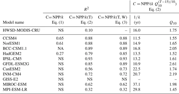
Table 4.Coefficients of determination (R2)and global-scale parameters (1/ k andQ10)from reduced complexity models of ESM soil

carbon distributions. Eq. (1): dependence on NPP; Eq. (2): dependence on NPP and soil temperature; Eq. (3): dependence on NPP, soil

temperature, and soil moisture. Parameters are shown from Eq. (2) with 1/ kanalogous to turnover time. HWSD-MODIS-CRU represents

reduced complexity models based on observational data. The reduced complexity model for CanESM2 was the only one improved by

including soil moisture and had a turnover time (1/ k) of 8.20 yr,Q₁₀of 1.48, and moisture exponent of 0.46 based on Eq. (3). AllR2values

were statistically significant (R2>0.05,p <0.01)unless otherwise indicated (NS).

C=NPP/(k Q(T₁₀−15)/10)

R2 Eq. (2)

C=NPP/k C=NPP/k(T) C=NPP/k(T, W) 1/ k

Model name Eq. (1) Eq. (2) Eq. (3) (yr) Q10

HWSD-MODIS-CRU NS 0.10 – 16.0 1.75

CCSM4 0.65 0.88 0.88 11.5 1.55

NorESM1 0.61 0.88 0.88 14.9 1.65

BCC-CSM1.1 NA 0.89 0.89 16.8 2.05

HadGEM2 0.27 0.79 0.85 13.5 1.52

IPSL-CM5 NS 0.93 0.93 13.2 1.61

GFDL-ESM2G NS 0.85 0.89 10.9 2.61

CanESM2 NS 0.56 0.73 22.5 1.74

INM-CM4 NS 0.72 0.72 20.7 2.19

GISS-E2 NS NS NS – –

MIROC-ESM NS 0.62 0.62 37.1 1.98

MPI-ESM-LR NS 0.32 0.32 29.8 1.45

correlated with the HWSD (0.70> R2>0.65,p <0.01), but consistently underestimated biome totals particularly in tun-dra, boreal forest, and desert and shrubland. Biome totals from MPI-ESM-LR were also moderately correlated with the HWSD (R2=0.62, p <0.01), but this model overes-timated most biome totals, particularly grasslands and sa-vanna. GFDL-ESM2G and GISS-E2 were weak to moder-ately correlated with the HWSD on the biome level (R2=

0.38 and R2=0.51, respectively). GFDL-ESM2G overes-timated biome totals from tundra and boreal forests while underestimating the other biomes. GISS-E2 overestimated biome totals in desert and shrublands, grasslands and sa-vanna, tundra, and boreal forests while underestimating trop-ical rainforests.

3.3 Drivers of soil carbon distributions and global stocks

The spatial variability in 8 of the 11 ESMs was well ex-plained by the reduced complexity model driven by NPP and soil temperature (Eq. 2) with R2 values between 0.72 and 0.93 (Table 4). Consistent with our global-scale calcula-tions (Fig. 2), the turnover times (1/ k) for global soil carbon inferred from Eq. (2) (at a baseline temperature of 15◦_C)

varied from 11 to 37 yr, andQ10 values ranged from 1.5 to 2.6 (Table 4). The reduced complexity model for CanESM2 was the only one significantly improved by the addition of soil moisture (Eq. 3), with theR2value increasing from 0.56 to 0.73. Soil carbon outputs from GISS-E2 (R2<0.01) and

MPI-ESM-LR (R2=0.32) were not well explained by any of the reduced complexity models.

Given the strong relationships between soil carbon, tem-perature, and NPP illustrated by our reduced complexity models, model skill in simulating driving variables could strongly influence simulated soil carbon stocks (Table 3). ESMs varied in their ability to capture the observed 1◦_spatial

distribution of NPP (Pearson correlation coefficients from 0.48 to 0.75, biome regressionR2values from 0.86 to 0.99; Table 3, Fig. S7 in the Supplement). In contrast, models performed better at simulating surface air temperature ob-servations (correlations from 0.93 to 0.96, biome regression

R2 values from 0.93 to 0.97; Fig. S8 in the Supplement). Although air temperature is not directly comparable to soil temperature, particularly in areas with thick organic soils, the biome level correlation between soil and air tempera-ture was high across all ESMs (R2values higher than 0.97; Fig. S9). INM-CM4, GISS-E2, BCC-CSM1.1, CCSM4, and NorESM1 all showed warmer soil temperatures compared to air temperatures in northern biomes (Fig. S9). In contrast to the strong relationships we found between soil carbon, NPP, and temperature in the ESMs, the 1◦ _spatial

distribu-tion of soil carbon from the HWSD was not well explained by MODIS NPP and CRU surface air temperature data using the same reduced complexity model (R2 value of 0.10 for Eq. (2); Table 4).

Fig. 3.Soil carbon densities [kg m−2] from Earth system models. These soil carbon densities represent 1995–2005 means from thehistorical

simulations of the Climate Model Intercomparison Project 5.

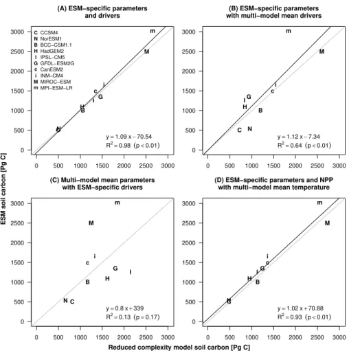
(Fig. 5). Reduced complexity models using ESM-specific values for k and Q₁₀ and ESM-derived driving variables were able to explain 98 % the variation in total soil carbon across ESMs (Fig. 5a). Most of the variation in soil carbon across ESMs could be attributed to differences in parameter-ization as represented by Eq. (5) (R2=0.64, Fig. 5b). There was no significant cross-ESM variation due to differences in driving variables alone as represented by Eq. (6) (Fig. 5c). However, driving variables must interact with parameters, since the variances explained by drivers alone (13 %, not sig-nificant) and parameters alone (64 %) did not sum to 98 % (Fig. 5a–c). NPP was likely the main driving variable in this interaction, since using the multi-model mean temperature at each grid cell (Eq. 7) still allowed us to explain 93 % of the variation in global soil carbon across ESMs (Fig. 5d).

4 Discussion

0 50 100 150 200 250 0 50 100 150 200 250 CCSM4 ● ● ● ● ● ● ● ● y=0.46 x−6.3 R2=0.68 (p<0.01)

0 50 100 150 200 250 0 50 100 150 200 250 NorESM1 ● ● ● ● ● ● ● ● y=0.48 x−4.6 R2=0.69 (p<0.01)

0 50 100 150 200 250 0 50 100 150 200 250 BCC−CSM1.1 ● ● ● ● ● ● ● ● y=0.86 x−2.66 R2=0.95 (p<0.01)

0 50 100 150 200 250 300 0 50 100 150 200 250 300 HadGEM2 ● ● ● ● ● ● ● ● y=0.99 x−11.48 R2=0.88 (p<0.01)

0 50 100 150 200 250 0 50 100 150 200 250 IPSL−CM5 ● ● ● ● ● ● ● ●

y=1.05 x−0.22 R2=0.85 (p<0.01)

0 100 200 300 400 0 100 200 300 400 GFDL−ESM2G ● ● ● ● ● ● ● ● y=1.04 x+9.77 R2=0.38 (p=0.03)

0 100 200 300 0 100 200 300 CanESM2 ● ● ● ● ● ● ● ●

y=1.28 x−6.25 R2=0.91 (p<0.01)

0 100 200 300 400 500 0 100 200 300 400 500 INM−CM4 ● ● ● ● ● ● ● ●

y=1.53 x−21.68 R2=0.87 (p<0.01)

0 100 200 300 400 0 100 200 300 400 GISS−E2 ● ● ● ● ● ● ● ●

y=1.4 x+13.94 R2=0.51 (p<0.01)

0 100 200 300 400 500 600 0 100 200 300 400 500 600 MIROC−ESM ● ● ● ● ● ● ● ●

y=2.11 x−7.66 R2=0.87 (p<0.01)

0 200 400 600 800 1000 0 200 400 600 800 1000 MPI−ESM−LR ● ● ● ● ● ● ● ●

y=2.91 x−55.87 R2=0.62 (p<0.01)

HWSD soil carbon [Pg C]

ESM soil carbon [Pg C]

● ● ● ● ● ● ● ● Permanent wetlands Tundra Boreal forest Temperate forest Grasslands and savanna Desert and shrublands Cropland and urban Tropical rainforest

Fig. 4.Linear regression of ESM versus HWSD soil carbon totals [Pg C] for the 8 major biomes. The gray line indicates a 1:1 relationship and the black line is the linear regression.

or parameterization of the decomposition response to driv-ing variables. Better performance at the global and biome scales may be due to aggregation of environmental variation that was not captured by the models at finer spatial scales. For instance, topographic controls on soil texture, moisture,

CN B H

I G c

i

M m

0 500 1000 1500 2000 2500 3000 0

500 1000 1500 2000 2500 3000

and drivers (A) ESM−specific parameters

C N B H I G c i M m

CCSM4 NorESM1 BCC−CSM1.1 HadGEM2 IPSL−CM5 GFDL−ESM2G CanESM2 INM−CM4 MIROC−ESM MPI−ESM−LR

y=1.09 x−70.54 R2=0.98 (p<0.01)

C N B H IG

c i

M m

0 500 1000 1500 2000 2500 3000 0

500 1000 1500 2000 2500 3000

with multi−model mean drivers (B) ESM−specific parameters

y=1.12 x−7.34 R2=0.64 (p<0.01)

C N

B H

I G c

i M

m

0 500 1000 1500 2000 2500 3000 0

500 1000 1500 2000 2500 3000

with ESM−specific drivers (C) Multi−model mean parameters

y=0.8 x+339 R2₌0.13 (p₌0.17)

C N

B H

IG c i

M m

0 500 1000 1500 2000 2500 3000 0

500 1000 1500 2000 2500 3000

with multi−model mean temperature (D) ESM−specific parameters and NPP

y=1.02 x+70.88 R2=0.93 (p_<0.01)

ESM soil carbon [Pg C]

Reduced complexity model soil carbon [Pg C]

Fig. 5.Relationship between global soil carbon totals from ESMs and global soil carbon totals predicted by reduced complexity models

(Eqs. 4–7). The reduced complexity model in(A)used ESM-specific parameters and drivers (Eq. 4);(B)used ESM-specific parameters with

multi-model mean NPP and soil temperature (Eq. 5);(C)used multi-model mean parameters and ESM-specific NPP and soil temperature

(Eq. 6);(D)used ESM specific parameters and NPP but multi-model mean soil temperature (Eq. 7). The gray line indicates a 1:1 fit and the

black line is the linear regression.

4.1 Data uncertainties

Our ability to evaluate model performance relies on high quality empirical data with associated estimates of uncer-tainty. Whether model simulations diverge from the data is difficult to assess without a formal analysis of uncertainty in the data. Despite their comprehensiveness, the HWSD and NCSCD lack quantitative uncertainty estimates, thereby con-straining our ability to use these data sets for benchmarking ESMs. Our preliminary analyses based on a qualitative as-sessment indicated that the uncertainty in empirical estimates of soil carbon stocks could exceed 770 Pg C at the global scale, an amount similar to the entire pool of atmospheric carbon.

At high northern latitudes, there was substantial disagree-ment between the two data sets. NCSCD estimates of CI95 were between 380 and 620 Pg C, whereas the corresponding HWSD estimate was only 290 Pg C. However, the HWSD did not include regional uncertainty information, meaning that

the two estimates may agree once a formal uncertainty anal-ysis has been performed. Such an analanal-ysis requires quantifi-cation of uncertainty in both measurement and scaling pro-cesses used to construct the spatial distribution of soil car-bon. Uncertainty in the measurement of soil properties such as bulk density and carbon concentration must be integrated with errors involved in extrapolating data from individual soil profiles to the regional scale. Detailed analysis of the accu-racy of soil maps will likely be essential for quantifying the uncertainty in this extrapolation process.

4.2 Driving variables

complexity models showed that differences in NPP con-tributed significantly to differences in soil carbon across ESMs (Fig. 5). NPP was also a significant driver of soil car-bon within ESMs (Table 3), suggesting it should be a focal variable for improving soil carbon estimates. Given the large range of global NPP across ESMs (Fig. 2) and the low Taylor scores observed for some models in comparison to MODIS NPP (Table 3), it may be possible to improve soil carbon simulations by revising photosynthesis and autotrophic res-piration algorithms in some of the ESMs so that NPP is more consistent with contemporary observations.

In contrast to NPP, differences in soil temperature did not contribute significantly to differences in soil carbon stocks across ESMs (Fig. 5). However, our reduced complexity models indicated that soil temperature was important for explaining soil carbon variation within models (Table 4). Therefore, simulation of soil temperature could also be a fo-cal area for model improvement, especially since other stud-ies suggest that soil temperature is not consistently well rep-resented in ESMs. For example, the physical coupling be-tween surface air temperature and soil temperature at high latitudes differs considerably across ESMs, which influences the spatial distribution of permafrost (Koven et al., 2012; Slater and Lawrence, 2013). Even if ESMs can simulate av-erage air temperatures consistent with observations (Table 3, Fig. S8), fine-scale differences in the ability to represent soil temperatures (Fig. S9) and permafrost could have con-sequences for soil carbon distributions.

Soil moisture did not play an important role as a driv-ing variable for soil carbon in our reduced complexity mod-els, indicating that for most models this variable did not strongly control spatial patterns in soil carbon stocks (Ta-ble 4) or differences among models (Fig. 5). This result was unexpected because soil moisture affects decomposition rates in all ESMs (Table 1). Furthermore, other studies have shown that soil carbon stocks depend on the response of het-erotrophic respiration to soil moisture in global models, al-though NPP and soil temperature were also important drivers of soil carbon (Falloon et al., 2011). It is possible that soil moisture influences soil carbon stocks in ESMs, but our re-duced complexity model was unable to statistically distin-guish the soil moisture effect from the NPP effect because these two drivers often covary.

Alternatively, the exponential form of the moisture func-tion in our reduced complexity model might have been inap-propriate if decomposition rates decline at high soil moisture. Based on empirical data, a substantial fraction of global soil carbon likely resides in areas where poor soil drainage im-pedes organic matter oxidation (Gorham, 1991). It is likely that the interaction of topographic controls and soil texture with soil moisture is not well represented in the current gen-eration of ESMs. New approaches may be needed to deter-mine which grid cells are poorly drained, and the rate at which organic soils form in these area (Ise et al., 2008). We also recommend that future CMIP archives require soil

mois-ture information for different soil layers to facilitate bench-marking studies on the response of carbon to moisture in the soil profile.

Although our reduced complexity models indicated that soil carbon simulated by ESMs was driven primarily by NPP and temperature, this relationship was much weaker with ob-servational data. According to the same reduced complex-ity model used for the ESMs, MODIS NPP and CRU sur-face air temperatures were only able to explain 10 % of the spatial variation in HWSD soil carbon stocks. Thus the variables that drive soil carbon stocks in ESMs may differ from those that determine observed carbon stocks. For ex-ample, soil temperatures in organic-rich soils may be weakly coupled to air temperatures (Koven et al., 2011; Slater and Lawrence, 2013), in contrast to the strong coupling predicted by most ESMs (Fig. S9). Alternatively, the mathematical form of our reduced complexity model may have been in-appropriate for the observational data, even though it was appropriate for most ESM outputs. Regardless, our results imply that ESMs may need to incorporate a broader range of environmental drivers and processes to improve model– data agreement. Even if simulations of NPP and soil temper-ature can be improved in ESMs, these drivers have a limited ability to explain spatial patterns in global soil carbon with current model structures.

4.3 Parameterization and model structure

We found that parameterization was a major source of varia-tion in ESM soil carbon simulavaria-tions (Fig. 5). In some of the ESMs such as CCSM4, soil carbon turnover may be too fast, whereas in other models such as MIROC-ESM, turnover may be too slow (Fig. 2). To address these issues, ESMs could use terrestrial radiocarbon observations (both the total in-ventory and vertical distribution of14_{C in different biomes)} to help constrain rates of soil carbon turnover (Torn et al., 1997; Trumbore, 2009). Another avenue of improvement for ESM parameterization could focus on processes that operate on fine spatial scales. Differences in soil texture and topog-raphy may lead to non-linear effects on soil carbon storage that are not well described by the average characteristics of a grid cell. For instance, relatively small-scale topographic variations are associated with peatland formation, and it is unclear how to scale these effects globally (Gorham, 1991; Koven et al., 2011). A multi-scale approach is required to determine which processes are important at the global scale and how to represent them.

the right reasons. For example, models with incorrect mech-anisms or drivers could be tuned to correctly simulate current soil carbon stocks, but might incorrectly simulate soil carbon stock changes in the future.

We initially hypothesized that models with more pools would have greater flexibility and capture more of the spa-tial variation in soil carbon. However, the structural fea-tures that we examined did not clearly relate to differences in ESM agreement with empirical data (Tables 1, 3). We saw no pattern in ESM-data agreement with respect to num-ber of soil carbon pools, temperature and moisture sensitiv-ity functions, or presence of a nitrogen component. Further-more, our reduced complexity model (Eq. 3) explained most of the spatial variation within 9 of 11 models (0.62< R2<

0.93). This result confirmed that, despite different simulated stocks of soil carbon, most of the models share a similar underlying structure. Such similarity means that the mod-els likely make similar assumptions about the mechanisms regulating soil carbon cycling. If these underlying assump-tions are incorrect or incomplete, the resulting errors will be present in all of the models.

CanESM2, MPI-ESM-LR, and GISS-E2 are three excep-tions that were not well explained by our reduced complexity model (Eq. 2) driven by NPP and soil temperature (Table 4), and thus may be examples of models with structural differ-ences. CanESM2 was the only model in which soil water content contributed to the explanatory power of the reduced complexity model (R2 value improved from 0.57 to 0.74). This dependency on soil water content may be partly ex-plained by the biome-specific turnover time in CanESM2. Since biomes are partially determined by precipitation and soil moisture status, biome-specific turnover times might have resulted in a tighter relationship between soil carbon and moisture in our reduced complexity model. Outputs from MPI-ESM-LR were only moderately explained by our re-duced complexity models (R2value 0.32). We do not have a good explanation for the poor fit since there was no signif-icant deviation in documented model structure, and driving variables were roughly in line with other model simulations. GISS-E2 outputs were not explained at all by the reduced complexity model (R2 value less than 0.01). Unlike other models, GISS-E2 showed a unique disconnect between NPP and soil carbon which could be due to differences in the way plant biomass is allocated to litter in the model. However, we cannot offer a definitive explanation for the poor fit.

All ESMs may be missing key processes governing long-term carbon storage that affect model–data agreement. De-composition models currently used in all ESMs are built on the assumption that carbon substrates have intrinsic chemi-cal decomposition rates (Parton et al., 1993). However, there is an emerging consensus that key abiotic and biotic factors have a stronger governing role in decomposition than the carbon compounds themselves (Schmidt et al., 2011). These key governing components may include aggregate interac-tions (Six et al., 2000), microbial dynamics (Todd-Brown et

al., 2012), cryoturbation (Koven et al., 2011), syngenetic soil formation (Fan et al., 2008; Shur et al., 2004), extra-cellular enzyme dynamics (German et al., 2011), and rare substrate formation (Allison, 2006). Representing these pro-cesses in the structure of soil carbon models remains a ma-jor challenge. However, smaller-scale decomposition mod-els have begun to explore several of these mechanisms (Manzoni and Porporato, 2009).

Recent advances in the theory of microbial decomposi-tion could provide a foundadecomposi-tion for major changes in the structure of soil carbon models used in ESMs. Schimel and Weintraub (2003) proposed a model in which decomposition was mediated by soil enzymes and microbial biomass. Later models expanded this framework to include microbial func-tional groups that preferentially decompose specific substrate types (Moorhead and Sinsabaugh, 2006). In contrast to cur-rent substrate pool models used in ESMs, biomass-mediated decomposition models would likely include non-linear pro-cesses such as Monod uptake or Michaelis–Menten enzyme kinetics. These non-linear effects could produce very dif-ferent behaviors at daily, annual, and centennial timescales. Compared to substrate pool models, models driven by mi-crobial biomass predict smaller losses of soil carbon under warming due to declines in microbial growth efficiency with higher temperature (Allison et al., 2010).

5 Conclusions

Overall, we found that some ESMs simulated soil carbon stocks consistent with empirical estimates at the global and biome scales. However, all of the models had difficulty rep-resenting soil carbon at the 1◦_{scale. Despite similar overall}

Supplementary material related to this article is available online at: http://www.biogeosciences.net/10/ 1717/2013/bg-10-1717-2013-supplement.pdf.

Acknowledgements. We thank Shishi Lui and Yaxing Wei for as-sistance with the HWSD, as well as Yufang Jin for asas-sistance with the NCSCD data set. This research was funded by grants from the NSF Advancing Theory in Biology program, the Decadal and Regional Climate Prediction using Earth System Models (EaSM; AGU-1048890) program, and the Office of Science (BER), US De-partment of Energy.

We acknowledge the World Climate Research Programme’s Work-ing Group on Coupled ModelWork-ing, which is responsible for CMIP, and we thank the climate modeling groups (listed in Table S1) for producing and making available their model output. For CMIP, the US Department of Energy’s Program for Climate Model Diagno-sis and Intercomparison provided coordinating support and led de-velopment of software infrastructure in partnership with the Global Organization for Earth System Science Portals.

The authors have no potential conflicts of interest to declare.

Edited by: U. Seibt

References

Allison, S. D.: Brown ground: a soil carbon analogue for the green world hypothesis?, The American Naturalist, 167, 619– 627, doi:10.1086/503443, 2006.

Allison, S. D., Wallenstein, M. D., and Bradford, M. A.: Soil-carbon response to warming dependent on microbial physiology, Nat. Geosci., 3, 336–340, doi:10.1038/ngeo846, 2010.

Amundson, R.: The carbon budget in soils, Ann. Rev. Earth Planet. Sci., 29, 535–562, doi:10.1146/annurev.earth.29.1.535, 2001. Arora, V. K.: Simulating energy and carbon fluxes over

win-ter wheat using coupled land surface and win-terrestrial ecosystem models, Agr. Forest Meteorol., 118, 21–47, doi:10.1016/S0168-1923(03)00073-X, 2003.

Arora, V. K. and Boer, G. J.: A parameterization of leaf phe-nology for the terrestrial ecosystem component of climate models, Glob. Change Biol., 11, 39–59, doi:10.1111/j.1365-2486.2004.00890.x, 2005.

Arora, V. K., Scinocca, J. F., Boer, G. J., Christian, J. R., Denman, K. L., Flato, G. M., Kharin, V. V, Lee, W. G., and Merryfield, W. J.: Carbon emission limits required to satisfy future representa-tive concentration pathways of greenhouse gases, Geophys. Res. Lett., 38, L05805, doi:10.1029/2010GL046270, 2011.

Batjes, N. H.: Total carbon and nitrogen in the soils of the world, Eur. J. Soil Sci., 47, 151–163, doi:10.1111/j.1365-2389.1996.tb01386.x, 1996.

Batjes, N. H.: A world dataset of derived soil properties by FAO-UNESCO soil unit for global modelling, Soil Use Manage., 13, 9–16, doi:10.1111/j.1475-2743.1997.tb00550.x, 1997.

Bolker, B. M., Pacala, S. W., and Parton Jr., W. J.: Linear analysis of soil decomposition: Insights from the Century model, Ecol. Appl., 8, 425–439, 1998.

Bonan, G. B.: Land-atmosphere CO2 exchange simulated by a

land surface process model coupled to an atmospheric

gen-eral circulation model, J. Geophys. Res., 100, 2817–2831, doi:10.1029/94JD02961, 1995.

Bonan, G. B.: A land surface model (LSM version 1.0) for eco-logical, hydrological and atmospheric studies: technical dis-cription and user’s guide, NCAR technical note

NCAR/TN-417+STR, available at: http://nldr.library.ucar.edu/collections/

technotes/asset-000-000-000-229.pdf (last accessed 1 January 2013), 1996.

Bunnell, F. L., Tait, D. E. N., Flanagan, P. W., and Van Clever, K.: Microbial respiration and substrate weight loss – I, Soil Biol. Biochem., 9, 33–40, doi:10.1016/0038-0717(77)90058-X, 1977. Byrd, R. H., Lu, P., Nocedal, J., and Zhu, C.: A limited memory al-gorithm for bound constrained optimization, SIAM J. Sci. Com-put., 16, 1190–1208, doi:10.1137/0916069, 1995.

Cao, M. and Woodward, F. I.: Net primary and ecosystem pro-duction and carbon stocks of terrestrial ecosystems and their responses to climate change, Glob. Change Biol., 4, 185–198, doi:10.1046/j.1365-2486.1998.00125.x, 1998.

Coleman, K. and Jenkinson, D. S.: ROTHC-26.3, A model for the turnover of carbon in soils, Model description and win-dows user guide, available at: http://www.rothamsted.ac.uk/ssgs/ RothC/mod26 3 win.pdf (last accessed 1 January 2013), 1999. Collins, W. J., Bellouin, N., Doutriaux-Boucher, M., Gedney, N.,

Halloran, P., Hinton, T., Hughes, J., Jones, C. D., Joshi, M., Lid-dicoat, S., Martin, G., O’Connor, F., Rae, J., Senior, C., Sitch, S., Totterdell, I., Wiltshire, A., and Woodward, S.: Development and evaluation of an Earth-System model – HadGEM2, Geosci-entific Model Development, 4, 1051–1075, doi:10.5194/gmd-4-1051-2011, 2011.

Cox, P. M.: Description of the “TRIFFID” dynamic global vegeta-tion model, Hadley Centre technical note 24, 2001.

Cramer, W., Bondeau, A., Woodward, I. F., Prentice, I. C., Betts, R. A., Brovkin, V., Cox, P. M., Fisher, V., Foley, J. A., Friend, A. D., Kucharik, C., Lomas, M. R., Ramankutty, N., Sitch, S., Smith, B., White, A., and Young-Molling, C.: Global

re-sponse of terrestrial ecosystem structure and function to CO2

and climate change: results from six dynamic global vegetation models, Glob. Change Biol., 7, 357–373, doi:10.1046/j.1365-2486.2001.00383.x, 2001.

Davidson, E. A. and Janssens, I. A.: Temperature sensitivity of soil carbon decomposition and feedbacks to climate change., Nature, 440, 165–173, doi:10.1038/nature04514, 2006.

Del Grosso, S. J., Parton, W. J., Mosier, A. R., Holland, E. A., Pendall, E., Schimel, D. S., and Ojima, D. S.: Modeling soil

CO2emissions from ecosystems, Biogeochemistry, 73, 71–91,

doi:10.1007/s10533-004-0898-z, 2005.

Doney, S. C., Lindsay, K., Fung, I., and John, J.: Natural variability in a stable, 1000-yr global coupled climate–carbon cycle simula-tion, J. Clim., 19, 3033–3054, doi:10.1175/JCLI3783.1, 2006. ESDB: European Soil Database (vs 2.0), available at: http:

//eusoils.jrc.ec.europa.eu/ESDB Archive/ESDBv2/index.htm (last accessed 1 January 2013), 2004.

Eswaran, H., Van Den Berg, E., and Reich, P.: Organic carbon in soils of the world, Soil Sci. Soc. Am. J., 57, 192–194, doi:10.2136/sssaj1993.03615995005700010034x, 1993. Falloon, P., Jones, C. D., Ades, M., and Paul, K.: Direct soil

Fan, Z., Neff, J. C., Harden, J. W., and Wickland, K. P.: Boreal soil carbon dynamics under a changing climate: A model inversion approach, J. Geophys. Res., 113, G04016, doi:10.1029/2008JG000723, 2008.

FAO/IIASA/ISRIC/ISSCAS/JRC: Harmonized World Soil

Database (version 1.10), FAO, Rome, Italy and IIASA, Laxenburg, Austria, 2012.

FAO/UNESCO: The FAO-UNESCO Soil Map of the World, UNESCO, Pairs, Legend and 9 volumes, available at: http:// www.fao.org/geonetwork/srv/en/metadata.show?id=14116 (last accessed 1 January 2013), 1981.

Foley, J. A.: An equilibrium model of the terrestrial carbon budget, Tellus B, 47, 310–319, doi:10.1034/j.1600-0889.47.issue3.3.x, 1995.

Friedl, M. A., Sulla-Menashe, D., Tan, B., Schneider, A., Ra-mankutty, N., Sibley, A., and Huang, X.: MODIS Collection 5 global land cover: Algorithm refinements and characteriza-tion of new datasets, Remote Sens. Environ., 114, 168–182, doi:10.1016/j.rse.2009.08.016, 2010.

Friedlingstein, P., Cox, P., Betts, R., Bopp, L., von Bloh, W., Brovkin, V., Cadule, P., Doney, S., Eby, M., Fung, I., Bala, G., John, J., Jones, C., Joos, F., Kato, T., Kawamiya, M., Knorr, W., Lindsay, K., Matthews, H D., Raddatz, T., Rayner, P., Re-ick, C., Roeckner, E., Schnitzler, K.-G., Schnur, R., Strassmann, K., Weaver, A. J., Yoshikawa, C., and Zeng, N.: Climate–carbon cycle feedback analysis: Results from the C4MIP model Inter-comparison, J. Clim., 19, 3337–3353, doi:10.1175/JCLI3800.1, 2006.

Gent, P. R., Danabasoglu, G., Donner, L. J., Holland, M. M., Hunke, E. C., Jayne, S. R., Lawrence, D. M., Neale, R. B., Rasch, P. J., Vertenstein, M., Worley, P. H., Yang, Z.-L., and Zhang, M.: The Community Climate System Model version 4, J. Clim., 24, 4973–4991, doi:10.1175/2011JCLI4083.1, 2011.

German, D. P., Chacon, S. S., and Allison, S. D.: Substrate concen-tration and enzyme allocation can affect rates of microbial de-composition, Ecology, 92, 1471–1480, doi:10.1890/10-2028.1, 2011.

Giorgi, F.: Climate change hot-spots, Geophys. Res. Lett., 33, L08707, doi:10.1029/2006GL025734, 2006.

Gorham, E.: Northern peatlands: role in the carbon cycle and prob-able responses to climatic warming, Ecol. Appl., 1, 182–195, doi:10.2307/1941811, 1991.

Goulden, M. L., Mcmillan, A. M. S., Winston, G. C., Rocha, A. V., Manies, K. L., Harden, J. W., and Bond-Lamberty, B. P.: Pat-terns of NPP, GPP, respiration, and NEP during boreal forest suc-cession, Glob. Change Biol., 17, 855–871, doi:10.1111/j.1365-2486.2010.02274.x, 2011.

Harden, J. W., Trumbore, S. E., Stocks, B. J., Hirsch, A., Gower, S. T., O’neill, K. P., and Kasischke, E. S.: The role of fire in the boreal carbon budget, Glob. Change Biol., 6, 174–184, doi:10.1046/j.1365-2486.2000.06019.x, 2000.

Houghton, R. A.: Balancing the global carbon

bud-get, Ann. Rev. Earth Planet. Sci., 35, 313–347,

doi:10.1146/annurev.earth.35.031306.140057, 2007.

Huang, M., Ji, J., Li, K., Liu, Y., Yang, F., and Tao, B.: The ecosys-tem carbon accumulation after conversion of grasslands to pine plantations in subtropical red soil of South China, Tellus B, 59, 439–448, doi:10.1111/j.1600-0889.2007.00280.x, 2007.

Huntingford, C., Fisher, R. A., Mercado, L., Booth, B. B. B., Sitch, S., Harris, P. P., Cox, P. M., Jones, C. D., Betts, R. A., Malhi, Y., Harris, G. R., Collins, M., and Moorcroft, P.: Towards quantify-ing uncertainty in predictions of Amazon “dieback”, Philosophi-cal transactions of the Royal Society of London. Series B, Biol. Sci., 363, 1857–1864, doi:10.1098/rstb.2007.0028, 2008. Ise, T., Dunn, A. L., Wofsy, S. C., and Moorcroft, P. R.:

High sensitivity of peat decomposition to climate change through water-table feedback, Nature Geosci., 1, 763–766, doi:10.1038/ngeo331, 2008.

Ito, A.: A historical meta-analysis of global terrestrial net primary productivity: are estimates converging?, Glob. Change Biol., 17, 3161–3175, doi:10.1111/j.1365-2486.2011.02450.x, 2011. Ji, J., Huang, M., and Li, K.: Prediction of carbon exchanges

be-tween China terrestrial ecosystem and atmosphere in 21st cen-tury, Sci. China Ser. D, 51, 885–898, doi:10.1007/s11430-008-0039-y, 2008.

Jobbagy, E. G. and Jackson, R. B.: The vertical distribution of soil organic carbon and its relation to climate and vegetation, Ecol. Appl., 10, 423–436, 2000.

Jones, P. and Harris, I.: CRU Time Series (TS) high resolu-tion gridded datasets, NCAS British Atmospheric Data Cen-tre, available at: http://badc.nerc.ac.uk/view/badc.nerc.ac.uk ATOM dataent 1256223773328276 (last accessed 1 January 2013), 2008.

Jones, C. D., Hughes, J. K., Bellouin, N., Hardiman, S. C., Jones, G. S., Knight, J., Liddicoat, S., O’Connor, F. M., Andres, R. J., Bell, C., Boo, K.-O., Bozzo, A., Butchart, N., Cadule, P., Corbin, K. D., Doutriaux-Boucher, M., Friedlingstein, P., Gor-nall, J., Gray, L., Halloran, P. R., Hurtt, G., Ingram, W. J., Lamar-que, J.-F., Law, R. M., Meinshausen, M., Osprey, S., Palin, E. J., Parsons Chini, L., Raddatz, T., Sanderson, M. G., Sellar, A. A., Schurer, A., Valdes, P., Wood, N., Woodward, S., Yoshioka, M., and Zerroukat, M.: The HadGEM2-ES implementation of CMIP5 centennial simulations, Geosci. Model Dev., 4, 543–570, doi:10.5194/gmd-4-543-2011, 2011.

Kaminski, T., Knorr, W., Rayner, P., and Heimman, M.: Assimilat-ing atmospheric data into a terrestrial biosphere model: A case study of the seasonal cycle, Glob. Biogeochem. Cy., 16, 1066, doi:10.1029/2001GB001463, 2002.

Kelly, R. H., Parton, W. J., Crocker, G. J., Graced, P. R., Kl´ır, J., K¨orschens, M., Poulton, P. R., and Richter, D. D.: Simulat-ing trends in soil organic carbon in long-term experiments usSimulat-ing the Century model, Geoderma, 81, 75–90, doi:10.1016/S0016-7061(97)00082-7, 1997.

Kimball, J. S., Thornton, P. E., White, M. A., and Running, S. W.: Simulating forest productivity and surface-atmosphere car-bon exchange in the BOREAS study region, Tree Physiology, 17, 589–599, doi:10.1093/treephys/17.8-9.589, 1997.

Knorr, W.: Annual and interannual CO₂ exchanges of the

ter-restrial biosphere: process-based simulations and uncertain-ties, Glob. Ecol. Biogeogr., 9, 225–252, doi:10.1046/j.1365-2699.2000.00159.x, 2000.