www.hydrol-earth-syst-sci.net/18/539/2014/ doi:10.5194/hess-18-539-2014
© Author(s) 2014. CC Attribution 3.0 License.
Hydrology and
Earth System
Sciences
Using the SWAT model to improve process descriptions and define
hydrologic partitioning in South Korea
C. L. Shope1,*, G. R. Maharjan2, J. Tenhunen2, B. Seo2, K. Kim2, J. Riley2, S. Arnhold3, T. Koellner4, Y. S. Ok5,6, S. Peiffer1, B. Kim7, J.-H. Park8, and B. Huwe3
1University of Bayreuth, Dept. of Hydrology, Universitatstrasse 30, 95440 Bayreuth, Germany 2University of Bayreuth, Dept. of Plant Ecology, Universitatstrasse 30, 95440 Bayreuth, Germany 3University of Bayreuth, Dept. of Soil Physics, Universitatstrasse 30, 95440 Bayreuth, Germany
4University of Bayreuth, Professorship of Ecosystem Services, Universitatstrasse 30, 95440 Bayreuth, Germany 5Kangwon National University, Dept. of Biological Environment, 192-1 Hyoja-Dong, Gwangwon-do,
Chuncheon 200-701, Republic of Korea
6University of Alberta, Dept. of Renewable Resources, Alberta, Canada
7Kangwon National University, Dept. of Env. Science, 192-1 Hyoja-Dong, Gwangwon-do, Chuncheon, 200-701, Republic of Korea
8EWHA Womans University, Dept. of Environmental Science and Engineering, Seoul 120-750, Republic of Korea *now at: US Geological Survey, 2329 Orton Circle, Salt Lake City, UT, USA
Correspondence to:C. L. Shope ([email protected])
Received: 12 March 2013 – Published in Hydrol. Earth Syst. Sci. Discuss.: 6 June 2013 Revised: 12 September 2013 – Accepted: 22 December 2013 – Published: 12 February 2014
Abstract.Watershed-scale modeling can be a valuable tool to aid in quantification of water quality and yield; however, several challenges remain. In many watersheds, it is dif-ficult to adequately quantify hydrologic partitioning. Data scarcity is prevalent, accuracy of spatially distributed meteo-rology is difficult to quantify, forest encroachment and land use issues are common, and surface water and groundwa-ter abstractions substantially modify wagroundwa-tershed-based pro-cesses. Our objective is to assess the capability of the Soil and Water Assessment Tool (SWAT) model to capture event-based and long-term monsoonal rainfall–runoff processes in complex mountainous terrain. To accomplish this, we deve-loped a unique quality-control, gap-filling algorithm for in-terpolation of high-frequency meteorological data. We used a novel multi-location, multi-optimization calibration tech-nique to improve estimations of catchment-wide hydrologic partitioning. The interdisciplinary model was calibrated to a unique combination of statistical, hydrologic, and plant growth metrics. Our results indicate scale-dependent sensi-tivity of hydrologic partitioning and substantial influence of engineered features. The addition of hydrologic and plant
growth objective functions identified the importance of cul-verts in catchment-wide flow distribution. While this study shows the challenges of applying the SWAT model to com-plex terrain and extreme environments; by incorporating an-thropogenic features into modeling scenarios, we can en-hance our understanding of the hydroecological impact.
1 Introduction
characteristics (Calder, 1992) by increasing erosion and de-creasing soil moisture and soil nutrient concentrations. Agri-cultural intensification influences surface runoff by altering infiltration, evaporation, and timing of runoff. As agricultural land use increases, the need for water resources management increases, particularly in complex topography driven by ex-treme events.
The water resources of the Haean catchment in South Ko-rea are important to quantify because the catchment rep-resents an important contributor to the Han River and the Soyang Lake watershed, which is a major drinking water source for major metropolitan areas including the city of Seoul (Jo and Park, 2010). The catchment is also a signifi-cant source of sediment and nutrients due to the high agri-cultural activity and forest encroachment (Jung et al., 2012; Lee et al., 2014). Small-scale agriculture is the largest eco-nomic activity within the basin, engaging 85 % of the pop-ulation and up to 44 % of the available land area within the catchment. Increasing agricultural encroachment into the for-est region imposes a significant risk to water yield and quality with a reduction in forested area by 37 % over the past 20 yr (Kim et al., 2011). Furthermore, routing and flow manage-ment in Haean has significantly increased the erosive power and decreased infiltration during individual events (Arnhold et al., 2013). Previous studies have suggested an appreciable decline in aquatic species, attributed in large part to an in-crease in fine grain sediment erosion and nutrient concentra-tions (B. Kim, personal observation, 2010; Jun, 2009). Since the end of the Korean War in 1953, a variety of ameliora-tion measures such as river regulaameliora-tion, installaameliora-tion of catch-ment drainage systems, and waste water treatcatch-ment plants (WWTPs) have been implemented in order to enlarge com-munities and increase local agricultural production. These measures have led to a change in the catchment-wide wa-ter balance, spatiotemporal nutrient dynamics, and flood-plain ecology (Jun, 2009). Several conservation projects have been implemented within the Haean catchment and through-out Sthrough-outh Korea to limit and effectively manage soil ero-sion including retention pond construction, modification of riparian channel widths, and channel reinforcement. Conse-quently, the landscape has been intensively altered, creating a mosaic of ecohydrologic landscape patterns. Surface wa-ter and groundwawa-ter abstractions, dam and reservoir oper-ations, and engineered hydraulic structures (culverts, sedi-ment ponds, and roads) have disrupted the natural hydrology of the catchment. In higher elevations, surface water flow has been observed to be entirely depleted over extended stretches due to domestic and irrigation abstractions for dryland farms (Shope et al., 2013). Previous research has indicated that seasonal precipitation, as well as individual events, influ-ences the hydrologic flushing of organic materials from the land surface (Jung et al., 2012; Lee et al., 2014). The long-term interdisciplinary research group TERRECO (Tenhunen et al., 2011), has collected spatiotemporal terrestrial surface runoff measurements to calculate sediment yield (Arnhold
et al., 2013), conduct dye tracer experiments to estimate soil structure and variably saturated flow and transport pro-cesses (Ruidisch et al., 2013), and examine groundwater and surface water exchange on spatiotemporal fluxes and near-stream biogeochemistry (Bartsch et al., 2014). To quantify overland runoff, sediment transport, and soil loss from indi-vidual crops under specific management practices, it is cri-tical to understand sustainable resource allocation and sce-nario implications in this agriculturally productive, complex terrain.
Coupled hydrological and crop production watershed-scale models are a useful tool to simulate the interactions of catchment physical characteristics, agricultural practices, and weather inputs on the water yield and to evaluate con-servation practices in locations with limited obcon-servational data (Cho et al., 2012). Model scenarios can be helpful in identifying reasonable measures for assessing environmen-tal ecological status (Lam et al., 2012; Volk et al., 2009). Gassman et al. (2007) found that the distributed Soil and Wa-ter Assessment Tool (SWAT) model was a promising model for predominately agricultural watersheds located through-out the world when compared to several other integrated wa-tershed models. SWAT has also been successfully applied in a wide variety of data-limited studies, particularly in South Korea (Lee et al., 2012, 2011; Stehr et al., 2008; Mekonnen et al., 2009). We use the SWAT model because it is a well-documented, efficient model that couples long-term climate, land use, and management practices to evaluate catchment-wide hydrology.
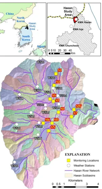
Fig. 1. Haean study area within the Lake Soyang watershed is located in northeastern South Korea along the demilitarized zone (DMZ) border with North Korea. The regional KMA weather sta-tion and local meteorological stasta-tions are denoted with white circles and (WS). River discharge monitoring locations are denoted by (S) and the yellow squares.
2 Catchment characteristics
The Haean catchment study area (38.239–38.329◦N, 128.083–128.173◦E) is located in the Gangwon Province of the northeastern portion of South Korea along the demilita-rized zone (DMZ) between South and North Korea (Fig. 1). The 62.7 km2catchment has a unique bowl-shaped physio-graphic characteristic with elevation ranging between 339 to 1321 m a.s.l., which drastically alters the local meteorologi-cal conditions. The catchment drainage is the Mandae River with a maximum length of 8.6 km. Limited historical obser-vations are available, although this is typical for most areas
outside of Europe and North America. The average catch-ment discharge at the outlet is 4.32 m3s−1(1.20–379 m3s−1) while the average discharge at the S1 headwater monitoring location is 0.03 m3s−1(1.4×10⁻⁴–10.0 m3s−1). The catch-ment hydrology is further described in Shope et al. (2013). The catchment is 56 % forested and 44 % agricultural LULC. Geologically, the basin is composed of a Precambrian gneiss complex at the higher elevation mountain ridges and a highly weathered Jurassic biotite granite intrusion that was subsequently eroded throughout the central portion of the catchment (Kwon et al., 1990). Alluvium generally extends up to 2 m in depth and bedrock is typically observed between 20 and 45 m below land surface in the catchment interior. Surficial soil texture is typically saprolitic sand and sandy loam with high infiltration capacity (Arnhold et al., 2013; Jo and Park, 2010).
The climate in South Korea is humid continental to hu-mid subtropical, influenced by the East Asian summer mon-soon and early autumn typhoons. The monmon-soon season ex-tends from the end of June through the end of July, fol-lowed by scattered events through early September, with up to 70 % of the total annual precipitation between the months of June and August. The average annual rainfall over the most recent 12 yr of record is 1514 mm (930 to 2299 mm yr−1) with a maximum precipitation as high as 48.6 mm h−1 or up to 223.2 mm d−1. The average annual temperature is 8.65±0.35◦C ranging between−26.9◦C in January to 33.4◦C in August. Choi et al. (2010) found that the temperature lapse rate within the Haean catchment ranged between−0.56◦C 100 m−1throughout the spring to +1◦C 100 m−1during early morning inversions after many consecutive sunny days.
3 Methods and model construction
3.1 Model description
subbasin and through the channel network to the watershed outlet (Neitsch et al., 2011). Incoming precipitation is par-titioned into canopy storage, infiltration, and surface runoff through either the SCS (Soil Conservation Service) curve number (CN) method (U.S.D.A., 1972) or the Green–Ampt (Green and Ampt, 1912) method. Daily runoff volume from the SCS retention parameter can be calculated through the shallow soil water content or through accumulated plant ET. The SCS curve number method with calculated plant evap-otranspiration was selected for the Haean catchment simu-lations. The hydrologic condition of the vegetation is im-portant in determining CN for individual HRUs (U.S.D.A., 1972). Therefore, the distributed CN was further modified within individual HRUs through time-variable LULC char-acterization and crop growth. The model uses the modified Rational Method to estimate peak flow (Neitsch et al., 2011). Runoff in SWAT is aggregated from the HRU level into the subbasin level and then routed through the stream network. The Manning equation is used to estimate the flow rate and velocity through the channels. Flow routing is based on either the variable storage or the Muskingum routing method; and for this study, we chose the variable storage method (Neitsch et al., 2011).
3.2 Model inputs
3.2.1 Climate data
Hourly climate data for the period from 1998 to 2011 were measured and collected from several regional stations of the Korean Meteorological Agency (KMA) (Fig. 1). Precip-itation and minimum/maximum temperature were obtained from the Haean KMA station (38.287◦N, 128.148◦E). Rel-ative humidity, temperature, and wind speed were obtained from the Inje KMA station in the adjacent Yanggu County (38.207◦N, 128.017◦E). Solar radiation was collected from the Chuncheon KMA station (37.904◦N, 127.749◦E). Dis-tributed climate data were also collected from 15 micro-meteorological stations (Delta-T Devices, Ltd.) throughout the catchment (Fig. 1) between 2009 and 2011. Sub-hourly data was aggregated into hourly precipitation (±0.2 mm), minimum/maximum air temperature (±0.2◦C), wind speed (±0.1 m s−1), solar radiation (±5 W m−2), and relative hu-midity (±2 %). Each parameter was quality controlled by re-moving erroneous data and then gap filling from a similar station using a weighted algorithm based on elevation, sta-tion proximity, and aspect. The algorithm, as formulated for precipitation, is presented as
Pe(z, d, ϕ)=
a
i=1 Pominimizevi=1(ϕe−ϕo)w3+... h
a i=1
h
dx
dx+dy
·Px−Py i
+Px
w2 i
+...
a
i=1 Pominimizevi=1(ze−zo)w1 . (1)
The variablePeis the estimated precipitation (mm),zis the elevation (m),d is the distance to the observation point (m),
φ is the observation point aspect (deg.),i is the time step,
a is the total number of consecutive missing data,Pois the observed precipitation (mm),vis the total number of obser-vational meteorological stations,j is the cumulative number of stations, the “e” and “o” subscripts are the estimated and observed location values,w is the weighting factor, and x
andysubscripts are the first and second most proximal loca-tions to the estimation location, respectively. Locally based relative humidity was modified by accounting for the tem-perature dependent local dew point. The SWAT model does not explicitly interpolate spatial meteorological conditions but instead, prescribes the nearest weather station parameters to the centroid of each subbasin (Neitsch et al., 2011). Due to the large variation in topographical complexity throughout the catchment, precipitation volume, soil moisture, and plant growth were impacted when SWAT assigned the meteoro-logical data to each subbasin. We tested several interpolation methods to grid the measured meteorology results through-out the catchment (inverse distance weighted (IDW), spline, nearest neighbor, and kriging). The IDW method performed optimally and was used to grid the measured meteorological results throughout the catchment and the virtual weather cor-responding to each subbasin centroid was prescribed. Prin-ciple data sources used for the Haean catchment ecohydro-logic model are provided in Table 1. Choi et al. (2010) found highly variable temperature lapse rates, implying that stag-nant East Asian monsoon high pressure systems can signifi-cantly vary climatic conditions on a local scale. A tempera-ture lapse rate of−0.52◦C 100 m−1 was incorporated into the continuous spatial interpolation for temperature.
3.2.2 Discharge and evapotranspiration estimates
Event-based and baseflow surface water discharge measure-ments were collected at up to 14 locations throughout the catchment between 2003 and 2011 (Fig. 1) through multi-ple methods as described by Shope et al. (2013). Observed streamflow at interior locations within the catchment (S1, S4, S5, and S6) and the catchment outlet (S7) were utilized for daily and monthly model calibration to better parameterize spatial variability in hydrologic partitioning. These monitor-ing locations are distributed throughout the catchment along an elevation gradient with increasing drainage area and pro-vide regional representation of model parameterization. In addition, the unique punchbowl shape enabled the calibration parameters to be correlated to other ungauged subcatchments with similar slope, elevation, and aspect.
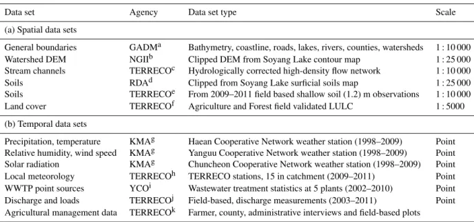
Table 1.Principle input data sets for the construction of the Haean catchment SWAT model.
Data set Agency Data set type Scale
(a) Spatial data sets
General boundaries GADMa Bathymetry, coastline, roads, lakes, rivers, counties, watersheds 1 : 10 000
Watershed DEM NGIIb Clipped DEM from Soyang Lake contour map 1 : 25 000
Stream channels TERRECOc Hydrologically corrected high-density flow network 1 : 10 000
Soils RDAd Clipped from Soyang Lake surficial soils map 1 : 25 000
Soils TERRECOe From 2009–2011 field based shallow soil (1.2) m observations 1 : 10 000
Land cover TERRECOf Agriculture and Forest field validated LULC 1 : 5000
(b) Temporal data sets
Precipitation, temperature KMAg Haean Cooperative Network weather station (1998–2009) Point
Relative humidity, wind speed KMAg Yanguu Cooperative Network weather station (1998–2009) Point
Solar radiation KMAg Chuncheon Cooperative Network weather station (1998–2009) Point
Local meteorology TERRECOh TERRECO stations, 15 in catchment (2009–2011) Point
WWTP point sources YCOi Wastewater treatment statistics at 5 plants (2002–2010) Point
Discharge and loads TERRECOj Field-based, discharge measurements (2003–2011) Point
Agricultural management data TERRECOk Farmer, county, administrative interviews and field-based plots
aGADM – Global Administrative Areas.bNGII – National Geographic Information Institute.cTERRECO – Field-based TERRECO IRTG observations, GPS
surveyed perennial and ephemeral stream channels.dRDA – Rural Development Administration.eTERRECO – Field-based TERRECO IRTG observations, 2009–2011 test pits, soil samples, soil characterization.fTERRECO – Field-based TERRECO IRTG observations, 2009 (36 classes), 2010 (114 classes), 2011 (100
classes).gKMA – Korean Meteorological Weather Station Network.hTERRECO – Field-based TERRECO IRTG observations, 2009–2011 (precipitation, temperature, relative humidity, wind speed, solar radiation.iYCO – Yanguu County Office, wastewater treatment statistics 2003–2010.jTERRECO – Field-based,
spatially distributed, discharge measurements as described in Shope et al. (2013).kTERRECO – Field-based, spatially distributed plots of example management and interviews with multiple stakeholders.
The calculated baseflow was subsequently compared to the SWAT modeled baseflow contribution.
The SWAT model also includes several methods to cal-culate potential evapotranspiration (PET) (Hargreaves and Samani, 1985; Monteith, 1965; Penman, 1948; Priestley and Taylor, 1972) depending on the observational meteo-rological data available. Because of the robust and high-frequency spatially variable micrometeorologic data avail-able through the TERRECO project, we simulated daily PET using the Penman–Monteith method (Penman, 1948). As de-scribed in Ruidisch et al. (2013) and Shope et al. (2013), the weather conditions throughout the catchment are heteroge-neous and therefore, the physically based Penman–Monteith estimates were preferred over the alternative methods. Soil evaporation and crop transpiration were estimated using the FAO Penman–Monteith equation as described in Allen et al. (1988).
3.3 Spatial data
3.3.1 DEM
The Soyang watershed 30 m resolution digital elevation model (DEM) obtained from the National Geographic In-formation Institute (NGII) was clipped to the extent of the Haean catchment boundaries (Fig. 1). The Haean catch-ment was divided into three slope classes representing steep forested high elevation (10◦to 90◦), moderately sloped
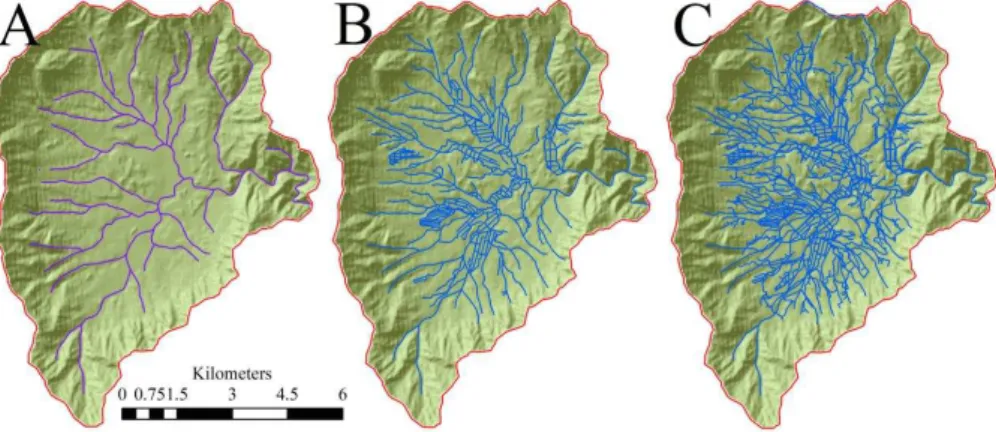
dry-land agriculture (2◦to 10◦), and mildly sloping rice paddies in the central portion of the catchment (0◦ to 2◦) (Table 2). The observed river network was geo-referenced and ex-plicitly incorporated into the DEM because modification of stream channels in highly managed catchments is prevalent and inclusion of stream delineation improves hydrologic seg-mentation and boundary delineation. In addition, extensive ground-based surveys of engineered channels, diversions, culverts, drainage features, sediment retention ponds, and roads throughout the Haean catchment were completed. To investigate the role that engineered structures have in chan-nel routing, three chanchan-nel classifications were constructed for (1) the river network; (2) the river network and engineered culverts; and (3) the river network, culvert system, and exist-ing roads (Fig. 2). We implemented the engineered structures in SWAT by sequentially adding them to the prescribed river network and we superimpose the modified networks onto the DEM. The roads and culverts were then prescribed as imper-vious channels with no transmission loss on the river net-work. Therefore, we had three complete model constructs from the beginning to the end with different hydrographic segmentation and subbasin boundary delineation.
3.3.2 Soils
–
Fig. 2.Multiple river system and infrastructure model configurations within the Haean catchment which, contribute to surface discharge accumulation and flow routing. The panels display the configuration for(A)solely the Haean river network; (B)the river network and engineered culvert drainage system; and(C)the river network, the culvert system, and the road infrastructure.
Table 2.Percentage of Haean catchment associated with the indi-vidual aggregated land use, soil, and slope classifications. The slope classification generally defines the difference between forest, dry-land farming, and rice paddy systems throughout Haean.
Area Percent
Category (km2) watershed
Landuse
Barren soil 5.92 9.43 %
General beans 1.63 2.60 %
Rice 8.53 13.59 %
General cabbage 3.21 5.12 %
Coniferous forest 0.04 0.06 %
Deciduous forest 35.29 56.25 %
Ginseng 0.81 1.29 %
Inland water 0.03 0.04 %
Residential land use 1.05 1.67 %
Maize 0.52 0.83 %
General orchards 0.86 1.36 %
Potato 2.47 3.93 %
Radish 2.12 3.38 %
Codonopsis 0.28 0.44 %
Soils
Flat dry soil 8.07 12.87 %
Forest soil 19.74 31.46 %
Moderately steep dry soil 8.33 13.28 %
Rice paddy soil 13.78 21.96 %
Sealed ground 12.47 19.87 %
Very steep forest soil 0.35 0.55 %
Slope
Low slope rice paddy 8.02 12.79 %
Moderate slope dryland 17.43 27.78 %
Steep slope forest uplands 37.28 59.43 %
(TERRECO) coupled the RDA soil data, LULC, and exten-sive field-based soil profiles to develop a spatial distribu-tion of multiple soil horizons to a depth of 3 m. Our results found that Haean soils are intensively managed and modified and highly dependent on land use (Tenhunen et al., 2011). Soil properties, including the hydrologic soil group, texture class, the percentage content of rock, sand, silt, and clay content, and the hydraulic conductivity, were derived from a 2009 catchment-wide field survey that was aggregated into 6 unique soil types (Table 2). The hydrologic group and tex-ture for each of the soils is (1) very steep forest soil (C, loam-sand), (2) forest soil (C, loam-loam-sand), (3) moderately steep dry soil (D, sand-silt), (4) flat dryland soil (D, sand-silt), (5) rice paddy soil (C, sand), and (6) sealed ground (D, clay).
3.3.3 Land use and land cover (LULC)
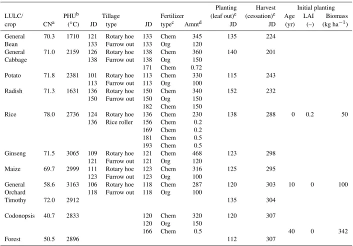
Table 3.Agricultural crop management schedule including planting and harvest dates, fertilization dates, amounts, and type of fertilizer, tilling dates and method, SCS curve number for each crop, and the heat units required to reach maturity.
Planting Harvest Initial planting LULC/ PHUb Tillage Fertilizer (leaf out)e (cessation)e Age LAI Biomass
crop CNa (◦C) JD type JD typec Amntd JD JD (yr) (–) (kg ha−1)
General 70.3 1710 121 Rotary hoe 133 Chem 345 135 224
Bean 133 Furrow out 133 Org 120
General 71.0 2159 126 Rotary hoe 138 Chem 360 140 201
Cabbage 138 Furrow out 138 Org 150
171 Chem 0.72
Potato 71.8 2381 101 Rotary hoe 113 Chem 330 115 243
113 Furrow out 113 Org 100
Radish 71.3 1631 136 Rotary hoe 150 Chem 340 152 232
150 Furrow out 150 Org 150
182 Chem 150
Rice 78.0 2736 124 Rotary hoe 136 Chem 230 138 288 0 0.2 50
136 Rice roller 156 Chem 0.2
169 Chem 0.2
181 Chem 0.5
193 Chem 0.5
Ginseng 71.5 3065 109 Rotary hoe 121 Chem 468 123 298
121 Furrow out 121 Org 120
Maize 69.7 2999 111 Rotary hoe 123 Chem 316 125 295
123 Furrow out 123 Org 100
General 58.6 3163 106 Rotary hoe 118 Chem 287 120 303 10 0 100
Orchard 118 Furrow out 118 Org 100
Timothy 72.0 2912 135 304
Codonopsis 40.7 2833 120 Chem 320 120 307
120 Org 150
166 Chem 0.5 40 0 342
Forest 50.5 2896 112 307
aCN is the SCS curve number.bPHU is the cumulative heat units above 0.0◦C required for the LULC/crop to reach maturity.cFertilizer type is classified as Chem
(inorganic chemical) not explicitly described or Org (organic manure).dFertilizer amount (kg ha−1).eLeaf out and cessation define the beginning and end of season
for forest and orchard land use.
3.4 Management inputs and crop parameterization
3.4.1 Management parameter estimation
Agricultural management practices within the Haean catch-ment were surveyed between 2009 through 2011 through a combination of on-site stakeholder interviews, empirical field observations (Tenhunen et al., 2011), published litera-ture (i.e., Nguyen et al., 2012), and regulatory reports from the Research Institute of Gangwon (RIG), the Ministry of Environment, the National Institute of Agricultural Science, and Technology and the Korean Forest Research Institute. More than 300 interviews of stakeholders and farmers were completed under the TERRECO project to quantify fertiliza-tion and pesticide applicafertiliza-tion quantities and timing, irriga-tion practices, planting and harvesting activities, and tillage methodologies. TERRECO managed plots were also used to obtain comprehensive temperature-based planting, fertil-izer, tillage, mulching, development, and harvest information (J. Tenhunen, unpublished data). An example of the land use and crop management schedule, application rate, and
appli-cation frequency is provided in Table 3. Fertilizer appliappli-cation parameters within the SWAT database were varied for each crop and subbasin for spatially distributed management. The simulated timing of management actions (i.e., fertilization, tillage, planting, irrigation, harvesting) was implemented in SWAT through daily heat unit summations because tradi-tional planting and harvest methods are dependent on cli-matic observations closely correlated to heat units.
3.4.2 Biomass sampling, analysis, and plant growth
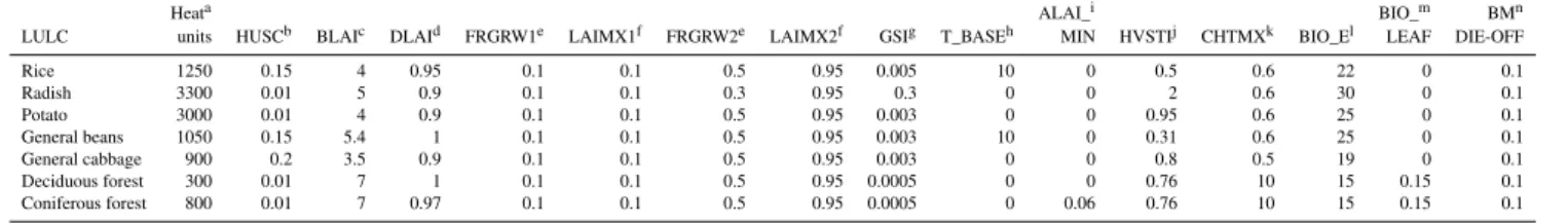
Table 4.Example SWAT model crop parameter database variations in the Haean model.
Heata ALAI_i BIO_m BMn
LULC units HUSCb BLAIc DLAId FRGRW1e LAIMX1f FRGRW2e LAIMX2f GSIg T_BASEh MIN HVSTIj CHTMXk BIO_El LEAF DIE-OFF
Rice 1250 0.15 4 0.95 0.1 0.1 0.5 0.95 0.005 10 0 0.5 0.6 22 0 0.1 Radish 3300 0.01 5 0.9 0.1 0.1 0.3 0.95 0.3 0 0 2 0.6 30 0 0.1 Potato 3000 0.01 4 0.9 0.1 0.1 0.5 0.95 0.003 0 0 0.95 0.6 25 0 0.1 General beans 1050 0.15 5.4 1 0.1 0.1 0.5 0.95 0.003 10 0 0.31 0.6 25 0 0.1 General cabbage 900 0.2 3.5 0.9 0.1 0.1 0.5 0.95 0.003 0 0 0.8 0.5 19 0 0.1 Deciduous forest 300 0.01 7 1 0.1 0.1 0.5 0.95 0.0005 0 0 0.76 10 15 0.15 0.1 Coniferous forest 800 0.01 7 0.97 0.1 0.1 0.5 0.95 0.0005 0 0.06 0.76 10 15 0.15 0.1 aHeat Units is the total base zero annual heat units for the plant cover/land use to reach maturity.bHUSC is the fraction of the total base zero annual heat units at which the
management operation occurs.cBLAI is the maximum potential leaf area index.dDLAI is the fraction of the growing season when the leaf area begins to decline.eFRGRW1,2 represent the fraction of the plant growing season corresponding to the 1st and 2nd point on the optimal leaf area development curve.fLAIMX 1,2 represent the fraction of the
maximum leaf area index corresponding to the 1st and 2nd point on the optimal leaf area development curve.gGSI is the maxixmum stomatal conductance at high solar radiation
and low vapor pressure deficit (m s−1).hT_BASE is the minimum or base temperature for plant growth (◦C).iALAI_MIN is the minimum leaf area index for the plant during
the dormant period (m2m−2).jHVSTI is the fraction of aboveground biomass removed during a harvest operation and lost from the system.kCHTMX is the maximum canopy
height (m).lBIO_E is the radiation use efficiency or biomass energy ratio ((kg ha−1)/(MJ m−2)).mBIO_LEAF is the fraction of tree biomass accumulated each year that is
converted to residue during dormancy.nBMDIEOFF is the biomass die-off fraction.
To differentiate between crop types particular to South Ko-rea (i.e., ginseng), several modified land use classes were cre-ated in the SWAT crop database. Nine representative field plots along an elevation transect were analyzed and crop pa-rameters were varied to minimize the simulated and observed residuals for leaf area index (LAI), biomass, and crop yield. The crop parameters were altered based on observed mea-surements, plant physiology modeling results from the PIX-GRO model (i.e., Adiku et al., 2006), and published litera-ture. The crop parameters that were varied are presented in Tables 3 and 4. Intensive cultivation was also present in agri-cultural areas not serviced by irrigation canals and therefore, groundwater abstraction was estimated from the PIXGRO model as the quantity required for optimal plant growth. Typ-ical to many Asian catchments, Haean can be considered a highly managed catchment with increased uncertainty due to insufficient spatiotemporal water management data.
3.4.3 Rice paddies, potholes, and water abstraction
The quantity and timing of river and groundwater abstrac-tions is uncontrolled and local estimates were inadequate for model inclusion. Depending on the HRU location, ir-rigation water was extracted from an adjacent river reach or from shallow groundwater. Groundwater-derived irriga-tion practices were limited to orchards and rice paddies and were accounted for in the simulations through water avail-ability based auto-irrigation at the HRU level and defined by the soil water deficit. Haean rice paddies were simu-lated in SWAT as potholes, which are hydrologically simi-lar to ponded areas. Rice paddies are typically characterized by multiple cascading-elevation plots separated by embank-ments. The rice paddies had low infiltration and typically sat-urated soil conditions and therefore, infiltration as a function of water content rather than flow routing was used for esti-mation of subsurface losses. The HRUs within each subbasin were developed using 0 % land use and 0 % slope threshold for reach subbasins resulting in maximum number of HRUs. Since a subbasin can have multiple HRUs but only have a
single pothole, we limited the rice paddies in each subbasin to a single HRU. We accomplished this by varying the soil threshold until only a single rice paddy HRU was in each of the subbasins.
4 Results and discussion
4.1 Meteorological drivers and the effects of interpolation
Meteorological time series data, particularly precipitation is a highly sensitive driver in hydrologic modeling applications (Strauch et al., 2012). Spatial monitoring distributions are typically limited and do not capture heterogeneous meteoro-logical conditions that can be interpolated by wide-meshed monitoring networks (Notter et al., 2007). Large variations in elevation throughout the Haean catchment influence the precipitation volume, soil moisture, and plant growth. They can also influence the peak flow and the time of concentra-tion to peak discharge of the simulated hydrograph (Khak-baz et al., 2012; Wilson et al., 1979). Our weather analysis revealed heterogeneous meteorological conditions through-out the Haean catchment that are dependent on elevation and aspect and largely focused in subregions (Choi et al., 2010; Shope et al., 2013). These meteorological variations have a direct influence on the relative humidity and therefore, the spatial variability of plant growth parameters between sub-basins was significant (Fig. 3).
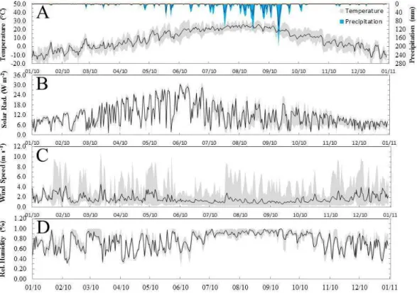
Figure 3 – Meteorologic variability and average daily value of each variable throughout the
Fig. 3.Meteorologic variability and average daily value of each variable throughout the Haean catchment for 2010.(A)describes the daily precipitation and temperature variability,(B)is the range in solar radiation and the average value between all of the locations,(C)is the wind speed variability, and(D)is the relative humidity range.
improved plant growth response for selected crops and lo-cations than other methods. Similar to results obtained by Notter et al. (2012), the IDW method was invoked to develop a continuous grid of meteorological drivers that were subse-quently assigned to individual subbasins.
4.2 Model calibration, validation, and uncertainty assessment
4.2.1 Sensitivity and model parameterization
The model sensitivity was addressed with respect to spa-tial distribution (number and location of meteorological sta-tions, LULC distribution), observational record (LULC cov-erages, meteorological stations), resolution (soil coverage, subbasin discretization), and hydrologic stimulus (rainfall– runoff). The Haean catchment model configuration resulted in 142 topographically based subbasins and 2532 individual HRUs. Previous investigations have shown that the number of subbasins has little influence on runoff (Jha et al., 2004; Tripathi et al., 2006; Xu et al., 2012a, b). Alternatively, other studies have found that HRU discretization can have a sub-stantial effect depending on the physical catchment condi-tions, data quality, and investigative scale (i.e., Setegn et al., 2008; Haverkamp et al., 2002). We assessed the effect of subbasin size and HRU definition on surface water
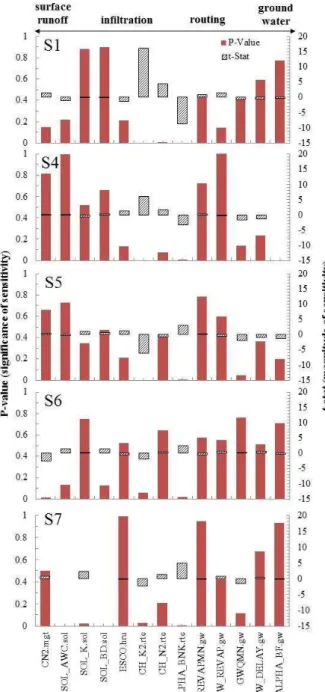
dis-charge and found no appreciable difference between model results. However, our results show that elevation-based plant parameters and convective precipitation captured through in-creased subbasin discretization can be important. Subbasins with steep slopes and extensive vertical gradients must ac-count for elevation-based climate conditions, which con-tribute to highly variable ET conditions. The sensitivity anal-ysis of discharge related model parameters was achieved by sequentially varying an individual parameter while maintain-ing the remainmaintain-ing parameters for each monitormaintain-ing location. Between eight and eleven parameters from the original 15 discharge-related parameters were found to be sensitive to catchment-wide flow partitioning (Fig. 4). Subsequently, the range of each of the parameters was minimized during cali-bration procedures.
Fig. 4.SWAT simulated parameter sensitivity (pvalue) and model significance (ttest) for the Haean catchment for monitoring loca-tions S1, S4, S5, S6, and S7 along the elevation transect.
Therefore, for computational efficiency, a semi-distributed approach was taken throughout the catchment utilizing the most sensitive parameters at each monitoring location for pa-rameterization in adjacent areas.
While we did not explicitly quantify the optimal param-eterization, through a series of iterations we weighted the objective functions (R2, NSE, PBIAS, and baseflow percent-age) in decreasing order as we compared individual locations throughout the catchment. In effect, we used a multi-criteria
decision making process to determine the relative priority of each alternative when all of the criteria were considered si-multaneously. Because our results indicated that the sensi-tivity analysis was significantly based on the monitoring lo-cation, we calibrated multiple locations along an elevation transect. In Fig. 4, the “tstat” provides a measure of parame-ter sensitivity where larger absolute values are more sensitive and the “pvalue” determines the significance of sensitivity with higher significance as values approach zero (Abbaspour, 2011).
Our results generally indicate surface runoff and routing parameters are more sensitive at higher elevations with in-creasing sensitivity to infiltration and groundwater param-eters at lower elevations (Fig. 4). The REVAPMN ground-water parameter was a sensitive parameter at each location; however, the magnitude was relatively small. CH_K(2) was the least sensitive parameter, although included in the analy-sis for comparison. Table 6 provides a summary of the SWAT parameters. The infiltration parameters suggest significant baseflow response at higher elevations. At mid-elevations, surface runoff and routing parameters become more sen-sitive. At lower catchment elevations, infiltration, routing, and groundwater parameters dominate. Since the upper el-evation locations are composed of shallow, highly perme-able (S. Arnhold, unpublished results) soils over bedrock; we conceptualize high infiltration rates that contribute to in-creased baseflow and streamflow accumulation. At mid- to low-elevation locations, higher land management and soil amendments lead to runoff and less infiltration. These results identify the importance of and differences between model sensitivities as a function of the model equations, model sensitivity, and observational dynamics. Therefore, caution should be exercised in rainfall–runoff process simulations in relatively ungauged basins.
4.2.2 Metrics of model performance for calibration
procedures
Model performance was assessed by several metrics at each location including the simulated and observed water balance, the coefficient of determination (R2), Nash–Sutcliffe effi-ciency (NSE), percentage bias (PBIAS), and the baseflow contribution. The R2 was used to evaluate time and space
L.
Shope
et
al.:
Landscape
complexity
and
ecosystem
modeling
with
the
SW
A
T
mo
del
549
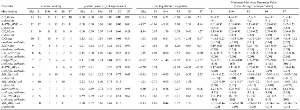
Table 5.SWAT parameter sensitivity and significance between discharge parameters throughout the Haean catchment (Fig. 4). Calibrated SWAT parameters for the Haean catchment, including the individual ranking along the elevation-based transect, the minimum and maximum parameter values for all subbasins accounted for by each monitoring location, and the average calibrated parameter value. Because of the distributed nature of the Haean model, individual parameters varied depending on crop type, elevation, aspect and therefore, a specific parameter value is not available.
Minimum–Maximum Parameter Value Parameter Parameter ranking pvalue (sensitivity of significance) tstat (significance magnitude) [Final Average Parameter Value]
(distribution) S1a S1 S4W S5 S6 S7 S1a S1 S4w S5 S6 S7 S1a S1 S4w S5 S6 S7 S1 S4W S5 S6 S7
CH_K2.rte 13 13 12 13 12 10 0.00 0.00 0.00 0.00 0.06 0.03 16.23 6.01 6.21 −6.18 −1.89 −2.21 81–139 43–139 −51–70 24–117 51–143
(subbasin) [94] [83] [9.2] [71] [97]
ALPHA_BNK.rte 12 12 8 12 13 11 0.00 0.00 0.00 0.00 0.02 0.00 −8.77 −3.68 −3.18 3.10 2.34 4.94 0.01–0.35 0.05–0.80 0.15–0.87 0.28–0.92 0.42–1.25
(subbasin) [0.34] [0.22] [0.51] [0.60] [0.83]
CH_N2.rte 11 9 11 11 9 9 0.00 0.39 0.07 0.43 0.64 0.21 4.44 0.87 1.79 -0.79 0.46 1.27 0.13–0.39 0.08–0.31 0.03–0.22 0.08–0.30 0.06–0.29
(subbasin) [0.26] [0.17] [0.12] [0.19] [0.17]
CN2.mgt 10 11 10 9 5 4 0.15 0.11 0.81 0.66 0.01 0.50 1.43 1.62 0.24 0.44 −2.51 0.67 −0.62–0.23 −0.55–0.36 −0.32–0.54 −0.33–0.60 −0.38–0.52
(land use, subbasin) [−0.58] [−0.05] [0.11] [0.14] [0.07]
ESCO.hru 9 7 6 5 3 2 0.21 0.42 0.13 0.21 0.52 0.99 −1.24 0.81 1.51 1.26 −0.64 −0.01 0.19–0.89 0.16–0.91 0.25–1.01 0.13–0.89 0.21–0.97
(land use, subbasin) [0.39] [0.55] [0.63] [0.51] [0.59]
GW_REVAP.gw 8 6 1 1 2 5 0.15 0.30 1.00 0.60 0.55 0.42 1.45 1.05 0.00 −0.53 0.60 0.80 0.06–0.16 0.05–0.18 0.03–0.15 0.02–0.16 0.03–0.16
(soil type, subbasin) [0.09] [0.09] [0.09] [0.09] [0.10]
GWQMN.gw 7 2 5 4 4 7 0.41 0.60 0.14 0.04 0.76 0.12 −0.82 0.52 −1.48 −2.02 0.30 −1.57 32–4151 1370–4800 512–3596 323–3894 1133–4890
(soil type, subbasin) [475] [2675] [2054] [2108] [3011]
ALPHA_BF.gw 6 1 6 6 8 0.77 0.81 0.20 0.71 0.93 −0.29 0.24 −1.29 −0.37 −0.08 0.12–0.46 0.11–0.52 0.02–0.39 0.00–0.38 0.08–0.46
(soil type, subbasin) [0.20] [0.22] [0.21] [0.19] [0.27]
SOL_K(1).sol 5 3 9 10 1 6 0.88 0.61 0.52 0.35 0.75 0.03 −0.15 0.51 −0.65 0.94 0.32 2.25 −1.46–0.22 −0.56–0.71 −0.64–0.85 −0.90–0.42 −0.85–0.56
(subbasin) [−0.78] [0.10] [0.10] [−0.24] [−0.15]
SOL_AWC(1).sol 4 10 4 3 10 0.22 0.43 1.00 0.73 0.13 −1.23 −0.79 0.00 −0.35 1.51 −0.20–0.39 −0.41–0.47 −0.56–0.21 −0.49–0.48 −0.67–0.18
(subbasin) [0.30] [0.02] [−0.17] [−0.01] [−0.25]
REVAPMN.gw 3 4 7 7 7 1 0.43 0.69 0.72 0.79 0.58 0.95 0.80 −0.41 0.36 0.27 −0.56 −0.06 2.73–6.74 1.98–9.53 0.41–8.62 1.42–8.36 1.62–9.13
(soil type, subbasin) [4.72] [6.14] [4.51] [4.89] [5.38]
GW_DELAY.gw 2 5 3 8 8 3 0.59 0.39 0.23 0.36 0.51 0.67 −0.53 0.88 −1.19 −0.91 0.66 0.42 138–453 16–334 73–412 −28–322 31–362
(soil type, subbasin) [398] [202] [242] [147] [197]
SOL_BD(1).sol 1 8 2 2 11 0.90 0.07 0.66 0.47 0.13 −0.13 1.85 0.44 0.72 1.53 −0.36–0.44 −0.43–0.30 −0.62–0.13 −0.34–0.36 −0.34–0.35
(subbasin) [−0.25] [−0.05] [−0.25] [0.01] [0.01]
.h
ydr
ol-earth-syst-sci.ne
t/18/539/2014/
Hydr
ol.
Earth
Syst.
Sci.,
18,
539–
557,
sources. This metric provides an independent check on a spe-cific component of the water budget. Finally, measured plant growth dynamics were compared with simulated results.
4.2.3 Manual and automated model calibration
Due to the complexity of large-scale multi-objective anal-yses, watershed models are typically highly parameterized and manual calibration can be virtually impossible (Schuol and Abbaspour, 2006) although multi-site, multi-objective inverse calibration and uncertainty analysis can aid in un-derstanding the system (Abbaspour et al., 2004; Duan et al., 2003). Model calibration was separated into two com-ponents, (1) manual catchment-scale calibration to estimate system processes and variability, and (2) automated calibra-tion to quantify model uncertainty.
The SWAT model was simulated from 2006 through 2011 with the first 3 yr excluded for model initialization. The cali-bration and validation of river discharge was performed at a daily time step from 2009 through 2011, with 2010 as the cal-ibration period and 2009 as the validation period. For loca-tions S4 and S6, we did not have observational records for the 2009 validation period and instead used the concept of self-similarity for validation results. Since the transect followed an elevation gradient in a limited portion of the catchment, we conceptualized that similar hydrologic processes were oc-curring for similar elevation and drainage areas in other parts of the catchment. For example, location S4 was calibrated to the 2010 observational data, although there was limited data to validate for 2009. Because SD and SK had similar topography, elevation, drainage area, and land use pattern-ing as S4 and S6, respectively, they were used to validate the S4 calibration parameters. Intensive manual calibration was performed at each of the subbasins routed to a monitoring station and used to minimize the acceptable parameter range at each site. The difficulty is that manual calibration sensitiv-ity suffers from the linearsensitiv-ity assumption by not accounting for correlations between individual parameters.
After manual calibration was optimized through the weighted, multi-criteria metrics previously discussed, auto-mated model calibration, validation, and uncertainty anal-ysis was completed using the Sequential Uncertainty Fit-ting Algorithm (SUFI-2) (Abbaspour et al., 2004, 2007). The manual calibration results provided distributed, physi-cally based parameter ranges that were incorporated into the SUFI-2 auto-calibration routine, starting with the catchment outlet and following a top to bottom approach. Model uncer-tainty in auto-calibration is quantified by the 95 % prediction uncertainty (95PPU) at the 2.5 and 97.5 % cumulative dis-tribution, which is obtained through Latin hypercube sam-pling procedure (Abbaspour et al., 2004). Because the model varies multiple parameters at the same time, two indices are used to assess the stochastic calibration performance. The “pfactor” describes the percentage of data bracketed by the 95 % prediction uncertainty and the “rfactor” describes the
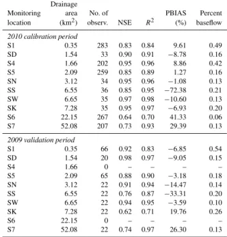
Table 6.Calibration and validation statistics for each of the moni-toring locations throughout the Haean Catchment. The data includes the subbasin demarcation of the monitoring locations, the total num-ber of observations, the observed and simulated water balance, the NSE, R2, and PBIAS statistics, and the percent baseflow contribu-tion.
Drainage
Monitoring area No. of PBIAS Percent
location (km2) observ. NSE R2 (%) baseflow
2010 calibration period
S1 0.35 283 0.83 0.84 9.61 0.49
SD 1.54 33 0.90 0.91 −8.78 0.16
S4 1.66 202 0.95 0.96 8.86 0.42
S5 2.09 259 0.85 0.89 1.27 0.16
SN 3.12 34 0.95 0.96 −1.08 0.13
SS 6.55 36 0.85 0.95 −72.38 0.21
SW 6.65 35 0.97 0.98 −10.60 0.13
SK 7.28 35 0.95 0.97 −6.93 0.20
S6 22.15 267 0.64 0.70 41.33 0.06
S7 52.08 207 0.73 0.93 29.39 0.13
2009 validation period
S1 0.35 66 0.92 0.83 −6.85 0.54
SD 1.54 20 0.98 0.97 −9.05 0.15
S4 1.66 0 – – – –
S5 2.09 65 0.88 0.90 −3.18 0.18
SN 3.12 22 0.91 0.94 −14.47 0.14
SS 6.55 22 0.76 0.87 −33.31 0.20
SW 6.65 22 0.94 0.95 −3.59 0.10
SK 7.28 22 0.62 0.71 19.76 0.26
S6 22.15 0 – – – –
S7 52.08 22 0.74 0.97 26.30 0.13
average width of the prediction band divided by the stan-dard deviation of the measured data (Faramarzi et al., 2009). Since the uncertainty in field-based river discharge measure-ments was typically <5 % (Shope et al., 2013), a conser-vative 10 % measurement error was included in the “p and
r factor” calculations (Abbaspour et al., 2009; Andersson et al., 2009; Butts et al., 2004; Schuol et al., 2008). Yang et al. (2008) found that reasonable prediction uncertainty ranges were achieved with 1500 model simulation iterations, while, (Güngör and Göncü, 2012) showed that 300 iterations provided similar results to 1500 iterations. In Haean, at least 300 simulation iterations at each location were performed throughout the auto-calibration routine (Table 5).
As described, the calibration parameters were selected to optimize the PBIAS,R2, and NSE test statistics, the
were calibrated to account for daily trends by maximizing the NSE. When the Muskingum routing method was utilized, the channel parameters CH_N(2) and CH_K(2) were ranked 2 and 3 in the sensitivity analysis. However, the relative change in NSE between outlet results was negligible (∼0.01) com-pared to the default variable storage routing method, and the addition of more parameters was substantial. Therefore, vari-able storage routing within the SWAT model was chosen to limit the model parameterization.
The explanation for the deviations in runoff at the low elevation locations (S6 and S7) is not known or reflected in the SWAT input data. However, by examining a combi-nation of optimized calibrated data, process-based compar-isons, and field observations, the overall calibration metrics indicated increased flow routing directly from high elevation locations to lower elevation river locations. A possible ex-planation is the density of surface water collection and sedi-mentation ponds within the catchment, which may have im-pacted the observed runoff characteristics of the watershed (Cho et al., 2012). Using a multi-criteria optimization ap-proach, we identified that engineered flow routing and infras-tructure construction such as roads and culverts, contributed to increased discharge at lower elevations. These catchment-wide landscape engineering results are further discussed in Sect. 4.5.
4.3 Spatiotemporal flow partitioning with respect to river discharge
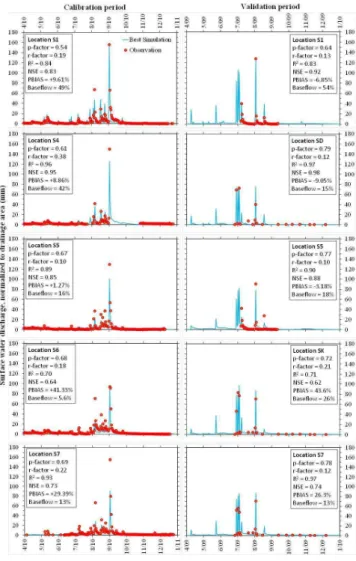
The calibration and validation of the Haean catchment daily discharge yielded good results given the scarcity and the tem-poral longevity of the available data. The modeling results indicated that SWAT performance at the Haean catchment re-lied heavily on the quality and more importantly abundance of discharge data, similar to the results of Dessu and Me-lesse (2012). The NSE score for monitoring locations S1, S4, S5, S6, and S7 ranged between 0.64 and 0.95 with an aver-age score of 0.76 for the 2010 calibration period and between 0.40 and 0.98 for the validation period (Fig. 5). Satisfactory NSE scores of>0.5 (Moriasi et al., 2007) were achieved at all 14 gauge locations in the calibration period and at 12 of 14 in the validation period. TheR2value was also reasonable
for each of the monitoring locations, ranging from 0.70 to 0.96 with an average value of 0.81 for the calibration period and between 0.71 and 0.97 for the validation period (Fig. 5). The fact that similar performance measures were reached in both validation and calibration periods indicate that there was minimal “overfitting” of the distributed parameters.
The baseflow contribution estimated at monitoring loca-tion S4 using a digital filter hydrograph separaloca-tion technique was 26 %, although the calibrated estimate was 42 %. The hy-drograph separation magnitude varied significantly, depend-ing on the data quality, the length of the analysis, and the time step investigated. However, the digital filter methodology for estimation of the hydrograph separation is not process-based
Fig. 5.Calibrated and validated daily comparison of drainage area normalized observed and simulated river discharge along the eleva-tion transect of monitoring locaeleva-tions S1, S4, S5, S6, and the catch-ment outlet S7. Included on each panel are the objective function and optimization statistics.
and may have significant uncertainty. The calibrated base-flow of 42 % at S4 is similar to the estimate at the upstream location S1 and nearly twice as high as all of the down-stream locations, indicating that this mid-elevation area may be transition zone between baseflow and runoff dominated streamflow. This suggests that high elevation locations have increased baseflow contributions, relative to low elevation lo-cations, regardless of the observational data period.
Table 7.Biomass production and crop yield statistics for South Korea and specifically, for the Haean catchment.
Average S Korea cultivation 2009 Haean 2009 LULC area 2009 Haean
Area Production Yield Plot Yield Plot Haean Crop Yield
(ha) (metric tn) (tn ha−1) (tn ha−1) (ha) (ha) (tn)
Rice 936 766 6 869 305 7.33 11.26 13.32 87 312 73 796
Cabbage 34 321 2 542 000 74.07 4.81 10.35 32 742 15 226
Potato 26 804 600 000 22.38 22.94 1.17 25,038 490 895
Radish 23 780 1 223 000 51.43 35.24 1.26 21 828 610 422
Soybean 80 505 137 000 1.70 14.66 0.09 16 692 2 719 127
Deciduous forest – – – 42.03 103.05 359 520 146 620
Sources: Ministry for Food, Agriculture, Forestry & Fisheries (MIFAFF), Korea Rural Economic Institute, Korean Statistical Information Service (KOSIS), Korea Agro-Fisheries Trade Corp. (aT), Yanggu statistical year-book 2003–2011 from the Yanggu County Office, FAOSTAT 2008, World Bank 2009.
that were routed through culverts, drainages, and road sys-tems to lower catchment locations. Essentially, the effect of the anthropogenic routing not only creates a large disparity in simulated discharge, but limits the subsurface infiltration at the plot-scale for higher elevation locations and surrep-titiously develops a misleading flashy flow system with re-duced landscape water storage.
The lower NSE score andR2 values could be attributed to the low magnitude relative variability of discharge at higher elevation monitoring locations, which contributes to increased deviations of NSE scores during event conditions, particularly monsoonal extreme events. At location SK, there is scarce observation data and because the NSE statistics weight extreme events higher, limited but high deviations have a much larger impact than minor deviations. In addi-tion, the difficulty in accurately simulating the river discharge at monitoring location SK was hypothesized to be a func-tion of high elevafunc-tion flow contribufunc-tions that bypassed the monitoring gage as hyporheic flow (Shope et al., 2013). The hydrological response throughout East Asia and within the Haean catchment in particular, is typically flashy and erratic, further attributing to event-based deviations in the objective functions. At monitoring location S5, a higher temporal den-sity of observations was obtained and the model performance metrics are generally better than for other locations.
Overall, the calibration and validation results were good and the percentage of baseflow contribution at each location was reasonable in terms of the hydrograph separation esti-mates. The auto calibration metrics of p-value andrvalue are both reasonable, while theR2and NSE statistics were consis-tently above satisfactory and predominately considered very good. The averagepfactor throughout the calibration period at all stations was 0.64 (0.54 to 0.69) and ther factor was
0.21 (0.10 to 0.38). The averagepfactor andr factor from
the validation period was 0.74 (0.64 to 0.79) and 0.14 (0.10 to 0.21), respectively (Fig. 5). This indicates that the major-ity of the simulated results were within the 95 % confidence interval and that the standard deviation was adequately mini-mized. As shown in Fig. 5 and Table 7, the validation results
–
Fig. 6.Daily heat sum estimate between 1998 and 2010 for the S1 forest boundary monitoring location within the Haean watershed (Fig. 1).
at these locations were good and consistent with the results estimated at the calibration locations.
Each of the objective functions, hydrologic partitioning quantified by PBIAS, and the baseflow percentages were cal-ibrated simultaneously, which while optimizing the values of some parameters, were at the detriment of other parameters. For example, the NSE at S5 was initially 0.89; however, pa-rameter adjustments were made to minimize the water bal-ance, which resulted in a lower NSE value. The event on 1 September 2010 had a major influence on the magnitude of the NSE andR2objective function. This is primarily due to the paucity of observation points and therefore, the weight of individual points on the overall relationship, particularly during peak events.
Fig. 7.Comparison of simulated versus observed leaf area index (LAI) for five of the primary crops grown in Haean and the deciduous forest.
estimated river discharge (Shope et al., 2013) or the short du-ration of observational data, significantly affected the model performance. For example, extensive observational data was collected at S5 but more limited at S4 and S6, resulting in decreased statistics at the latter location, even after calibra-tion. The relatively large 95 PPU band “rfactor” necessary to bracket the observed data indicates that the uncertainty in the conceptual model is also very important for the Haean catchment.
4.4 Agricultural management and production
The heat sum methodology used to estimate time variable management and planting actions, provides the flexibility to account for unseasonable variations in meteorological drivers between years (Fig. 3). Heat sums are calculated as the cu-mulative daily temperature greater than the base temperature of 0.0◦C initiated on the planting date and completed at the maximum growth. The HUSC is the percentage of the total heat units necessary for optimal growth of an individual crop and is prescribed for each management activity. The mini-mum heat sum over the period of record was 4246◦C dur-ing 2009, the maximum was 5783◦C during 2003, and the average annual heat sum is 5222◦C (Fig. 6). The 12 yr lin-ear trend line of maximum cumulative annual heat sum val-ues indicates a general decrease of nearly 74.8◦C per year. When the potentially extreme years of 2003, 2008, and 2009 were excluded, a decrease of 15.3◦C per year was estimated. While precipitation trends suggest more extreme events oc-curring over a shorter time, these results indicate a decreas-ing trend in annual heat output necessary for optimal plant growth.
To evaluate the SWAT simulation results on the ecohydro-logic response, we also analyzed the simulation results in
terms of agricultural growth dynamics at selected plot loca-tions throughout the catchment. While calibrating spatiotem-poral discharge as previously described, we also investigated the effect of crop dynamics through temporal leaf area index (LAI) as a proxy for crop growth and development (Fig. 7). Individual crop growth and development parameters were ad-justed for a comparison between observed and simulated LAI (Table 4). Results indicate a generally reasonable approxi-mation of simulated LAI where theR2for each of the crop types ranged from 0.51 to 0.76 (Fig. 7). More importantly, the results provide a consistent estimate of temporal trends in simulated biomass or agricultural production.
4.5 Influence of engineered landscape structure
(Fig. 2). As previously described in Sect. 4.3, the model per-formance in terms of PBIAS decreased toward the catchment outlet, particularly near S6 and S7. As the transect continues to the catchment outlet, the p factor decreases from 71 to 11 %, indicating that less data is bracketed by the 95 % con-fidence interval, while the r factor describing the standard deviation of the observed discharge increases from 0.20 to 0.36.
When the model was reconfigured to account for both the river drainage network and the culverts, a better calibration was obtained where the PBIAS at monitoring locations S6 and S7 decreased from 41 and 29 % to 8 and 9 %, respec-tively. The dramatic difference in PBIAS was not extended by including the roads into the river and culvert drainage network with a negligible increase in PBIAS observed at S6 and S7. Therefore, inclusion of the field-based drainage cul-verts was effective in moderating the difference in observed and model computed river discharge at lower elevation mon-itoring points and consistent with field-based observations of event-peak flow routing through the Haean watershed. How-ever, it is surprising that the road network had minimal influ-ence. During peak event conditions, substantial overland flow and sediment transport was observed throughout the Haean catchment. Since the poured concrete culverts are immedi-ately adjacent to many of the plots, reduced landscape-scale infiltration required to maintain local soil moisture storage and rapidly transported excessive nutrients from fertilizer applications into the lower parts of the catchment is preva-lent. This results in a rapid transport of elevated nutrient and sediment loads into the river. Therefore, while there is a significant influence on landscape-scale surface runoff, river discharge, and effectively hydrologic partitioning, a poten-tially greater issue is the impact expected from the rapid and large-scale alteration in water quality.
5 Conclusions
To provide a high accuracy estimate of spatiotemporal me-teorological conditions, we used a unique high-frequency, quality control, and gap-filling algorithm to develop a de-tailed interpolation of weather patterns. The interpolated me-teorological conditions were then discretized throughout the catchment and the conditions were prescribed at the centroid of each of the subbasins. This novel technique provided a better estimate of the dynamic variability due to convective storm events than the default SWAT application of prescrib-ing the nearest weather station to the subbasin centroid.
We demonstrate that the use of a novel catchment-wide, multi-location, multi-objective function approach can dras-tically improve process-based estimates of catchment-wide hydrologic partitioning. By calibrating the model to many lo-cations distributed throughout the catchment, landscape con-trols on hydrologic partitioning can be estimated as opposed to the integrated effect simulated at the catchment outlet.
Be-cause the catchment is essentially a bowl-shaped topographic feature, the concept of symmetry enabled the results from a single elevation-based transect of monitoring locations to be utilized in a catchment-wide model calibration and vali-dation. Our results showed that a combination of statistical, hydrologic, and plant growth objective functions as model-ing metrics provide a more comprehensive understandmodel-ing of system interactions. We included not only classical statisti-cal metrics to statisti-calibrate our model, but we also statisti-calibrated the model to independent baseflow contribution estimates and plant growth dynamics. These novel calibration metric ad-ditions enabled us to improve the simulated hydrologic par-titioning distributed throughout the catchment.
Our goal of simulating high-frequency monsoonal events in an area of complex physiographic topography provided substantial reliability in the use of the SWAT model in sim-ilar mountainous areas, particularly throughout East Asia. To enhance the calibration of the SWAT model, simula-tion of daily spatiotemporal stream discharge was improved through the incorporation of additional modeling metrics. Spatial variations of baseflow contributions and spatiotempo-ral plant growth dynamics through LAI helped to better con-strain catchment-wide hydrologic partitioning. Our results show that fundamental shifts between surficial and baseflow driven hydrologic flow partitioning occur within the catch-ment. High elevation steep sloping regions were found to be generally baseflow dominated while lower elevation lo-cations were predominately influenced by surface runoff.
The influences of engineered infrastructure systems (roads and culverts) were significant in hydrologic flow partition-ing. Our results indicate that multiple calibration metrics and hydrologic characteristics (R2, NSE, PBIAS, baseflow per-centage, and plant growth) were influential in quantifying scale-dependent watershed processes. By not including the culverts into the simulations, we demonstrate that the model simulations adequately represented observed spatiotempo-ral discharge. However, by including PBIAS as a calibra-tion metric, we improved flow particalibra-tioning on the landscape scale by up to 33 %, particularly at the low elevation loca-tions while minimal varialoca-tions were observed at upper eleva-tions. To optimize PBIAS, we explicitly included the culverts and the culverts and roads into the modeled drainage system to demonstrate that the spatially extensive irrigation culverts adjacent to most fields and the road network play an impor-tant role in flow routing.
limited detailed data is typically available on the quantity, timing, or location of water withdraws and care should be taken to incorporate into model construction.
Overall, the results of this study show that unique mod-eling methodologies can be employed to decrease modmod-eling uncertainty including accurate meteorological boundary con-ditions, spatially distributed monitoring locations, and addi-tional physically based modeling metrics. Our results fur-ther elucidate the effect of catchment-scale engineered struc-tures on discharge and the potential influence on nutrient loading and contaminant transport. Care must be taken dur-ing model construction to avoid overlookdur-ing valuable hydro-logic information and complex relationships that may be de-ciphered through additional objective function metrics. This study shows the challenges of applying the SWAT model to complex terrain and meteorological extreme environments and the means to overcome these difficulties.
Acknowledgements. The authors thank S. Bartsch for the invalu-able technical assistance and hydrologic data collection, monitoring and analysis. We also thank Y. Kim for nutrient, fertilization, gas exchange analysis, and DNDC modeling simulations. We appreci-ate the interview data collected by P. Poppenborg, T. Nguyen, and S. Trabert. This manuscript was significantly improved through the critical reviews of M. Volk and K. Bieger. Support from the International Research Training Group TERRECO (GRK 1565/1) funded through the Deutsche Forschungsgemeinschaft (DFG) at the University of Bayreuth is greatly acknowledged.
Edited by: A. van Griensven
References
Abbaspour, K. C.: SWAT-CUP4: SWAT Calibration and Uncer-tainty Programs – A User Manual, EAWAG Swiss Federal In-stitute of Aquatic Science and Technology, 103 pp., 2011. Abbaspour, K. C., Johnson, C. A., and van Genuchten, M. T.:
Esti-mating uncertain flow and transport parameters using a sequen-tial uncertainty fitting procedure, Vadose Zone J., 3, 1340–1352, 2004.
Abbaspour, K. C., Yang, J., Maximov, I., Siber, R., Bogner, K., Mieleitner, J., Zobrist, J., and Srinivasan, R.: Mod-elling hydrology and water quality in the pre-ailpine/alpine Thur watershed using SWAT, J. Hydrol., 333, 413–430, doi:10.1016/j.jhydrol.2006.09.014, 2007.
Abbaspour, K. C., Faramarzi, M., Ghasemi, S. S., and Yang, H.: As-sessing the impact of climate change on water resources in Iran, Water Resour. Res., 45, W10434, doi:10.1029/2008wr007615, 2009.
Adiku, S. G. K., Reichstein, M., Lohila, A., Dinh, N. Q., Aurela, M., Laurila, T., Tenhunen, J. D.,: PIXGRO: A model for simulating the ecosystem CO2exchange and growth of spring barley, Ecol. Modell., 190, 260–276, 2006.
Allen, R. G., Pereira, L. S., Raes, D., and Smith, M.: Crop Evap-otranspiration – Guidlines for Computing Crop Water Require-ments, FAO – Food and Agriculture Organization of the United
Nations, Rome, Italy, FAO Irrigation and Drainage Paper 56, 203 pp., 1988.
Andersson, J. C. M., Zehnder, A. J. B., Jewitt, G. P. W., and Yang, H.: Water availability, demand and reliability of in situ water har-vesting in smallholder rain-fed agriculture in the Thukela River Basin, South Africa, Hydrol. Earth Syst. Sci., 13, 2329–2347, doi:10.5194/hess-13-2329-2009, 2009.
Arnold, J. G., Srinivasan, R., Muttiah, R. S., and Williams, J. R.: Large area hydrologic modeling and assessment – Part 1: Model development, J. Am. Water Resour. Assoc., 34, 73–89, doi:10.1111/j.1752-1688.1998.tb05961.x, 1998.
Arnhold, S., Ruidisch, M., Bartsch, S., Shope, C. L., and Huwe, B.,: Simulation of runoff patterns and soil erosion on mountainous farmland with and without plastic-covered ridge-furrow cultiva-tion in South Korea, Trans. ASABE, 56, 667–679, 2013. Bartsch, S., Frei, S., Ruidisch, M., Shope, C. L., Peiffer, S., Kim,
B., and Fleckenstein, J. H.: River-aquifer exchange fluxes un-der monsoonal climate conditions, J. Hydrol., 509, 601–614, doi:10.1016/j.jhydrol.2013.12.005, 2014.
Bennett, N. D., Croke, B. F., Guariso, G., Guillaume, J. H., Hamil-ton, S. H., Jakeman, A. J., and Andreassian, V.: Characterising performance of environmental models, Environ. Modell. Softw., 40, 20 pp., doi:10.1016/j.envsoft.2012.09.011, 2012.
Berka, C., Schreier, H., and Hall, K.: Linking water quality with agricultural intensification in a rural watershed, Water Air Soil Pollut., 127, 389–401, doi:10.1023/a:1005233005364, 2001. Butts, M. B., Payne, J. T., Kristensen, M., and Madsen, H.: An
eval-uation of the impact of model structure on hydrological mod-elling uncertainty for streamflow simulation, J. Hydrol., 298, 242–266, doi:10.1016/j.jhydrol.2004.03.042, 2004.
Calder, I. R.: Hydrologic effects of land use change, in: Handbook of Hydrology, edited by: Maidment, D. R., McGraw Hill, Inc., New York, NY, 1992.
Cho, J., Bosch, D., Vellidis, G., Lowrance, R., and Strickland, T.: Multi-site evaluation of hydrology component of swat in the coastal plain of Southwest Georgia, Hydrol. Process., 27, 1691– 1700, doi:10.1002/hyp.9341, 2012.
Choi, G., Lee, B., Kang, S., and Tenhunen, J.: Variations of Sum-mertime Temperature Lapse Rate within a Mountainous Basin in the Republic of Korea – A case study of Punch Bowl, Yanggu in 2009, 2010.
Dessu, S. B. and Melesse, A. M.: Modelling the rainfall-runoff pro-cess of the Mara River basin using the Soil and Water Assessment Tool, Hydrol. Process., 26, 4038–4049, doi:10.1002/hyp.9205, 2012.
Duan, Q., Sorooshian, S., Gupta, V., Rousseau, A. N., and Tur-cotte, R.: Calibration of watershed models, American Geophysi-cal Union, Washington D.C., 2003.
Eckhardt, K.: How to construct recursive digital filters for baseflow separation, Hydrol. Process., 19, 507–515, 2005.
Faramarzi, M., Abbaspour, K. C., Schulin, R., and Yang, H.: Mod-elling blue and green water resources availability in Iran, Hydrol. Process., 23, 486–501, doi:10.1002/hyp.7160, 2009.
Forti, M. C., Neal, C., and Jenkins, A.: Modeling perspective of the deforestation impact in stream water-quality of small preserved forested areas in the Amazonian rain-forest, Water Air Soil Pol-lut., 79, 325–337, doi:10.1007/bf01100445, 1995.