E
CONOMIC
C
YCLES AND
T
ERM
S
TRUCTURE
:
A
PPLICATION TO
B
RAZIL
P
RISCILA
F
ERNANDES
R
IBEIRO
P
EDRO
L.
V
ALLS
P
EREIRA
Junho
de 2010
T
T
e
e
x
x
t
t
o
o
s
s
p
p
a
a
r
r
a
a
D
D
i
i
s
s
c
c
u
u
s
s
s
s
ã
ã
o
o
Os artigos dos Textos para Discussão da Escola de Economia de São Paulo da Fundação Getulio
Vargas são de inteira responsabilidade dos autores e não refletem necessariamente a opinião da
FGV-EESP. É permitida a reprodução total ou parcial dos artigos, desde que creditada a fonte.
Escola de Economia de São Paulo da Fundação Getulio Vargas FGV-EESP
Economic Cycles and Term Structure:
Application to Brazil
Priscila Fernandes Ribeiro
ITAU-UNIBANCO
Av Engenheiro Armando de Arruda Pereira n 707
Torre Conceição - 4 andar
04344–902, São Paulo, S.P.
BRAZIL
e-mail: [email protected]
Pedro L. Valls Pereira
CEQEF and EESP-FGV
Rua Itapeva 474 sala 1202
01332-000, São Paulo, S.P.
BRAZIL
Phone: +55+11+3799-3726
Fax: +55+11+3379-3350
e-mail:[email protected]
June 14, 2010
Abstract
The objective of this work is to describe the behavior of the economic cycle in Brazil through Markov processes which can jointly model the slope factor of the yield curve, obtained by the estimation of the Nelson-Siegel Dynamic Model by the Kalman …lter and a proxy variable for economic performance, providing some forecasting measure for economic cycles.
Key Words: Dynamic Nelson & Siegel; Term Structure of Interest Rate; Business Cycles: Kalman Filter; Markovian Switching.
JEL Code: G12; E37
1
Introduction
There is evidence that the yield curve shows cyclical behavior, correlated with future economic expansions and recessions1 . In general, the yield curve has a positive slope. This is the case observed during the initial periods of economic expansions, when economic agents expect an increase in short-term interest rates. By the arbitrage and liquidity preference theories, in accordance with Campbell, Lo & MacKinlay (1997), in order to acquire long-term securities instead of securities with risk-free short-term maturities, investors demand a risk premium.
On the other hand, the slope of the yield curve tends to become ‡at or inverted at the end of expansion periods (start of the recession). A possible explanation is the presence during these periods of restrictive monetary policy. By another explanation, according to the theory of expectations, long-term rates re‡ect expectations of agents on the future of short-term rates, so that a ‡at yield curve would indicate that the market is expecting a fall in real future interest rates, given the probability of weaker economic performance in the future.
There is a vast literature in forecasting of economic activity and discrete choice models using the term structure of interest rates2 . For this literature, linear regression models are used to forecast the rate of economic growth, and the discrete choice models (Probit and Logit) used to forecast the probability of economic recession, basically using the slope of the curve.
Ang, Piazzesi & Wei (2006) nevertheless show that the use of all of the infor-mation in the yield curve may result in more precise estimates of real economic growth. Furthermore, the non-linearities imposed during the transition phases from one regime to another may capture structural changes which cannot be perceived by linear models.
The Markov process for the estimated slope factor for the yield curve repre-sents the cycles in the securities market, showing a relationship with economic cycles, for which reason, it is used as a lead indicator. For the purposes of comparison with the results of the model, we have used the dates of economic cycles within Brazil provided by CODACE.
2
Economic Cycles, the Yield Curve and
CO-DACE
During the 1990s, Estrella & Hardouvelis (1991) were the …rst to test the spread empirically as a predictor of economic cycles. The work showed that a positive slope for the spread of interest rates implied higher GDP growth and that an increase in the spread implies a reduction in the probability of a recession four quarters in the future.
1See, for example, Harvey (1988, 1989); Stock & Watson (1989); Ang, Piazzesi & Wei
(2006), and for a review of the literature, Stock & Watson (2003).
Estrella & Mishkin (1998) compare the performance of various …nancial vari-ables, including the spread and the equity index, among other lead indicators, and show that the term structure of interest rates has strong predictive power compared with the other indicators tested. According to Moolman (2004), the relationship between the economic cycle and the term structure of interest rates is such that when the economy is in an accelerated growth phase, there is a general consensus between investors that the economy is moving towards a de-celeration or recession in the future. In this way, investors may seek to protect themselves against recession by acquiring …nancial assets (e.g. by acquiring long-term securities), which will produce returns during the economic contrac-tion. The increase in demand for long-term securities will cause an increase in their price, implying a reduction in the return on long-term securities. In order to …nance these purchases, investors sell their short-term assets, causing a decline in these prices, and consequently, an increase in the yields of these assets. In other words, if a recession is expected, in the long term, interest rates will fall and short-term interest rates will rise.
Consequently, prior to a recession, the slope of the term structure will be-come inverted. Within Brazil, Tabak & Andrade (2001) use the expectations hypothesis to analyze the term structure with daily data. Lima & Issler (2002) tested the rational expectations hypothesis for monthly data. These studies con-cluded, albeit only partially, in favour of this hypothesis. Marçal & Valls Pereira (2007), using cointegration techniques, nevertheless found evidence against this hypothesis.
The Economic Cycles Dating Committee, CODACE, of the Getúlio Var-gas Foundation, establishes a reference chronology for economic cycles. The methodology is developed on the basis of the following facts: each local maxi-mum point (peak point) of the cycle is equivalent to end of an expansion period, which will be followed, in the following quarter, by the start of a recession; each local minimum point (trough point) is equivalent to the …nal quarter of a re-cession, to be followed, in the following quarter, by the start of an economic expansion. The points of transition, according to the CODACE report of May 2009, were determined by the Committee pursuant to classic concepts of expan-sion and recesexpan-sion adapted to the “peculiarities of the Brazilian economy”.
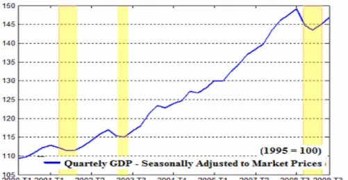
Figure 1: Quarterly Timeline of Brazilian Business Cycles.
In Figure 1, the shaded areas indicate periods characterized by recession. The dating of CODACE, considered recessions to be periods in which there was a sharp decline in the level of economic activity perceived for at least two consecutive quarters. The principal variable used in the dating of CODACE was the seasonally-adjusted quarterly gross domestic product (GDP) at market prices, calculated by the IBGE. Periods considered as recessions are respectively, from the second to the fourth quarter of 2001; from the …rst to the second quarter of 2003; and from the fourth quarter of 2008 onwards. According to the IBGE, the accumulated growth rates for these periods were 1%, 1:7%and 3:6%
respectively (the last …gure in the fourth quarter of 2008 alone). The …rst period considered as a recession refers to the second and fourth quarters of 2001. During this period, GDP fell for three consecutive quarters, caused principally by the energy crisis in Brazil, the attacks on the World Trade Center and the e¤ects of the bursting of the technology bubble in the United States. The recovery at the end of the year caused annual GDP to end with an increase of1:3%. The
second period considered as a recession refers to the …rst and second quarters of 2003. During this period, the Brazilian economy contracted by1:44%during the …rst quarter and by 0:23% in the second. In that year, however, GDP recovered and closed with an increase of1:1%. The causes were fundamentally the appreciation in the dollar which occurred in the preceding months due to the negative e¤ects of the sharp deceleration in the growth of the world economy on the renewal of credit lines for emerging countries and, in particular, of the expectations of economic agents regarding the management of the public sector debt by the Lula government, which took power in January 2003.
pub-lished on 28 December 2009, which was thus the largest average reduction since 1980. For the Committee, the resumption of expansion by part of industry, the sector most a¤ected by the crisis, is an indicator of the end of the recession. During this period, the crisis, which originated in the United States and was initiated by the US property market, caused instability in the …nancial markets and in the exchange rate, together with a declining trend in equity prices, [with these] representing elements which impacted the real economy, as they reduced the volume of productive investments. In its last report of 28 December 2009, CODACE stated, by using the GDP, production, sales, employment and income data that the period of recession in Brazil had ended, given that there was a trough in the Brazilian economic cycle during the …rst quarter of 2009. Accord-ing to the Committee report, the trough represents the end of a recessionary period and the start of a period of economic expansion.
3
The Dynamic Nelson-Siegel Model and
MS-VAR Representation of a three-factor model
The approach in Nelson-Siegel (1987) describes the yield curve through expo-nential weighting of the factors. In this approach, the proposed model is capable of representing a large number of maturities for interest rates as a mathematical function. The authors argue that these functions may be used to obtain a par-simonious model, representing the principal stylized facts, historically observed in the yield curve: monotonicity, convexity and a ‘bell’ shape, persistence of the level of interest rates, higher volatilities for short-term rates and low persistence ofspreads3 .The Nelson-Siegel representation of the yield curve is modi…ed in Diebold & Li (2006). The authors show that the above representation may be interpreted as a model of latent factors and 1t; 2tand 3tare the level, slope and curvature,
which vary over time, being weighted by a …xed component (factor loadings).
A change in the long-term factor, 1t , reproduces the same change in all of
the interest rates, regardless of their maturity. Diebold & Li (2006) identify this component for the US yield curve with a high degree of persistence, being associated with the in‡ation expectations of economic agents. In analogous fashion, an increase in the short-term factor, 2t , shall have an e¤ect more
predominantly on the short-term interest rates, a¤ecting the slope of the curve. Diebold & Li (2006) associate this factor with the expected behaviour of the economy, such as the expected level of economic activity. In this way, this component is directly related to economic cycles. An increase in the medium-term factor, 3t, will not immediately a¤ect long-term interest rates, but will
have a greater e¤ect on medium-term rates, indicating that the curvature of the yield curve will vary over time, reproducing the stylised fact of a ‘bell’ form of the yield curve.
It is also worth commenting that the factors 1t; 2t and 3t recovered
by Diebold & Li (2006) have a high degree of correlation with the empirical measures of level, slope and curvature which are commonly used4 . This result is highly desirable insofar as the methodology of Nelson & Siegel could not be considered appropriate if the factors deriving from it (which depend on the pre-speci…ed functional forms for the decay parameters) did not resemble the factors deriving from what economic agents understand by measures of level, slope and curvature, as set forth in Diebold, Rudebusch & Arouba (2006). In this way, the interest rates, observed as a time series, may be described jointly for the di¤erent maturities by the following regression model:
yt( ) = + 1 1t+ 2 2t+ 3 3t+ t (1)
fort= 1; :::; T: t ~N(0; )where is a diagonal matrix. The preceding
assumption implies that changes in interest rates of di¤erent maturities are not correlated.
In this regression model, is a constant for each maturity of interest rates and may be interpreted as a …xed e¤ect insofar as each constant re‡ects the particular characteristics for each maturity of interest rates which are observ-able and non-observobserv-able. In addition, despite the fact that within Brazil, the yield curve su¤ered a multitude of shocks during the selected period, altering its behaviour in terms of level and volatility, there is no loss of generality in assuming that the constant for every maturity, , does not vary over time, in addition to which, we avoid dictating a behavioural rule for the parameter, as well as the number of parameters to be estimated; 1t; 2t and 3t are the
factors which vary over time and j is the weight for the factorj and maturity
.
As made explicit in Diebold & Li (2006), the parameters j may be
con-sidered constant over time. In the work of Koopman, Mallee & Van der Wel (2008), using the monthly data of US Treasuryzero coupon bonds, provided by
Fama-Bliss, they argue that maintaining the decay factor …xed during the study period may be highly restrictive, since the slope factor 2t and the
cur-vature factor 3tare merely dependent on . Diebold & Li (2006) argued that
the gain for the adjustment and predictive power of the model is small when the decay parameter is allowed to vary.
If itis a vector of latent variables, it may be shown that its representation
may be made through vector autoregression (V AR) proposed in Diebold & Li
(2006). In this case, the dynamic of 1t; 2t and 3t may be described by a
V AR(1)model.
Pursuant to the account and according to Diebold & Li (2006), this struc-ture is already in a state space representation. According to Koopman , in an empirical study of the US yield curve, whose estimation methodology for the yield curve shall be adopted in this study, the factors which describe the same 4We de…ne the level as being the mean of all of the yields; slope as being the
have a long memory. Due to this fact, the process proposed by the authors of the factors is a random walk:
0 @ 12tt
3t
1
A=
0 @ 12tt 11
3t 1
1
A+
0 @ 12tt
3t
1
A (2)
for t = 1; :::; T: The initial conditions are 1 ~ N(0; ), diagonal,
and 1 ~ N(0; ); is not necessarily diagonal, i.e. the factor errors may
be simultaneously correlated. This process, proposed in Koopman (2007), is a particular case of the process proposed in Diebold & Li (2006). In this way, we may test whether the proposedV AR(1) may be reduced to a random walk for
the latent factors.
In order to estimate the yield curve described above, the approach used shall be the Kalman …lter, as used by Diebold, Rudebusch & Arouba (2006) and described in Koopman (2007). The authors implemented the simultane-ous estimation of the observation and transition equations, obtained the factor weights for each maturity and the dynamic between the factors which describe the interest rates. Diebold, Rudebusch & Arouba (2006) explain that single stage estimation is better because it is able to consider all of the uncertainties associated with the estimation of these parameters in a single step. De Pooter (2007), comparing various classes of the Nelson-Siegel model with monthly data for US Treasury zero coupon bonds of Fama-Bliss for the period from January 1984 to December 2003, found that the three-factor model with a decay parame-ter, , appearing and estimated in a single stage by the Kalman …lparame-ter, has a mean square error less than the same model estimated by two-stage least squares.
The Kalman …lter is an algorithm used for the linear prediction of the state vector, in this case, the latent variable vector, conditional on the observed vari-ables, interest rates. Under normality, the likelihood function of the model is obtained through the prediction error decomposition. Once the likelihood func-tion has been obtained, the coe¢cients are estimated by numerical methods. After the estimation of the parameters through the smoothing algorithm, it is possible to recover the smoothed state vector and to obtain some structural in-terpretation for these estimates. The likelihood function of the system depends on the prediction errors, their respective variances and the set of parameters,
= ( ; ; it; ; )and is given by:
L( ) =
T
X
t=1 1 2ln(2 )
1
2ln (jFt 1j) 1 2&
|
tjt 1F 1
t 1&tjt 1 (3)
where&tjt 1=yt( ) ytjt 1( )is the one-step forward prediction error and
4
Vector Autoregressive with Markovian
Switch-ing (MS-VAR)
TheM S V ARmodels arise from the union of two tools: V AR, introduced by
Sims (1980) and models which use Markov Switching to analyse the nature of regime changes in macroeconomic series, as developed by Hamilton (1989) on economic cycles in the United States. With this, it becomes possible to estimate
V ARmodels subject to regime changes.
In the analysis of time series, the introduction of the Markov Switching model is due to Hamilton (1988) and Hamilton (1989), with this latter study having inspired more recent contributions. The class of M S V AR models
provides a convenient structure for analysing multivariate representations with regime changes. These models permit various dynamic structures, depending on the value of the state variable,st, which controls the transition mechanism
between the various states. TheM S V ARmodel belongs to a more general class of nonlinear models that, conditional on a particular regime, the model is linear.
In this way, the M S V ARmodel may be described, pursuant to Krolzig
(2003), as an autoregressive process of observed time seriesyt= (y1t; y2t; :::; ykt)
the parameters of which are unconditionally variant over time, but constant when conditional on a discrete non-observed state (or regime) variable st 2
f1;2; :::; mg:
yt (st) =A1(st)[yt 1 (st 1)] +:::+Ap(st)[yt p (st p)] +B(st)ut (4)
where (st) =
8 > > > > < > > > > :
1= ( 11; :::; 1) ifst= 1
m= ( 1m; :::; m) ifst=m
; ut is a Gaussian
er-ror conditional on regimest:utjst~N ID(0; (st)): p is the order of theV AR;
m is the number of unobserved regimes and k is the dimensions of the
vec-tor of observed variables. Hence, this model may be described as being of typeM S(m) V AR(p):The transition functions in the matrices of parameters
(st); A1(st); :::; Ap(st)and (st)describe the dependence of theV AR
parame-ters in each regime. The important characteristic of a model with Markovian change is that the unobserved realisations of the regime st 2 f1;2; :::; mg are
generated by a discrete time stochastic process which may be represented by a Markov chain with …nite states5 , de…ned by its transition probabilities:
pjl= Pr(st+1=ljst=j) m
X
l=1
pjl= 1 8j2 f1;2; :::; mg (5)
5The di¤erence between the Markovian models and the models with a threshold
in which it is accepted that the Markov chain is irreducible and ergodic6 . In the model described by the equation (4) there is an immediate jump in the mean of the process after a regime change. It is frequently more probable to assume that the mean is modi…ed smoothly to a new level after transition from one regime to the other. In this situation, we may use a model with an intercept term,v(st), depending on the regime. We thus have:
yt=v(st) +A1(st)yt 1+:::+Ap(st)yt p+B(st)ut (6)
Constraining the linear V AR models and parameters which are invariant
over time, the mean form, adjusted by (4) and with the form of an intercept in (6) are not equivalent. These entail adjustment dynamics for the observed data, which are di¤erent after a regime change. While a permanent change in the regime by the mean (st) causes an immediate jump in the time series
vector observed for a new level, the dynamic response for a regime change in the intercept termv(st)is equivalent to a “shock” in the white noise seriesut:7
The inference with a view to dating regimes not observable in M S V AR
is made basically on the basis of the …ltering and smoothing of estimated prob-abilities.
The …ltering method is usually the algorithm of Hamilton (1989), but other …lters may be used, such as the Kalman …lter. Filtering permits inferences on the probability distribution of the non-observed regimest, given the information
setyt.
The EM algorithm is an approach broadly applied to the estimation by
maximum likelihood. The estimation procedure for the parameters is the max-imisation of the likelihood function and its use for inferences on non-observable states, st . This method nevertheless becomes less attractive as the number
of parameters grows. In this case, the EM, originally described by Dempter,
Laird & Rubim (1977) to recover missing observations from a normally distrib-uted sample is more appropriate. This methodology starts with estimates of omitted observations, and through iterative procedures, results in a new joint distribution which increases the probability of occurrence of a given observa-tion. The adaptation of this procedure to time series data was described by Schumway & Sto¤er (1982), also in a context of missing observations.
According to Hamilton (1989), the algorithm consists of two parts. In the …rst part, population parameters, including the joint probability density of the states, are estimated, and in the second part, probabilistic inferences are made on the unobserved states, using a non-linear …lter and smoother.
In this way, letstbe a given regime andYt 1= (yt 1; :::; yt p)the
endoge-nous variables used in the analysis. Considering that the erroruthas a normal
6There are various de…nitions of the term “ergodic”. For some authors, the …nite
prop-erty is that the initial state may be forgotten, for others that the mean converges over time independently of the initial state. In general, these de…nitions are not equivalent. Some de…n-itions exclude chains with transitory states having zero equilibrium probabilities. For further details, see Hayashi, 2000.
distribution and that the process is in the regimest =il in t, the conditional
density ofytis given by:
f(ytjst=il;Yt 1;!) = ln(2 ) 1=2lnj j 1=2exp yt yil
| 1 y
t yil
where il represents thel-th column of the identity matrixIN;yil =E(ytj
st = il;Yt 1is the conditional expectation of yt given that the process is in
il and ! is a vector which contains the population parameters, including the
autoregression parameters , and the transition probabilities governing the Markov chain of the unobserved states.
The information on the realisation of Markov states are collected in the vectorst, which consists of binary variables de…ned on the basis of a function
indicating each regime.
The conditional densities, for them possible regimes, are given below:
l= 2 6 6 6 6 4
f(ytjst=i1;Yt 1)
f(ytjst=im;Yt 1)
3 7 7 7 7 5
In order to obtain the marginal density ofyt two steps are followed, as set
forth above. In the …rst, the joint density ofytandst is written as a product
of the marginal and conditional densities. In the second, it is integrated with regard to all of the regimes. The results of the marginal density ofyt may be
interpreted as a weighted average of the conditional densities, where the weights are the probabilities of the regimes. In this way, we must make some inference on the unobserved regimes, via the BLHK (Baum-Lindgren-Hamilton-Kim) …lter and smoother, used in this work, which permits inferences on the process states through …ltered and smoothed probabilities.
The …nal results of theEM algorithm shows that the value of the likelihood
function increases with the number of iterations. At a determined …xed point for these iterations, the estimated parameters converge to the maximum likelihood estimators. In many studies using a regime change8 , the strategy adopted to determine the optimal number of regimes to be introduced into the model is based on economic theory and on stylised economic facts. Having chosen the optimal number of regimes, the standard tests ofV ARmodels (information criteria, likelihood ratio test or Wald test) may be used to choose the best model. There is a di¢culty in implementing tests for the choice of number of regimes: under the null hypothesis, some parameters cannot be identi…ed. In this way, the likelihood ratio tests (LR) do not have a standard asymptotic distribution and cannot be adopted9 .
Based on Hamilton (1989), we initially consider a model in the state space representation restricted to two regimes, where st = 1 indicates a recession
regime andst= 0 an expansion regime.
As discussed above, an economy may be considered to be in recession when its GDP falls for at least two consecutive quarters and vice versa. It should be noted that for the period analysed here, the state observe for the Brazilian economy predominantly corresponds to an expansion regime, even though it has shown a pattern which is informally termed “stop-go”. In other words, the Brazilian economy has alternated between low growth, or recession, and phases of accelerated growth, suggesting that we could adopt more than one form of classifying regimes. At the same time, within Brazil, there is no o¢cial disclosure by the Central Bank of business cycles within Brazil and only recently and uno¢cially by CODACE, and it is on the basis of these datings of CODACE that we shall evaluate the performance of our model.
In this way, the estimated model presents the following form, in which the …rst equation is of observation and the second of transition, so that for the representation of the state space we have:
yt = 1st+
2
styt 1+ stFt+Ut
Ft = st+ Ft 1+Nt (7)
where now yt = fyt(3m); yt(12m); yt(60m); 12gtg, yt( ) are the interest
rates for 3,12 and 60 months and 12gt the 12-month change in GDP;Ft =
fb2t; gtg and b2t are the estimated latent factors for the slope and gt is the
components of the trend in 12-month GDP growth rate; is a 4 2 matrix of weights,Ut, a vector of random components, which measure the movements
not captured by the model; st a vector of weights which portrays the e¤ects of
factors on the vector of interest rates and change in the GDP. By hypothesis, the factors are not correlated with the errorsUt for all of the lags. Nt ~ N(0; t)
and t is a diagonal variance and covariance matrix for the factors.
Each factor follows an unobserved autoregressive process in which all the parameters are functions of two distinct Markov processes, sb2t
t for the yield
curve factor ands gt
t for the economic factor. The Markov chains
b
2t
t represents
the rising phase (sb2t
t = 1) and the falling phase (s
b
2t
t = 0) in the securities
market, since the chain s gt
t represents expansion (stgt = 1)and recessions or
stagnation(s gt
t = 0)of the economic cycle. Given the hypotheses of the model,
the representation allows the process for the cycle in the securities market and for the economic cycle to be independent or unsynchronised over time.
5
Estimations and Results
5.1
Database
August 2009. Some descriptive statistics for the DI-Pré swap data are presented in Table 4, in the annex. Figure 7 shows the mean and median yield curve for the analysed period. The mean yield curve shows the normally observed behaviour, i.e. an increasing trend at maturity. The median yield curve shows ‡at behaviour (without a slope), an indication that during the analysed period, it is expected that the short-term rates will continue the same. I.e. it is expected that with regard to interest rates, economic policy will remain the same.
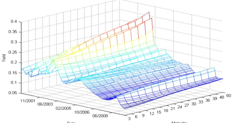
The yield curve for the study period considers various formats, with various changes in slope and curvature, assuming rising and inverted formats on various occasions during this period. Figure 2 shows a three-dimensional graph of the studied curve.
Figure 2: Brazilian Yield Curve - March 2000 to August 2009.
The analysis of the graph of Brazilian GDP shows a constant growth trend with falling periods, indicating a fall in economic activity during the period of analysis of this study. This behaviour may be seen with a monthly frequency, presented in Figure 1. The data refer to the series for Brazilian GDP during the period March 2000 to August 2009, calculated by the IBGE and published by the Brazilian Central Bank (BCB) (Series 4380).
However, according to the work of Chauvet and Senyuz (2009), we shall use the 12-month growth rate for GDP, set forth in Figure 3. For this series, the ADL and KPSS tests were carried out. In the ADL test, we reject the null hypothesis with a test statistic of 3:885509and a critical value of 2:8903at the 5% signi…cance level, indicating that this series is stationary. For the KPSS test, we do not reject the null hypothesis of stationarity, with a test statistic of
Figure 3: Monthly GDP growth – 12 month change
5.2
Results
In this section, the principal results are presented on business cycles in Brazil, using theM SIAH(2) V AR(1) class of models, for the real GDP 12-month
change data and the slope factor estimated by Kalman …lter, for the period from March 2000 to August 2009.
The parameters j and the factors jt were estimated by Kalman …lter.
Estimates were also obtained for the variance and covariance matrices and . For the identi…cation of all of the parameters j , the weights (factor
loadings) of the three factors for the maturities of3,12and60were restricted to
(1;0;0),(0;1;0)and(0;0;1), respectively. In this way, the maturity of3months is directly related to the slope factor. The maturities of12and60months were linked to the curvature and level factors respectively.
Figure 4: The weights estimated by Kalman …lter
As mentioned, the weights for the level factor are associated with longer maturities of48 and 60 months. The second and third factors are associated with the short and medium term maturities respectively. Observing the above …gures, the estimates for the weights of the second and third factors, slope and curvature, for the proposed model are very similar to the restricted weights proposed in Nelson-Sielgel (1987).
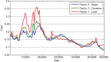
The smoothed estimates of the factors are presented in Figure 5.
Figure 5: Interest Rates - 3, 12 and 60 months
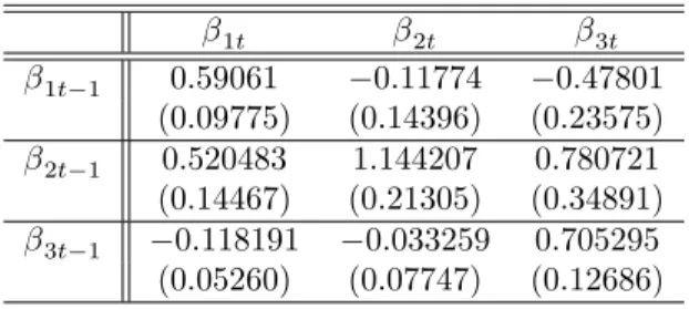
1t 2t 3t
1t 1 0:59061 0:11774 0:47801 (0:09775) (0:14396) (0:23575) 2t 1 0:520483 1:144207 0:780721 (0:14467) (0:21305) (0:34891) 3t 1 0:118191 0:033259 0:705295 (0:05260) (0:07747) (0:12686)
Table 1: Estimated Parameters of theV AR(1)for the Smoothed Latent Factors
(Standard Error in parentheses)
The autovalues of the matrix of coe¢cients of V AR(1) above are 0:5493,
0:9935 and 0:8973. Since one of the auto values is close to unity, the compo-nents of VAR are as a minimum integrated of order 1, and like the other two autovalues, are less than unity, with this indicating, together with the prior statement, that the components are at most integrated of order 1.
We propose a two-factor model, which takes into consideration the dynamic between the securities market and business cycles. This model uses the com-ponents of the yield curve to determine economic cycles with greater precision, analysing this through the 12-month growth rate of GDP.
Table 2: Parameters of the Model MS-VAR (1)
Observing Table 2 with the results of the estimation, we may see the dif-ferences between the two regimes. Comparing the variances of the variables, we may note that regime 1 has a lower variability of series than regime 0. In this way, Regime 1, for the expansion of the cycle, represents periods of low volatility, contrary to what occurs for Regime 0.
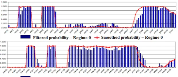
Figure 6: Filtered and Smoothed Probabilities for Brazilian Business Cycles
The MSIAH -VAR estimated above represents the following transition ma-trix:
T = 0:9836 0:0164 0:0341 0:9659
We thus perceive that estimated regimes are very persistent, i.e. once an economy is in a given regime, the probability of remaining within this regime is very high. In this way, the probability that the Brazilian economy is in a period of recession and will continue under the same regime for the following period is 98:36%; the probability that the Brazilian economy will be in a regime of cyclical expansion and will remain in it during the following period is 96:59%. The probability of shifting from a recessionary regime to an expansion regime is3:41% and the contrary probability is1:64%
Pursuant to the above probabilities, we may derive a time classi…cation of the regimes, presented in the following table. The duration of regime 1, an expansion regime, is approximately17 months, while the duration of 0, of recession or contraction, is approximately5 months.
For the interpretation of the graph, a probability of50% or lower indicates an expansion phase, while a probability exceeding 50% indicates a phase of recession or stagnation.
It may be seen in the graph with the …ltered and smoothed probabilities that the expansion regime(st = 1)holds for most of the analysed period, but
In accordance with the transition matrix, given that the economy is expand-ing or in a regime of recession, the probability that it remains under this regime is greater than of a change to the other regime. This indicates a lower ‡exibil-ity of transition between regimes, validating the slope of the yield curve as a relevant variable for economic cycles.
Pursuant to the presented result, since 2000, Brazil has shown relatively stable economic growth. There are no signi…cant divergences between the results of the model and the dating of the economic cycles drawn up by CODACE. This study nevertheless uses data with a monthly frequency, while the datings are drawn up on the basis of quarterly GDP. On average, the model pinpoints the peaks and troughs during the analysed period, but extends the last recessionary peak. It should be noted that the probabilities of a recession estimated by the model remained above 50% between 2008 and 2009. This does not invalidate the use of the slope component in the model. In fact, this is an expected fact, insofar as the Kalman …lter uses all of the available information for generating an optimal estimate for the factor.
6
Conclusion
We propose a model which captures information from the Brazilian yield curve for the evaluation of economic cycles: A multivariate model with 2 factors, slope and proxy for economic performance, which follows two Markov processes, each one representing the faces of the securities and asset markets. The results permit the direct analysis of the relationship between the cycle phases of these two sectors. The model is used for forecasting the start and end of recessions and expansions of Brazilian GDP with a monthly frequency. The results show a strong correlation between the economy and the securities market.
The adjustment showed itself to be close to the value expected from the datings by CODACE. In summary, the components of the yield curve, estimated by Kalman …lter, especially the slope factor, presents the information necessary for forecasting recessions and expansions of GDP growth.
Hence, the use of the factor estimated in a single step by Kalman …lter permits improvements in forecasting economic cycles in Brazil.
7
References
References
[1] Ang, A., Piazzesi, M., Wei, M. (2006) "What Does the Yield Curve Tell us About GDP Growth?".Journal of Econometrics,127, 359-403.
[3] Chauvet, M. Senyuz, Z. (2009) “A Joint Dynamic Bi-Factor of the Yield curve and the Economy as a Predictor of Business Cycles” mimeo.
[4] Dempster, A. P., Laird, N. M. Rubin, D. B. (1977) “Maximum likelihood from incomplete data via the EM algorithm”.Journal of the Royal Statis-tical Society,B,39, 1-38.
[5] De Pooter, Michiel. “Examining the Nelson-Siegel Class of Term Struc-ture Models - In-sample …t versus out-of-sample forecasting performance”. Technical Report 043/4. Tinbergen Institute.
[6] Diebold, F. Li, C. (2006) "Forecasting the Term Structure of Government Bond Yields".Journal of Econometrics,130: 337-364.
[7] Diebold, F., Rudebusch,G., Aruoba, S. (2006) "The Macroeconomy and the Yield Curve: A Dynamic Latent Approach".Journal of Econometrics,
131: 309-338.
[8] Estrella, A., Hardouvelis, G. A.(1991) "The Term Structure as a Predictor of Real Economic Activity,”Journal of Finance,46(2). 1.
[9] Estrella, A., Mishkin, F. S. “Predicting U.S. Recessions: Financial Vari-ables As Leading Indicators,” The Review of Economics and Statistics, MIT Press, Vol. 80. 1998.
[10] Garcia, R. “Asymptotic null distribution of the likelihood ratio test in Markov switching models”. Université de Montreal, working paper. 1993.
[11] Hamilton, J. D. “A new approach to the economic analysis of non-stationary time series and the business cycle, Econometrica”. 57, 357-384. 1988.
[12] Hamilton, J. D. “Analysis of time series subject to changes in regimes, Journal of Econometrics”. 45, 39-70. 1989.
[13] Hansen,B.E. “The likelihood ratio test under non-standard conditions: testing the Markov switching model of GNP”. Journal of Applied Econo-metrics. No. 7, p.61-82. 1992.
[14] Harvey, C., The Real Term Structure and Consumption Growth, Journal of Financial Economics 22, 305-334.
[15] Harvey, C., Forecasting Economic Growth with the Bond and Stock Mar-kets, Financial Analysts Journal, 38-45.University Press. 1989.
[16] Hayashi, F. Econometrics. New Jersey: Princeton
[18] Koopman, S.J., Mallee, M.I.P., Van der Wel. Analyzing the Term Struc-ture of Interest Rates using the Dynamic Nelson-Siegel Model with Time-Varying Parameters. Forthcoming in Journal of Business and Economic Statistics. 2008.
[19] Krolzig, H.M. “Business cycle analysis and aggregation. Results for Markov-Switching VAR processes”. Discussion Paper, Department of Eco-nomics, University of Oxford: 2003.
[20] Lima, A. M.C., Issler, J. V. “A hipótese das expectativas na estrutura a termo de juros no Brasil: Uma aplicação de modelos de valor presente” [The hypothesis of expectations in the term structure of interest rates in Brazil: An application of present value models] Economics Working Pa-pers (Ensaios Economicos da EPGE) 480, Graduate School of Economics, Getulio Vargas Foundation (Brazil). 2003.
[21] Marçal, E. F., Valls Pereira, P.L. “A Estrutura a Termo da Taxa de Ju-ros no Brasil: Testando a Hipótese de Expectativas Racionais” [The term structure of interest rates in Brazil. Testing the rational expectations hy-pothesis]. Pesquisa e Planejamento Econômico, 37, no 1, 113-147. 2007.
[22] Moolman, E. A. “Markov switching regime model of the South African business cycle.” Economic Modelling, v. 21, p. 631-646. 2004.
[23] Nelson, C.,Siegel,A. Parsimonious Modelling of Yield Curves. Journal of Business, 60: 473-489. 1987
[24] Sims, C. “Macroeconomics and reality”. Econometrica, v.48, 1: 1-48. 1990.
[25] Stock, J.H. and M.W. Watson, Forecasting Output and In‡ation: The Role of Asset Prices, Journal of Economic Literature, 41, 3, 788-829.2003.
[26] Stock, J., Watson, M. New Indices of Coincident and Leading Indicators, In O. Blanchard and S. Fischer ed. NBER Macroeconomic Annual, Cam-bridge, MIT Press.1989.
[27] Shumway, R.H.,Sto¤er, D.S. “An approach to time series smoothing and forecasting using the EM algorithm”. Journal of Time Series Analysis, 3, p. 253-264. 1982.
[28] Tabak, B.M., Andrade, S.C. “Testing the Expectations Hypothesis in the Brazilian Term Structure of Interest Rates,” Working Papers Series 30, Central Bank of Brazil, Research Department. 2001.
Table 2: Swap DI Pré - Descriptive Statistics
yt( 3 m ) yt( 6 m ) yt( 9 m ) yt( 1 2 m ) yt( 1 5 m ) yt( 1 8 m ) yt( 2 1 m ) yt( 2 4 m ) yt( 2 7 m ) yt( 3 0 m ) yt( 3 3 m ) yt( 3 6 m ) yt( 3 9 m ) yt( 4 8 m ) yt( 6 0 m ) M e a n 0 . 1 5 3 5 0 . 1 5 5 6 0 . 1 5 7 3 0 . 1 5 8 8 0 . 1 6 0 7 0 . 1 6 2 2 0 . 1 6 3 6 0 . 1 6 4 8 0 . 1 6 6 2 0 . 1 6 7 4 0 . 1 6 8 4 0 . 1 6 9 4 0 . 1 7 0 3 0 . 1 7 2 7 0 . 1 7 5 2 M e d i a n 0 . 1 5 2 1 0 . 1 5 5 8 0 . 1 5 5 9 0 . 1 5 6 9 0 . 1 5 8 4 0 . 1 5 9 2 0 . 1 5 8 8 0 . 1 5 7 6 0 . 1 5 7 9 0 . 1 5 7 2 0 . 1 5 6 7 0 . 1 5 8 8 0 . 1 5 6 6 0 . 1 5 5 5 0 . 1 5 7 2 M a x i m u m 0 . 2 4 2 9 0 . 2 4 8 4 0 . 2 5 7 4 0 . 2 6 9 3 0 . 2 8 0 8 0 . 2 9 1 1 0 . 3 0 1 1 0 . 3 0 8 0 . 3 1 5 0 . 3 2 1 8 0 . 3 2 7 5 9 . 4 9 4 0 . 3 3 7 5 0 . 3 5 1 2 0 . 3 6 5 5 M i n i m u m 0 . 0 8 2 5 0 . 0 8 3 4 0 . 0 8 5 2 0 . 0 8 8 0 . 0 9 0 7 0 . 0 9 2 2 0 . 0 9 4 2 0 . 0 9 6 5 0 . 0 9 8 9 0 . 0 9 8 6 0 . 0 9 8 1 - 1 2 . 1 1 1 0 . 0 9 7 7 0 . 0 9 7 2 0 . 0 9 6 7 S t a n d a r d D e v i a t i o n 0 . 0 3 7 0 . 0 3 9 6 0 . 0 4 1 7 0 . 0 4 3 6 0 . 0 4 5 7 0 . 0 4 7 5 0 . 0 4 9 2 0 . 0 5 0 7 0 . 0 5 2 5 0 . 0 5 4 1 0 . 0 5 5 5 1 . 5 4 4 0 . 0 5 8 0 0 . 0 6 1 2 0 . 0 6 4 5 A s s y m e t r y 0 . 2 9 4 2 0 . 3 5 3 1 0 . 4 7 4 8 0 . 6 1 1 8 0 . 7 3 9 8 0 . 8 5 1 2 0 . 9 4 5 4 1 . 0 1 9 6 1 . 0 7 1 5 1 . 1 1 4 6 1 . 1 4 7 - 0 . 6 1 1 . 2 0 0 8 1 . 2 5 4 6 1 . 2 8 1 3 K u r t o s i s 2 . 6 7 4 7 2 . 5 9 7 2 . 7 2 4 2 . 9 2 3 9 3 . 0 9 0 2 3 . 2 5 6 9 3 . 4 1 1 8 3 . 5 3 0 5 3 . 5 8 1 9 3 . 6 3 8 8 3 . 6 8 8 . 6 7 3 . 7 6 5 1 3 . 8 6 3 6 3 . 9 0 2 4 J a r q u e B e r a 2 . 1 4 6 7 3 . 1 4 0 8 4 . 6 4 4 5 7 . 1 3 8 2 1 0 . 4 3 8 5 1 4 . 0 7 8 3 1 7 . 7 8 9 2 1 . 0 9 0 4 2 3 . 4 2 4 6 2 5 . 5 4 1 8 2 7 . 1 9 1 6 3 6 4 6 . 2 7 3 0 . 1 7 7 4 3 3 . 4 4 7 3 3 5 . 0 6 1 1
P r o b [ 0 . 3 4 1 9 ] [ 0 . 2 0 8 ] [ 0 . 0 9 8 1 ] [ 0 . 0 2 8 2 ] [ 0 . 0 0 5 4 ] [ 0 . 0 0 0 9 ] [ 0 . 0 0 0 1 ] [ 0 . 0 0 0 0 ] [ 0 . 0 0 0 0 ] [ 0 . 0 0 0 0 ] [ 0 . 0 0 0 0 ] [ 0 . 0 0 0 ] [ 0 . 0 0 0 ] [ 0 . 0 0 0 ] [ 0 . 0 0 0 ] O b s e r v a t i o n s . 1 1 1 1 1 1 1 1 1 1 1 1 1 1 1 1 1 1 1 1 1 1 1 1 1 1 1 1 1 1 1 1 1 1 1 1 1 1 1 1 1 1 1 1 1
0.14 0.145 0.15 0.155 0.16 0.165 0.17 0.175 0.18
yt(3 m)
yt(6 m)
yt(9 m)
yt(1 2m)
yt(1 5m)
yt(1 8m)
yt(2 1m)
yt(2 4m)
yt(2 7m)
yt(3 0m)
yt(3 3m)
yt(3 6m)
yt(3 9m)
yt(4 8m)
yt(6 0m)
M aturity
Mean yield curve Median yield curve