www.atmos-meas-tech.net/8/4735/2015/ doi:10.5194/amt-8-4735-2015
© Author(s) 2015. CC Attribution 3.0 License.
High-resolution measurements from the airborne Atmospheric
Nitrogen Dioxide Imager (ANDI)
J. P. Lawrence1,a, J. S. Anand1, J. D. Vande Hey1, J. White1, R. R. Leigh1, P. S. Monks2, and R. J. Leigh1 1EOS Group, Department of Physics and Astronomy, University of Leicester, Leicester, LE1 7RH, UK 2Department of Chemistry, University of Leicester, Leicester, LE1 7RH, UK
anow at: Geospatial Insight Ltd, Coleshill, B46 3AD, UK Correspondence to: R. J. Leigh ([email protected])
Received: 1 April 2015 – Published in Atmos. Meas. Tech. Discuss.: 5 June 2015 Revised: 9 October 2015 – Accepted: 29 October 2015 – Published: 10 November 2015
Abstract. Nitrogen dioxide is both a primary pollutant with direct health effects and a key precursor of the secondary pol-lutant ozone. This paper reports on the development, charac-terisation and test flight of the Atmospheric Nitrogen Diox-ide Imager (ANDI) remote sensing system. The ANDI sys-tem includes an imaging UV/Vis grating spectrometer able to capture scattered sunlight spectra for the determination of tropospheric nitrogen dioxide (NO2) concentrations by way of DOAS slant column density and vertical column density measurements.
Results are shown for an ANDI test flight over Leicester City in the UK on a cloud-free winter day in February 2013. Retrieved NO2 columns gridded to a surface resolution of 80 m×20 m revealed hotspots in a series of locations around Leicester City, including road junctions, the train station, ma-jor car parks, areas of heavy industry, a nearby airport (East Midlands) and a power station (Ratcliffe-on-Soar). In the city centre the dominant source of NO2emissions was identified as road traffic, contributing to a background concentration as well as producing localised hotspots. Quantitative analy-sis revealed a significant urban increment over the city centre which increased throughout the flight.
1 Introduction
Statistical and epidemiological studies have linked atmo-spheric pollution in urban environments to health problems in humans (Latza et al., 2008). Recent studies estimate that the economic impact of poor air quality in the UK is as high as EUR 28 billion yr−1 (HoCEAC, 2011). In Germany, this
figure is even higher at EUR 33 billion yr−1 due to indus-trial emissions alone (EEA, 2011). Nitrogen dioxide (NO2) is an atmospheric pollutant abundant in urban areas owing to emissions from traffic exhaust, central heating systems and industrial activities. Correlations have been found be-tween the atmospheric concentration of NO2and respiratory symptoms, cardiovascular symptoms and hospital admis-sions (COMEAP, 2011). NO2is also a known tracer/marker for other combustion products such as sub-micron particulate matter (Wehner and Wiedensohler, 2003) and is a precursor for ozone formation (Monks et al., 2009).
Road transport is the largest contributor to urban NO2 con-centrations, and reductions of NO2(and NO) over the last 2 decades have not been as large as anticipated with NO2 lev-els being measured above legal limits at over 40 % of Euro-pean roadside air monitoring stations in 2010 (Carslaw et al., 2011). In the city of Leicester (UK), the focus region, ap-proximately 90 % of the atmospheric NO2is emitted by traf-fic, of which approximately 60 % is emitted by heavy goods vehicles and public transport, and like many cities in the UK Leicester is not meeting its European Commission regulatory limits on NO2concentrations (Davies, 2011).
to-pography of the urban landscape and the atmospheric chem-istry which occurs outside of the sensing volumes of the in situ monitors (CERC, 2003; Vardoulakis et al., 2007).
To gain perspective on the distribution of NO2around ur-ban environments, a remote sensing instrument known as the Atmospheric Nitrogen Dioxide Imager (ANDI) was de-veloped at the University of Leicester. The main compo-nent of the ANDI instrument is a compact imaging spec-trometer known as CompAQS (Whyte et al., 2009), which was installed in a light aircraft alongside a series of ancil-lary systems and flown in a push-broom nadir configura-tion on the 28 February 2013. When flown at 900 m alti-tude the ANDI system produces maps of NO2 differential slant column densities (dSCDs) beneath the aircraft across swaths approximately 600 m wide with an across-swath res-olution of approximately 5 m (see Sect. 2). The dSCDs are retrieved using the well-established differential optical ab-sorption spectroscopy (DOAS) technique (Platt and Stutz, 2008), which following post-processing involving a radia-tive transfer model to generate air mass factors (AMFs) con-verts them into vertical column densities (VCDs) in units of molecules cm−2. VCDs provide estimates for the NO2 con-centrations in vertical atmospheric columns having compen-sated for both viewing and solar geometries.
Aircraft are commonly used for testing and demonstrat-ing new instruments and retrieval techniques, particularly for flight demonstrators of satellite instruments. For atmo-spheric measurements of NO2in particular, aircraft open op-portunities for validation of atmospheric modelling activi-ties and have previously been used for validating satellite retrievals during intercomparison campaigns (e.g. Bucsela et al., 2008).
Imaging DOAS instruments which measure spectra across the nadir field of view have been previously employed in sev-eral flight campaigns (e.g. Heue et al., 2008; Popp et al., 2012; Schönhardt et al., 2014; General et al., 2014). As in the case of many satellite imaging instruments these oper-ate a push-broom viewing geometry, in which spectra from multiple nadir viewing angles across the flight track are im-aged onto the same charge-coupled device (CCD), which al-lows for high-spatial-resolution two-dimensional images of atmospheric pollution over the flight duration to be produced. These instruments are capable of imaging anthropogenic NO2distributions over heavily polluted regions, such as in-dustrial point-source emissions over the Highveld plateau in South Africa (Heue et al., 2008) and pollution originating from traffic in Zurich (Popp et al., 2012).
This paper describes the ANDI system and its test flight which focused specifically on the mapping of an urban ag-glomerate at very high spatial resolution. It is shown that with an appropriate flight plan, data collected by ANDI can pro-vide insight into both spatial and temporal urban NO2 dy-namics in a single flight, highlighting variability which is hidden to lower-resolution satellite measurements and in situ monitors.
Figure 1. ANDI instrument schematic showing main components: the red lines represent power connections, and the blue lines repre-sent communication connections.
2 The ANDI system
The ANDI system comprises of multiple subcomponents mounted on a rigid plate with two viewing apertures. The components include a CompAQS spectrometer (Whyte et al., 2009), the Global Positioning System (GPS), an inertial monitoring unit (IMU), a digital single-lens reflex (DSLR) camera and a power system to condition and convert the 28 V provided by the aircraft’s generators into the 12 and 19 V used by the ANDI instruments. The ANDI system design is shown in Fig. 1.
2.1 The CompAQS spectrometer
The CompAQS spectrometer was originally built as a tech-nology readiness improvement exercise towards the develop-ment of a compact grating spectrometer suitable for a small satellite mission (Whyte et al., 2009; Leigh et al., 2015). For application in the ANDI system the optical bench of Com-pAQS was modified and strengthened to allow for a vertical (nadir) configuration. In addition, the spectrometer’s shutter mechanism was replaced with a CCD frame transfer system. To minimise the transmission of vibration from the air-craft to the spectrometer and to protect the instrument from damage during landing, the spectrometer was mounted inside a secure metal frame using compressed foam as the fixing medium to prevent any hard contact between the spectrome-ter and the aircraft.
To mitigate the effect of electrical noise inherent in the production of power from the aircraft’s generators a power conditioning unit was installed in the main circuit between the ANDI’s power distribution hub and the aircraft’s 28 V power supply (see Fig. 1).
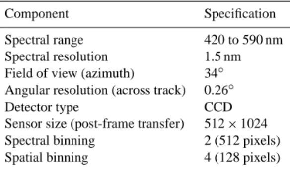
Table 1. Relevant specifications of the CompAQS spectrometer used in the ANDI system.
Component Specification
Spectral range 420 to 590 nm Spectral resolution 1.5 nm Field of view (azimuth) 34◦ Angular resolution (across track) 0.26◦ Detector type CCD Sensor size (post-frame transfer) 512×1024 Spectral binning 2 (512 pixels) Spatial binning 4 (128 pixels)
NO2 retrieval. The original design had a UV optimised grating (2350 grooves mm−1), while in ANDI a grating of 1800 grooves mm−1 was used for the fitting window speci-fied in Table 2. Additionally, in the Whyte et al. (2009) bread-board design a fold mirror was incorporated, which was re-moved in the ANDI iteration to simplify the design and to reduce internal stray light.
It is most likely that the degradation in the instrument line shape has occurred as a result of the build of the airborne ver-sion. Tolerances in the manufacture of the telescope mirrors, their mounts and the mounting on to the optical bench were not able to be compensated for; therefore the alignment of light incident on the entrance slit is not optimised.
The CompAQS spectrometer’s across-track field of view (FOV) is curved owing to the use of a two-mirror Schwarzschild entrance optics configuration (Leigh et al., 2015). To provide an appropriate viewing geometry for data analysis purposes the spectrometer was mounted such that the curvature of its FOV pointed towards the aircraft’s direc-tion of travel. The instrument’s FOV is approximately 34◦ spread over 128 pixels (600 m on the ground at 900 m al-titude). The aircraft travelled with an average velocity of 155 knots (80 m s−1), resulting in a forward spatial resolu-tion of approximately 80 m.
The along-track spatial resolution of the CompAQS spec-trometer is restricted by the maximum capture rate of the CompAQS CCD and its associated electronics. The capture rate during the test flight was approximately 1 Hz. This rate is defined as the total time between subsequent measurements; once the CCD has been exposed for a single frame (300 ms), charge is transferred to the covered storage areas. When this happens, the vertical clocks are stopped on the exposed por-tion of the CCD, and the data are processed (∼650 ms).
The CompAQS spectrometer measures spectra in the visible region of the electromagnetic spectrum which are converted into dSCD and VCD measurements of atmo-spheric NO2using the well-established DOAS technique (see Sect. 3.4 and 3.6). The specifications for the CompAQS spec-trometer in its airborne configuration are given in Table 1 and Sect. 3.4.
2.2 Attitude sensors
To relate the NO2measurements provided by CompAQS to a location on the Earth’s surface a GPS module was built based on a Parallax GPS chip, and software was written to extract the GPS sentences and convert them into longitude, latitude and altitude data with 1 s temporal resolution. In addition, an IMU was installed to provide banking data to compensate for changes in viewing geometry during the data analysis pro-cess. The IMU data were not used in the data analysis for the results presented in this paper owing to data corruption; therefore an alternative data source was derived to account for banking as described in Sect. 3.3.
3 Test flight and data processing chain
The ANDI system was installed and flown in a Cessna– Reims F406 aircraft on 28 February 2013 from 12:30 to 14:30 (GMT). The weather conditions were suitable for fly-ing the instrument but were non-ideal. The visibility in the boundary layer was slightly limited due to haze, and because of the time of year the solar elevation angle was between 26 and 30◦, resulting in a shallow light path for the slant col-umn measurements which rendered them susceptible to air mass factor uncertainties and spatial artefacts.
A flight plan was produced prior to the flight for operation at an altitude of 900 m with the sortie split into four sepa-rate stages: a flight along the M1 motorway to investigate pollution from fast moving traffic, a flight over Ratcliffe-on-Soar power station to observe stack emissions, a repeated flight along a main route through Leicester City to investi-gate the temporal evolution of NO2and a regular grid over Leicester City centre to investigate the spatial distribution of NO2over the city centre. The latter portion of the flight plan formed the longest component of the flight, requiring 13 tran-sects over the city centre to capture an area approximately 5 km×10 km.
During the flight the ANDI instrument was accompanied by two operators, one to monitor the spectra collected by the CompAQS spectrometer and one to monitor the DSLR and attitude data. All systems operated successfully through-out the flight except for a minor error with the spectrome-ter which occurred for approximately 46 s towards the end of the flight, leading to a gap in coverage over Ratcliffe-on-Soar power station.
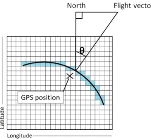
Figure 2. Schematic of the gridding process, showing the GPS loca-tion relative to the CompAQS field of view (curvature exaggerated for display purposes) shown as the black curve.
3.1 Data gridding
During the test flight, GPS provided longitude, latitude and altitude measurements at 1 s intervals. The first stage of the data gridding process involved allocating a GPS location to each measurement taken by the CompAQS spectrometer by running a nearest neighbour algorithm on their time stamps to synchronise the two data sets. The derivative of the GPS position data obtained from this process was then calculated to provide a direction of travel vector for the aircraft for each measurement throughout the flight.
Figures 2 and 3 present the geometry of the data gridding process and the variables which describe the orientation of the aircraft respectively. The relative position on the surface (in metres) of each pixel within the CompAQS FOV was as-signed based on the altitude of the aircraft, its position and its direction of travel at the time of the measurement using the GPS location to represent the centre of the instrument’s FOV (see Eqs. 1 to 6).
For consistency with the GPS data a non-regular spatial grid was defined in longitude/latitude coordinates with a spa-tial resolution of 20 m covering an area of 27×50 km. A search algorithm was used to fit each swath onto the grid, and any grid elements used more than once were averaged.
The calculation to determine the grid box locations for each surface pixel began with calculating the distance of each pixel from the centre of the instrument’s FOV both in the track and the along-track directions. In the across-track direction the distance (dik) from the centre of the in-strument’s FOV is given as
dik=aktan(φi+ψk) , (1)
where i is the index associated with an across-track Com-pAQS pixel, k is the index associated with each measure-ment swath,ais the GPS-derived altitude of the aircraft,φis
Figure 3. Schematic demonstrating the dimensions and geometry used to define the terms given in Eqs. (1) to (6).
the characterised CompAQS FOV angle for each pixel (see Fig. 3), andψis the banking angle of the aircraft calculated from the GPS data (see Sect. 3.3). In the along-track direc-tion the distancecfrom the centre of the instrument’s FOV is given as
cik=aktan(σi) , (2)
whereσ is the along-track angle of curvature of the Com-pAQS field of view for each pixel (see Fig. 3). In reality Eq. (2) would include an additional term to account for the pitch angle of the plane, but without reliable IMU data this could not be accounted for.
Using the results from Eqs. (1) and (2) the distance from the centre of the instrument’s FOV inxandycoordinates is computed using
xik=diksin(θk)+ciksin(±90±θk) , (3)
yik=dikcos(θk)+cikcos(±90±θk) , (4) wherexandyare the resultant pixel locations in metres from the centre of the instrument’s FOV, andθis the aircraft head-ing vector angle relative to north (see Fig. 2). Finally, ushead-ing the results from Eqs. (3) and (4), the latitude and longitude coordinates of each pixel are computed using
latik=
xik/Fklat
+GPSlatk , (5)
longik=yik/Fklong
+GPSlongk , (6)
Figure 4. Google Earth overlays of the raw intensity (442.7 nm) with 20 m resolution with (bottom) and without (top) along-track linear interpolation and 2×2 grid cell smoothing. The pixel coor-dinates derived in Sect. 3.1 were assumed to be the centre of the gridded data in the top plot.
GPSlatare the GPS position coordinates of the aircraft for a given swath in longitude and latitude, and long and lat are the final longitude and latitude coordinates of each pixel in the CompAQS field of view which are fed to the gridding algo-rithm. Note the±signs in Eqs. (3) and (4) dictate that either a+or a−should be used depending on the angular quadrant of the heading vectorθ.
The 5 m×80 m spatial resolution of the CompAQS spec-trometer resulted in significant gaps in the gridded data prod-uct at 20 m resolution. The pixel coordinates were also sub-ject to the temporal accuracy of the GPS chip (1 s) and so were approximations of their true location. To provide a spa-tially continuous data set, a linear interpolation algorithm was applied in the along-track direction of flight only, com-bined with a 2×2 grid box smoothing algorithm to aid in the identification of spatial features. Figure 4 presents an ex-ample of the effect of this process on the data, showing two data sets of raw intensity measurements from the test flight over the city centre at 442.7 nm before and after interpolation and smoothing. This smoothed data set is used in the analysis discussed later in this work.
Figure 5. Google Earth overlay of the CompAQS 442.7 nm forward interpolated intensity data showing co-location of bright industrial units and high intensity data recorded by CompAQS.
To determine the possible impact of the unknown bank-ing angle on this process the step change in GPS altitude per frame during the main phase of the flight (the Leicester City centre overpasses) was analysed to determine possible changes in the pitch angle. Neglecting the banking manoeu-vres, it was found that the actual measurement location was
±14 m away from the raw GPS position used in the grid-ding process. However, the frame rate of the CCD resulted in an average data gap of 90 m. Therefore, the captured frame would have always been positioned within the tolerance of the along-track resolution of the interpolated data set. 3.2 Data temporal synchronisation
Figure 6. Top: CompAQS 442.7 nm intensity data showing incor-rect georeferencing prior to banking corincor-rection. Bottom: CompAQS 442.7 nm intensity data showing improved georeferencing follow-ing bankfollow-ing correction. Two swaths are shown, one durfollow-ing bankfollow-ing (left) and one during level flight (right). Both swaths are overlaid on Google Earth.
3.3 Aircraft attitude compensation
Throughout the flight the aircraft’s necessary banking during manoeuvres introduced a variable FOV for the CompAQS spectrometer. To compensate for banking in the gridding pro-cess a data set of banking angles as a function of flight time was generated. These data would have been provided by the onboard IMU had the data not been corrupted; instead it was calculated by taking the temporal derivative of the aircraft’s bearing vector derived from the GPS data combined with a scaling factor. The magnitude of the scaling factor was deter-mined empirically by comparing the raw intensity measure-ments at 442.7 nm against bright surface features (see Fig. 6). The banking angle approximation would in future need to be replaced by the use of IMU data as the approximation’s ac-curacy cannot be guaranteed for all banking situations. 3.4 NO2retrieval
The NO2 differential slant columns were derived using the DOAS technique in a fitting window from 432 to 493 nm. The fitting window was selected to be reflective of similar studies, to permit fitting over a broad wavelength range and to minimise the fit RMS. A number of wavelength windows (approximately 20) were tested, with the final configuration selected, on the criteria above.
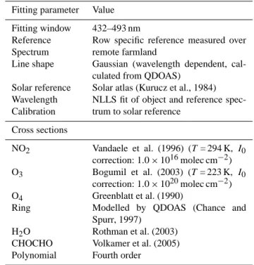
Table 2. Fitting parameters used for the DOAS fits in this work.
Fitting parameter Value
Fitting window 432–493 nm Reference
Spectrum
Row specific reference measured over remote farmland
Line shape Gaussian (wavelength dependent, cal-culated from QDOAS)
Solar reference Solar atlas (Kurucz et al., 1984) Wavelength
Calibration
NLLS fit of object and reference spec-trum to solar reference
Cross sections
NO2 Vandaele et al. (1996) (T= 294 K, I0 correction: 1.0×10¹⁶molec cm−2) O3 Bogumil et al. (2003) (T= 223 K, I0
correction: 1.0×10²⁰molec cm−2) O4 Greenblatt et al. (1990)
Ring Modelled by QDOAS (Chance and Spurr, 1997)
H2O Rothman et al. (2003) CHOCHO Volkamer et al. (2005) Polynomial Fourth order
The fitting routine was performed using the software QDOAS (Fayt et al., 2015). Included in the fit were cross sec-tions for NO2, O3, CHOCHO, O4, H2O and the Ring effect (Chance and Spurr, 1997), which were convolved with the wavelength-dependent Gaussian line shape calculated with the QDOAS software. These cross sections were also empir-ically corrected for the solarI0effect (Aliwell et al., 2002). A fourth-order polynomial was used to remove broadband structures, and no offset correction was applied. The fitting parameters are summarised in Table 2.
For this work no offset was fitted to account for spec-tral defects such as stray light. The removal of the offset within the DOAS fit did not substantially change the spatial structure in the VCD data but did marginally improve RMS-derived error estimates. An increase of approximately 20 % in the fitted NO2dSCD was observed. Future analysis should include a detailed examination of the impact of the offset fit-ting, particularly if extending analysis through to retrieval of surface volume mixing ratios.
Figure 7. Destriping procedure on the data from the ANDI instru-ment. In black are mean dSCD measurements from each across-track pixel, averaged over the entire flight. In red are mean dSCDs after destriping has been applied.
this, a wavelength-dependent shift and Gaussian line shape were calculated over the whole spectral window.
The reference spectra were measured at 12:33:56±2 s (GMT) over a region of farmland to the north of Leicester which was determined to have minimal influence from local emissions of NO2and therefore could be considered a uniform measure of background NO2for all across-track pixels. Errors on slant columns were calculated from the reduced chi-squared statistic of the DOAS fit (Fayt et al., 2015).
Data from the ANDI instrument exhibited striping on first analysis. This was likely caused by across-track defects in the CCD, spatially varying NO2within the reference region or differences in NO2sensitivity across the swath owing to changing instrument line shape. A correction was applied to remove this striping using all measurements recorded over Leicester City and surrounding rural areas (4500 along-track pixels). Data over Ratcliffe-on-Soar power station and East Midlands Airport were excluded to avoid any influence of significant discrete plumes. For each across-track pixel, a mean dSCD over the flight was calculated and a second or-der polynomial fitted across all of these values. Outputs from this process are shown in Fig. 7.
Over the entire flight, deviation from this polynomial curve was interpreted as a bias in the measurement from the across-track pixel in question. Therefore a correction factor was applied to adjust the mean dSCD value for each across-track pixel, so that the mean dSCD over the flight lay on this polynomial. The effectiveness of this process is demonstrated by the lack of striping in the final data set, despite signifi-cant inhomogeneity in NO2measurements. Such processes can only be applied when sufficient measurements are taken to ensure that a smooth polynomial can be assumed for the whole data set, and no dominant NO2sources are present in calculated means. The polynomial fitted includes AMF en-hancements to the dSCDs towards the edges of the swath, and this structure is retained in order to ensure VCD calcula-tions using AMF correccalcula-tions can be correctly implemented.
Variability in throughput and gain for each across-track pixel was corrected to ensure that calculations of surface albedo could be implemented across the swath. This correc-tion was calculated using data for the entire flight for the same wavelength used for the albedo calculations. A mean intensity for this pixel was calculated for the flight, and a correction factor applied to ensure that all across-track means were normalised.
3.5 Air mass factor computation
The dSCD measurements performed by the CompAQS spec-trometer are the result of an integrated light path from the Sun to the ground pixel and then to the instrument. When the solar elevation angle is small (as it is in February in the UK) the dSCD measurements are difficult to interpret as a final data product owing to the shallow light path; therefore VCDs were derived by computing AMFs. AMFs account for enhancements in the light’s atmospheric path length due to factors such as viewing geometry, aerosol scattering and sur-face albedo. Therefore, the VCD (Eq. 7) may be defined as the ratio of the SCD to the AMF (Solomon et al., 1987)
VCD= SCD
AMF. (7)
To compute the effects of atmospheric scattering the at-mosphere can be modelled as a set of altitude-resolved dis-crete layers. For optically thin species such as NO2the AMF can be generalised as the linear sum of the contribution of each vertical layer to the total SCD divided by the total VCD (Palmer et al., 2001; Boersma et al., 2004):
AMF= 6lml
ˆ b
xa,l
6lxa,l
. (8)
Here,ml is the box-AMF (BAMF), which represents the vertical sensitivity of layer l to NO2. Computation of the BAMF is performed using a set of forward model parame-ters, summarised by the term bˆ. These parameters include the scene viewing geometry, surface albedo, NO2profile and aerosol loading. Such parameters can either be derived from the instrument itself or determined from modelled data sets. An assumed a priori NO2profile,xa, is partitioned to calcu-late the VCD for each layer,xa,l. Computation of the BAMF requires the use of a radiative transfer model (RTM). Fur-ther discussion of the derivation of the AMF can be found in Rozanov and Rozanov (2010).
observa-Figure 8. A typical box air mass factor calculated by the SCIA-TRAN RTM for a rural ground pixel. The red line indicates the instrument altitude (0.9 km) at the time of the measurement.
tional geometry was provided using the positional data de-scribed in Sect. 3.1, while considerations for other forward parameters are discussed herein. An example of the vertical BAMF profile produced by the RTM is shown in Fig. 8. The AMF is mostly sensitive to conditions below the flight alti-tude, as the NO2and aerosol extinction profile chosen were at their largest below the boundary layer height.
A single NO2 profile used for the entire flight is shown in Fig. 9. The NO2profile was taken from the spatial mean profile over Leicester at 12:00 (GMT) on the day of the flight as forecast by the MACC-II model ensemble (Stein et al., 2012) and was modelled using a mean surface height of 0.0948 km. A high-resolution (5 m×5 m) digital elevation model (DEM) provided by BlueSky International Ltd. was used to correct for differences in local surface elevation as-sumed by MACC-II by scaling the profile to the DEM surface pressure using the technique explained in Zhou et al. (2009). The DEM data product provided by BlueSky International Ltd. did not include building topography. The effect of this on the retrieval is explored in the error analysis in Sect. 4.7.5. A single aerosol scenario was assumed during the flight, the mixing state for which was defined using the World Me-teorological Organization (WMO) database (Bolle, 1986), which assumes particle size distributions and spectral refrac-tive indices for six components of atmospheric aerosol: water soluble, dust, oceanic, soot, stratospheric and volcanic. Ta-ble 3 presents a summary of the scenario used in the AMF computation.
By applying the aerosol backscatter gradient method sim-ilar to that described by de Haij et al. (2009) to data from a Campbell Scientific CS135 ceilometer located at 52.7814◦ (lat.),−1.2844◦(long.), the boundary layer height during the flight was estimated at 0.7 km, which has been reflected in the lowermost aerosol layer height in Table 3. For all
scenar-Figure 9. The mean MACC-II NO2profile forecast over Leicester at 12:00 (GMT) on 28 February 2013. The boundary layer profiles assumed in this work are shown in Fig. 17.
Table 3. The aerosol loading scenario based on the WMO climatol-ogy assumed for all ground pixels in this study.
Layer height (km) Mixing state
0.0–0.7 urban 0.7–20.0 continental 20.0–50.0 background 50.0–100.0 background
ios the aerosol extinction profile was modelled as constant up to the boundary layer height and then exponentially decaying with height afterward (scale height: 0.2 km). This profile was scaled to the mean aerosol optical depth (AOD) at 469 nm of 0.0798 forecasted over Leicester at the time of the flight by MACC-II.
re-moved through the use of an empirical correction factor for each ground pixel. The correction factor was calculated by first computing the expected intensity at 442.7 nm based on all forward model parameters using SCIATRAN for each ground pixel for scenarios with and without aerosol loading. The ratio of the two modelled intensities is then multiplied by the raw intensity measurement to generate an intensity data set with reduced aerosol influence.
Following the aerosol correction, the surface albedo of each ground pixel was approximated by linearly scaling the corrected surface intensities recorded by the spectrometer at a single wavelength (442.7 nm) between two reference albedo values. The intensities recorded over regions with wa-ter (albedo: 0.07; Clark et al., 2007) and white roofs (albedo: 0.56; Baldridge et al., 2009) were used as the references. For this method to be valid it is assumed that the sensitivity of the CompAQS CCD across the fitting window is correctly represented by 442.7 nm. In the absence of characterisation data for the CompAQS CCD the accuracy of this approxi-mation cannot be determined; however, a visual inspection of the intensity data across the fitting window did not reveal any significant sensitivity bias which would suggest the ap-proximation is inappropriate.
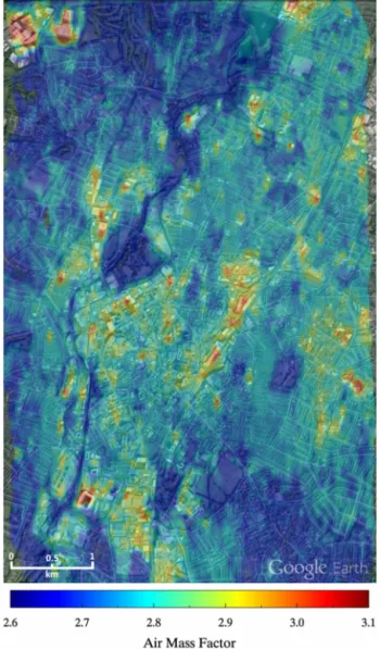
A gridded data set of the AMFs computed for this work is shown in Fig. 10. The variability present in the data set is dominated by surface albedo, with bright surfaces (e.g. white roofs) coinciding with high AMFs and darker regions (e.g. parks, a canal/river) coinciding with lower AMFs. This is consistent with previous investigations (e.g. Boersma et al., 2004), in which the AMF is also shown to be most sensi-tive to surface albedo in the absence of clouds and significant variations in the NO2profile.
3.6 Vertical column density computation
To calculate VCDs from the ANDI dSCD measurements it is necessary to account for tropospheric and stratospheric NO2 present in the DOAS reference region. The diurnal increase in stratospheric columnar NO2 has been previously esti-mated to be approximately 1.0×10¹⁴molec cm−2h−1 (Suss-mann et al., 2005), which is negligible in comparison to the VCDs retrieved which were on average approximately 3.5×10¹⁶molec cm−2. Therefore, it may be assumed that the stratospheric vertical column over the flight region re-mained approximately constant.
In a similar experiment involving imaging NO2from air-craft, Popp et al. (2012) attempted to correct for reference region tropospheric NO2in the retrieved dSCDs by adding a single offset estimated from previous air quality model stud-ies (Huijnen et al., 2010). For the spatial scales covered in this work, however, this approach is unsuitable owing to the coarse spatial resolution offered by such models in compar-ison to the small region analysed. Instead, the dSCDs mea-sured by ANDI are treated as the NO2increment above the lowest dSCD measured throughout the flight, implying the
Figure 10. The gridded AMFs calculated for this work, overlaid on Google Earth, showing the sensitivity of the AMF computation to surface albedo. Bright regions such as white roofs result in higher AMFs, while darker regions such as rivers, canals and parkland have lower AMFs.
VCDs calculated from the flight are defined as the incre-ment above UK background levels on the afternoon of the 28 February 2013.
4 Results
The test flight was divided into four components: three spa-tial regions, Leicester City centre, the M1 motorway and Ratcliffe-on-Soar power station, and a study on the temporal variability of NO2 over Leicester City centre. The findings from each of these components are covered separately in the following sections.
back-Figure 11. NO2VCD data recorded over Leicester City centre over-laid on Google Earth with areas of interest highlighted. Regions of interest labelled in the diagram are the train station (1), industrial areas (2), car parks (3), farmland (4) and highly emitting roads and junctions (5).
ground site. Therefore, independent verification of the ANDI data was not possible in this work. Instead, relative compar-isons between the regions were made to show that ANDI can retrieve the spatio-temporal variations in NO2 over the re-gion.
However, the VCDs in this work are themselves relative to the background rural NO2 present at the reference re-gion when the reference spectra were measured. The degree of this offset cannot be accurately estimated at the time of this work, but analysis of satellite-derived tropospheric NO2 VCDs from the Ozone Monitoring Instrument (OMI; Levelt et al., 2006) over Leicester measured during February 2013 suggest that the background column could be between 0.1 and 0.8×10¹⁶molec cm−2. The presence of this unknown offset will have an impact on the relative differences calcu-lated herein, so it is assumed that the background offset is the same over all regions, such that the VCDs measured in this work are the “urban enhancement” due to local emissions.
4.1 Leicester City centre
The main component of the ANDI test flight consisted of a series of 13 transects flown over Leicester City centre be-tween 12:43 and 13:43 (GMT). From the ANDI data a map of NO2VCDs was generated as shown in Fig. 11.
The VCDs recorded over Leicester City centre were mea-sured to be on average∼4.0×10¹⁶molec cm−2, approxi-mately 0.65×10¹⁶molec cm−2 (20 %) higher than in two of the city’s suburban areas (see Fig. 13 and Table 5 for where these areas are defined). Contributing factors for this enhancement are road traffic and a number of discrete emis-sion sources within and around the city centre, including high VCDs around the train station (1), industry (2), heavily used car parks such as supermarket and cinema car parks (3) and some particularly highly emitting roads and junctions (5) (see Fig. 11). The NO2 VCD hotspots observed by ANDI were associated with various sources by identifying the land use directly beneath them. Any hotspots that were not easily as-sociated with a particular source were not labelled in Fig. 11; however these sources are likely associated with road traffic as they are over areas where there are no obvious sources of industry or combustion activity.
Comparison of air masses in the city centre region (de-fined as region (c) in Fig. 13) with air masses which reside in the absence of busy roads and junctions such as over ar-eas of vegetation and agriculture (4) provide an indication of the urban increment of atmospheric NO2 for Leicester City centre. An area of particularly low NO2VCDs is given as region (a) ii in Fig. 13 and Table 5 where there are very few roads and no sources of industrial activity. The city centre (region c) has a 1.04×10¹⁶molec cm−2 (36 %) higher av-erage VCD than region (a) ii; the majority of this increment is likely associated with Leicester’s road traffic for reasons discussed.
A positive trend in atmospheric VCDs of 0.49×10¹⁶molec cm−2h−1 was measured over the city centre region from 12:43 to 13:43 (GMT), of which at least 0.23×10¹⁶molec cm−2h−1 has been identified as temporal in nature (see Sect. 4.4). Consequently the comparisons made between the city centre and other regions are only applicable to the time when the measurements were made. For the city centre (region c) the measurements were performed at approximately 13:10 (GMT).
Figure 12. Schematic showing the contribution of solar geometry to the north–south striping seen in the data. Plumes 80 m high will produce 150 m artefacts on the surface.t1andt2correspond to two measurement intervals 150 m apart.
exaggerated by an additional pitch angle introduced by the ANDI instrument being misaligned on the aircraft so that it did not have an exactly nadir-centred viewing geometry.
The striping behaviour appears to be repeated in the AMF data in Fig. 10, though it does not appear as prevalent in the VCD data in Fig. 11. The albedo data were derived from the intensity data, so it is expected that the AMFs would exhibit similar behaviour. Figure 11 suggests that the albedo deriva-tion has helped to at least partially account for this effect, but in future flights a functioning IMU would help to more precisely account for this effect.
The VCDs observed during the banking manoeuvres to the north-east of the city (see Fig. 13) at the end of each transect also show considerable enhancement, which does not cor-respond to known emission sources. The enhancement seen over that region is similar to those observed over the other banking manoeuvres during the flight, so it is possible that this is due to a large path length enhancement caused by a change in the roll angle. This would explain why the largest VCD appears to be at the outer edge of the swath, corre-sponding to the longest path length observed. As the IMU data were corrupted it was not possible to adequately include these effects in the AMF computation, which may lead to fea-tures such as this appearing in the final data set. It is likely that such features will not have appeared if the IMU was op-erational, and we envision that subsequent flights will not be subject to these effects.
4.2 M1 motorway
To investigate the contribution of the M1 motorway to local air quality the ANDI instrument was flown along a 24 km length of the M1 between 14:18 and 14:28 (GMT). Figure 13 highlights this component of the flight using two “M1” in-dicators. Towards the end of the M1 measurement region in the vicinity of Ratcliffe-on-Soar power station and East Mid-lands Airport (EMA), the VCDs became dominated by high
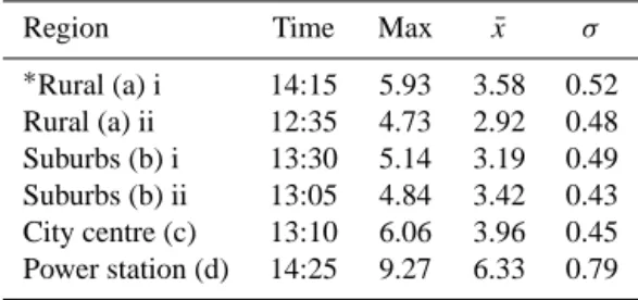
Table 4. VCD max, mean (x¯) and standard deviations (σ) in (molec cm−2 ×10¹⁶) from selected areas within the ANDI gridded data (see Fig. 13).∗Rural (a) i is an anomaly discussed in Sect. 4.6. The times presented are the approximate measurement times for each region.
Region Time Max x¯ σ
∗
Rural (a) i 14:15 5.93 3.58 0.52 Rural (a) ii 12:35 4.73 2.92 0.48 Suburbs (b) i 13:30 5.14 3.19 0.49 Suburbs (b) ii 13:05 4.84 3.42 0.43 City centre (c) 13:10 6.06 3.96 0.45 Power station (d) 14:25 9.27 6.33 0.79
concentrations (see Figs. 13 and 14). This region of high NO2 is likely associated with emissions from the power station and the airport. Before this area, however, there is no dis-cernible NO2signal originating from the motorway. This re-sult may be due to low traffic volumes during the overpass as is indicated by the visible imagery captured during the flight, as well as good venting of the area owing to the exposed na-ture of the M1 motorway.
4.3 Ratcliffe-on-Soar power station
Ratcliffe-on-Soar power station is a 2000 MW coal-fired power station 4.8 km from EMA, 9.7 km from Nottingham City centre and approximately 24 km from Leicester City centre. During the final few minutes of the test flight ANDI was flown directly over the power station to assess the magni-tude and extent of its emissions. However, the spectrometer abruptly failed for 46 s during the overpass, which resulted in a gap in coverage. Figure 14 presents the ANDI VCD data for this area with an appropriate colour scale to identify struc-ture in the NO2concentrations near to the power station and EMA.
Table 4 summarises the average VCDs measured from six regions of interest (two rural regions, two suburban regions, the city centre and the power station) to put the NO2VCDs in these areas into context with the power station and each other.
de-Figure 13. Complete ANDI data set from the test flight plotted in Google Earth with features of interest and areas used for regional averages highlighted. Coordinates for these regions are provided in Table 5. The gap in the data just prior to the power station is caused by the CompAQS spectrometer failing for 46 s. The single scans downwind of the power station are from the instrument temporarily stopping and starting because of an issue with the control software.
Figure 14. Google Earth overlay of NO2VCDs over Leicester and an area close to Ratcliffe-on-Soar power station and EMA. The colour scale is appropriate to discern structure within the area. The emissions from the power station are likely elevated having been emitted from a 200 m high chimney. The gap in the data just prior to the power station is caused by the CompAQS spectrometer fail-ing for 46 s. The sfail-ingle scans downwind of the power station are from the instrument temporarily stopping and starting because of an issue with the control software.
termine the full extent of the plume or suitably identify the origin; therefore a future study may include a more
exten-sive survey of this region and further consideration of how a plume aloft can be separated from surface concentrations.
It should be noted that the NO2 emitted from Ratcliffe-on-Soar power station is released into the atmosphere from a 200 m high chimney stack. ANDI measures VCDs and there-fore the vertical distribution of the power station emissions must be taken into account if surface concentrations are to be derived from these data. Additionally, the stack height influ-ence was not accounted for in the static vertical profile used in the AMF computation, possibly further biasing the VCDs observed here.
Despite the difference in vertical profiles, the elevated VCDs observed over the power station show that ANDI is capable of resolving point emission sources above the local background.
4.4 Temporal variability of NO2VCDs
Figure 15. Google Earth overlay of the repeat NO2measurements over Narborough road and the A6 moving through time from top to bottom. Each point on adjacent transects is approximately 6 min apart. Coordinates for the region are provided as region 1 in Table 5.
4.5 Regional summary
The results demonstrate both a temporal and spatial consis-tency in NO2VCDs throughout the 20 min the measurements were taken. On the left side of the transects (region A of Fig. 15) there is a temporally consistent area of relatively high NO2 VCDs which coincides with industrial buildings and a major road junction leading onto the M1 motorway. Between this junction and Leicester City centre (region B) there is a temporally consistent area of relatively low NO2 VCDs over an area of Leicester’s suburbs. Towards the mid-dle of each transect (region C) there is a relatively high area of NO2VCDs which is Leicester City centre, with a small but highly discrete area of relatively very low NO2 VCDs near to the middle (region D). The area of relatively low NO2VCDs in the city centre is present in all four transects (though less obviously in the first and last transects); how-ever its exact position and magnitude varies, which may be associated with a combination of meteorological and emis-sion variability and to some degree georeferencing error on account of aircraft banking uncertainty, GPS precision and measurement location variability on account of ANDI’s 80 m forward spatial resolution. The surface type beneath region D is parkland (Abbey Park), demonstrating the presence of a stable air mass with relatively few emissions beneath it.
From these qualitative observations it may be concluded that single instances of NO2VCD measurements are suitable for characterising the approximate spatial distribution and relative magnitude of a city’s atmospheric NO2 concentra-tions on a regional urban scale (> 1 km). However, the
tempo-Table 5. Coordinates for regions of interest the top 6 region identi-fiers are associated with Fig. 13, region 1 identifier with Fig. 15 and region 2 identifier with Table 6. (a) Rural areas, (b) suburban areas, (c) city centre area, (d) power station area.
Region Long. low Long. high Lat. low Lat. high
(a) i −1.292 −1.168 52.508 52.535 (a) ii −1.226 −1.186 52.672 52.706 (b) i −1.117 −1.092 52.606 52.627 (b) ii −1.146 −1.123 52.663 52.682 (c) −1.146 −1.120 52.630 52.648 (d) −1.337 −1.204 52.846 52.914 1 −1.134 −1.132 52.645 52.646 2 −1.161 −1.158 52.617 52.620
ral and spatial variability observed for Abbey Park (region D) demonstrates that significant over- or underestimation of at-mospheric concentrations of NO2could occur at finer spatial scales (< 1 km) if an individual measurement is attributed to average conditions, particularly where there are strong and potentially intermittent sources. This is also a reminder that these measurements are total column in nature and do not inform on the surface concentrations directly.
Figure 16. VCD measurements as a function of measurement index (time) with line of best fit presented in red. Measurements were averaged over±30 pixels from the nadir, taken from 12:43 to 13:43. Line gradient is 0.49×10¹⁶molec cm2h−1
Figure 17. The constant (red) and exponential (blue) boundary layer NO2profiles used in the perturbation study. Above 2 km the profile is the same as Fig. 9 (black). The dashed line represents the average flight altitude (900 m).
how this change might impact the AOD and in turn the AMF, the OPAC aerosol model (Hess et al., 1998) was used to esti-mate the impact with a continental average aerosol configura-tion. The results showed that an increase in RH from 50 % to 60 % would lead to an 8 % increase in AOD at 450 nm. How-ever, as is shown in the perturbation study in Sect. 4.7.4, a 20 % increase in AOD was calculated to change the retrieved NO2 VCD by less than 1 %. Therefore, given the informa-tion available, the 6.4 % increase in NO2during this portion of the flight appears to be associated with an increase in at-mospheric NO2, possibly as a result of emissions build-up in the atmosphere owing to slow wind speeds during the flight (1.2 m s−1 on average) combined with oxidation chemistry of NO to NO2.
Table 6. Average VCD measurements in molec cm−2 ×10¹⁶for region 2 in Table 5 for five overpasses.
Measurement time NO2VCD
12:40 3.75 13:43 3.94 13:49 4.01 13:54 3.94 14:01 4.11
To separate the temporal from the spatial (east to west) contributions within the observed VCD gradient, a region of interest (defined as 2 in Table 5) was averaged for five time intervals where spatial coincidence was achieved throughout the flight, thus obtaining NO2measurements without signif-icant spatial variability. The results are presented in Table 6. The first data point of the five available was measured during the first overpass of region (c) in Fig. 13, which was 1 h prior to the following four data points which were taken during the repeated flights across Narborough Road and the A6.
The temporal gradient in the VCD measurements from the five data points is approximately 0.23×10¹⁶molec cm2h−1, confirming the existence of a temporal increase in NO2 con-centrations throughout the flight. The difference in magni-tude between this result and the temporal trend over the city centre (0.49×10¹⁶molec cm2h−1) may be partially ex-plained by the location of the region sampled, which was sub-urban and therefore will have lower NO2emissions than the city centre. In addition it must be considered that the data used for the latter study were very sparse both temporally (only five data points) and spatially (only 220 m×220 m area) and therefore subject to significant uncertainty on ac-count of local spatial and temporal variability in atmospheric composition and emission sources (see Fig. 15) as well as statistical error. In addition, the ANDI surface pixel locations differ from scene to scene within the region of interest which could also have led to differences in the results.
With recognition of the significant uncertainties in-volved in quantifying and characterising the VCD trend over the city centre, it may be concluded that at least 0.23×10¹⁶molec cm2h−1 (47 %) of the NO2 trend is the result of a temporal increase in the atmospheric concentra-tion of NO2over the city centre.
4.6 Spatial distribution of NO2VCDs
Table 7. Perturbation study results showing absolute and relative mean uncertainties (±δx¯), maximum uncertainties (±δmax) and standard deviations (±δ σ) for five perturbation scenarios. The NO2profile shape study involves two alternative profile shapes (see Fig. 17); the results for each are presented in the+perturbation cells only. The units of the absolute uncertainties are in molec cm−2.
Parameter Perturbation +δx¯ ×1013 −δx¯ ×1013 +δmax×1014 −δmax ×1014 +δ σ ×1013 −δ σ ×1013
Albedo ±0.02 −14.1 (−2.4 %) 18.3 (2.8 %) −17.6 (−6.6 %) 9.7 (1.4 %) 11.3 (0.57 %) 11.9 (0.21 %)
AOD ±20 % 6.23 (0.90 %) −5.8 (−0.82 %) 9.06 (3.05 %) −8.8 (−2.51 %) 8.51 (0.22 %) 8.29 (0.27 %)
DEM ±10 m −1.5 (0.26 %) −1.91 (−0.34 %) 3.89 (2.29 %) −3.13 (−0.72 %) 2.12 (0.12 %) 2.57 (0.14 %)
NO2Profile exponential −13.4 (−1.9 %) n/a −17.2 (−3.64 %) n/a 18.7 (0.48 %) n/a
NO2Profile well mixed −41.7 (−6.5 %) n/a −49.8 (−8.22 %) n/a 59.6 (1.7 %) n/a
accumulation of multiple emission sources over time asso-ciated with a particular region appear to contribute to spa-tially extensive regional biases in atmospheric NO2 concen-trations. The finer-scale variability (< 1 km) is present in both Figs. 11 and 15, in which individual sources likely in com-bination with local meteorology appear to influence the local magnitude and distribution of the atmospheric NO2 concen-trations. In the context of human exposure, consideration of both scales is important, as the large-scale variability demon-strated by the temporal trend discovered over the city centre (see Fig. 16) will modulate the finer-scale distributions which are of interest where concentrations may exceed legislated safe limits.
Repeat flights along Narborough Road discussed in Sect. 4.4 demonstrated the presence of a temporal compo-nent to the NO2 VCD trend observed over the city centre; however, a contribution from an east–west spatial trend can-not be discounted.
Along-track spatial biases introduced by the low solar el-evation angle and along-track spatial interpolation were po-tentially contributing factors to the partial disappearance of the area of low NO2VCDs in the vicinity of Abbey Park in the top and bottom transects of Fig. 15. In addition, wind is likely to have also contributed to the differences observed in the transects, particularly over the Abbey Park area which may have been subject to import of NO2from the surround-ing road network. The wind speed measured by the Leices-ter City Council meteorological station (lat. 52.652◦, long.
−1.176◦) was approximately 1.2 m s−1 at 15◦ from north, which varied by < 0.2 m s−1 and 5◦ from north during the flight. The contribution of the wind vector to the spatial dis-tribution of atmospheric NO2is difficult to discern in the data sets owing to the spatial artefacts discussed previously and the low wind speed.
Region (a) i in Table 5 and Fig. 13 highlights an anomalous region of high NO2VCDs which is difficult to attribute to a particular source. The surface beneath region (a) i is farmland with only a single source of industry in the form of a small farm machinery factory and no additional sources of industry or major roads within a 1.6 km radius of the area. Despite the apparent scarcity of sources, the measured VCDs over this area are of a similar magnitude to Leicester City centre.
4.7 Uncertainty analysis
The error in the retrieved VCD measurements is a combina-tion of the uncertainties in both the dSCD and AMF calcula-tions.
The mean dSCD error across the flight can be calculated from the DOAS fit process. The mean dSCD over the flight was 1.9×10¹⁶molec cm−2, while the mean error calculated from the DOAS fit was 7.0×10¹⁵molec cm−2(37 %).
The uncertainty in the AMF computation is more difficult to determine. An approximation for the uncertainty of some of the independent parameters associated with the AMF have been derived by means of a perturbation analysis. The results of the perturbation analysis are discussed for each parameter herein, with Table 7 presenting a summary of the uncertain-ties derived from the study.
4.7.1 Methodology
The uncertainties associated with the forward model parame-ters used to produce the AMFs are more difficult to quantify, as each parameter contributes to the overall error budget and in many cases the individual errors are unknown. To provide a simplified estimate for the retrieval uncertainty associated with the AMF computation, a perturbation analysis was per-formed and is presented in this section. It is assumed the in-dependent parameters for the AMF are uncorrelated (i.e. their effects are independent of each other). Each forward model parameter in turn was perturbed by an error estimate result-ing in perturbed AMF and VCD values for all ground pixels. The resulting VCDs were subsequently compared against the original VCDs, and the resulting difference was calculated based on the mean deviation from the original values over the entire flight. The VCD modulations caused by the pertur-bations are representative of a constant bias in the perturbed parameter throughout the flight and therefore provide an esti-mate for the relative importance of each independent param-eter. The details of the parameters perturbed are discussed herein.
the magnitude of the uncertainty associated with this omis-sion, the DEM height used for each ground pixel was per-turbed by±10 m, which is approximately the mean building height in Leicester.
According to the MACC-II validation report for Febru-ary 2013 (Eskes et al., 2013) the modelled AOD at 469 nm over England had an average bias of−20 % when compared with AERONET data. The AOD was therefore perturbed by
±20 % for this study. Additional sources of potential error associated with aerosols not accounted for in this study were the vertical profile of the aerosols and their single scatter-ing albedo. It has been found that these factors can influence the sensitivity of the retrieval to NO2below or within such aerosol layers (Leitão et al., 2010). For this work, no mea-surements that would yield information on such factors other than the boundary layer height were available, and therefore error estimates of these properties could not be reliably de-fined.
A previous study has shown that uncertainties in the NO2 profile shape can lead to AMF uncertainties of approximately 10 % (Boersma et al., 2004). It is assumed in this work that the stratospheric NO2 concentration is approximately con-stant throughout the flight; therefore the NO2 profile un-certainty may be considered to be entirely associated with the correctness of the boundary layer NO2 profile compo-nent only. To obtain an approximation for the influence of boundary layer NO2 profile shape uncertainty on the VCD results, the MACC-II profile was altered to form two scenar-ios which would make sensible assumptions for the profile shape in the absence of additional information. The first sce-nario assumes the NO2in the boundary layer (i.e. < 0.7 km) is well mixed, and the second assumes the NO2in the boundary layer decays exponentially with height. In both scenarios the net amount of NO2in the boundary layer remained the same, ensuring that only the profile shape influenced the AMF. The modified profiles are shown in Fig. 17.
To estimate the uncertainty in the surface albedo a ref-erence surface type was chosen to provide a metric against which to compare the ANDI albedo results. The reference surface for this study was chosen to be asphalt as it can be easily distinguished in the ANDI albedo data along the M1 motorway, reducing the risk of georeferencing error. The data for the study were taken during a parallel flight along the M1 such that the 80 m×5 m pixels of the ANDI system lay entirely over the motorway and not the surrounding coun-tryside. Using albedos modelled in the ASTER data set for different road surface types (Baldridge et al., 2009) and es-timates for the effect of aging on the albedo (Levinson and Akbari, 2002; Puttonen et al., 2009), the asphalt albedo was determined to be approximately 0.12 for 440 nm with an un-certainty of approximately 0.02. The surface albedo derived from the spectral intensities over asphalt-covered pixels were 0.1235 on average, with a standard deviation of approxi-mately 0.0015. The ANDI measured values differ from the reference value by approximately 3 % on average.
Accom-modating the significant uncertainty in the reference used for the albedo results in an estimated error of approximately 0.02, which is equivalent to an uncertainty of approximately 20 % relative to the asphalt albedo in the albedo estimate for the RTM calculations.
A summary of the perturbations applied to each parame-ter and the results from the perturbation study are given in Table 7 and detailed in Sect. 4.7.2.
4.7.2 Discussion
The findings from the investigation demonstrate the dom-inant sources of uncertainty for the AMF computation are the NO2profile shape in the boundary layer followed by the albedo uncertainty, with AOD and DEM errors being less im-portant.
Assuming the four parameters investigated for the AMF uncertainty are the most relevant of the associated error sources, and that they may be treated as uncorrelated and ran-dom in nature, then an overall error estimate for the AMFs may be approximated by combining the square of the er-rors for each AMF parameter. The total AMF contribution to the error using this method is calculated to be approximately 3.25×10¹⁴molec cm−2, which is∼8 % when applied to the flight data. Owing to the omission of some error contributors (see Sect. 4.7) and the nature of how this error estimate was derived, the quoted AMF contribution to the VCD error can only be considered to have an order of magnitude level of confidence.
4.7.3 Albedo error
The determination of absolute radiances from the recorded spectra would have led to an empirically derived albedo with comparatively little uncertainty (Popp et al., 2012); however the ANDI spectrometer was not radiometrically calibrated prior to the flight and therefore absolute radiances could not be computed from the measured intensities on the de-tector (see Sect. 4.7 for details). For the perturbation analy-sis, positive and negative perturbations respectively were ap-plied with an uncertainty of 0.02 on the albedo estimates, and this resulted in an average of−1.41×10¹⁴molec cm−2 (−2.4 %) and 1.8×10¹⁴molec cm−2 (2.8 %) errors in the VCD measurements (see Table 7).
4.7.4 Aerosol optical depth
4.7.5 DEM error
The omission of building topography in the DEM data is likely to result in uncertainties in the AMF computation on account of incorrect atmospheric path length assumptions in the RTM (see Sect. 4.7). For positive and negative pertur-bations respectively the estimated uncertainty of ±10 m in the DEM resulted in an average of 1.91×10¹³molec cm−2 (0.34 %) and −1.5×10¹³molec cm−2 (−0.26 %) errors in the VCD measurements (see Table 7).
4.7.6 Profile shape
As part of the AMF computation the RTM requires an as-sumed NO2 profile shape to determine vertical sensitivity. The shape of the NO2profile was unknown at the time of the measurements; therefore a simulated profile from the MACC II ensemble product was used for all retrievals. To provide perturbation on the profile shape, two alternative profiles were formed (see Sect. 4.7); their affect on the AMF calcula-tion is presented in Table 7. The use of a well-mixed profile as opposed to the MACC II profile in the RTM simulations resulted in a substantial modulation of the VCD results of
−41.7×10¹³(−6.5 %). The use of an exponential profile as opposed to the MACC II profile generated a less significant modulation of approximately−13.4×10¹³(−1.9 %).
5 Conclusions
The results in this paper demonstrate that the ANDI instru-ment can provide a unique and informative perspective on at-mospheric NO2distributions around an urban environment.
The measurements identified elevated NO2concentrations in the proximity of Ratcliffe-on-Soar power station and East Midlands Airport which were approximately 60 % higher than the concentrations present over Leicester City centre and extended over 16 km from their source. The emissions from the city centre appear to be largely from traffic, with some instances of emissions originating from discrete in-dustrial sources and the train line. However, it should be noted that without full knowledge of the rural background concentration at the time of the reference measurement such comparisons are relative to an unknown background column. The comparisons in this work were made under the assump-tion that there was no significant difference in background NO2 between observations. Future flights will need to be supported by independent measurements or modelled esti-mations of the local NO2field during the reference spectra measurement.
A temporal increase in NO2concentrations in the atmo-sphere above Leicester City was observed, leading to a re-gional bias becoming larger throughout the day. Quantifying the temporal gradient from the ANDI measurements was dif-ficult owing to a lack of data for separating the spatial from the temporal contributions. In situ measurements in a 1 km
grid around the city would be recommended in future to aid in separating the spatial and temporal variability in the data.
Multiple spatial and temporal scales were observed in the NO2distributions throughout the flight varying from tens of metres and minutes to kilometres and hours. The variety of scales at which NO2 can be seen to change suggests care must be taken if using an instrument such as ANDI to char-acterise NO2in an urban atmosphere. There is a need to ac-commodate both temporal and spatial variability when draw-ing conclusions on both small-scale and regional-scale (km) concentrations. Owing to a lack of in situ measurements at the time of the flight it is difficult to verify this variability. Future flights will therefore be supported by a network of in situ sensors to compare against these measurements.
During the flight along the M1 motorway there was no measured enhancement in NO2 concentrations; however, analysis of visible imagery suggests at the time of the flight the M1 was resident to very little traffic.
The ANDI viewing geometry is dependent on the solar elevation angle which contributed to a north–south striping in the data owing to the flight occurring in February. A re-duction in the influence of solar geometry on the retrievals could be achieved if the instrument were flown at noon dur-ing the summer months. Additional along-track stripdur-ing oc-curred through the use of forward interpolation; achieving faster read-out speeds on the spectrometer would reduce this dependency.
The primary uncertainty in the VCD measurements was the DOAS fit which had a 37 % error. This uncertainty pri-marily arises from the signal-to-noise ratio (SNR) of the in-strument, which could potentially be improved by increas-ing the CCD binnincreas-ing. However, the coarser spatial resolution caused by this binning may make the features discussed in this work more difficult to ascertain. Future revisions of the ANDI design will consider this trade-off between spatial res-olution and SNR.
The AMF uncertainty was difficult to ascertain with con-fidence, a value of approximately 8 % was derived based on the information available. The majority of the AMF error is attributed to potential uncertainties in the NO2profile shape and the surface albedo. The latter contribution will be ad-dressed in future flights through pre-flight radiometric cal-ibration of the spectrometer, as will the uncertainty in the SCD measurements through improved optical alignment of the spectrometer.
Computing Facility at the University of Leicester.
Edited by: U. Platt
References
Aliwell, S. R., Van Roozendael, M., Johnston, P. V., Richter, A., Wagner, T., Arlander, D. W., Burrows, J. P., Fish, D. J., Jones, R. L., Tørnkvist, K. K., Lambert, J.-C., Pfeilsticker, K., and Pundt, I.: Analysis for BrO in zenith-sky spectra: An intercom-parison exercise for analysis improvement, J. Geophys. Res.-Atmos., 107, 10-1–10-20, doi:10.1029/2001JD000329, 2002. Baldridge, A. M., Hook, S. J., Grove, C. I., and Rivera, G.: The
ASTER spectral library version 2.0, Remote Sens. Environ., 113, 711–715, doi:10.1016/j.rse.2008.11.007, 2009.
Boersma, K. F., Eskes, H. J., and Brinksma, E. J.: Error analysis for tropospheric NO2retrieval from space, J. Geophys. Res., 109, D04311, doi:10.1029/2003JD003962, 2004.
Bogumil, K., Orphal, J., Homann, T., Voigt, S., Spietz, P., Fleis-chmann, O., Vogel, A., Hartmann, M., Kromminga, H., Bovens-mann, H., Frerick, J., and Burrows, J.: Measurements of molec-ular absorption spectra with the SCIAMACHY pre-flight model: instrument characterization and reference data for atmospheric remote-sensing in the 230–2380 nm region, J. Photoch. Photobio. A, 157, 167–184, doi:10.1016/S1010-6030(03)00062-5, 2003. Bolle, H. J.: A preliminary cloudless standard atmosphere for
radi-ation computradi-ation, Tech. rep., World Meteorological Organiza-tion, Geneva, Switzerland, 1986.
Bucsela, E. J., Perring, A. E., Cohen, R. C., Boersma, K. F., Celarier, E. A., Gleason, J. F., Wenig, M. O., Bertram, T. H., Wooldridge, P. J., Dirksen, R., and Veefkind, J. P.: Comparison of tropospheric NO2from in situ aircraft measurements with near-real-time and standard product data from OMI, J. Geophys. Res.-Atmos., 113, D16S31, doi:10.1029/2007JD008838, 2008.
Carslaw, D. C., Beevers, S. D., Tate, J. E., Westmoreland, E. J., and Williams, M. L.: Recent evidence concerning higher NOx emis-sions from passenger cars and light duty vehicles, Atmos. Envi-ron., 45, 7053–7063, doi:10.1016/j.atmosenv.2011.09.063, 2011. CERC: Validation and sensitivity study of ADMS-Urban for London, Tech. rep., CERC, http://www.cerc.co. uk/environmental-research/assets/data/CERC_2003_
ADMS-Urban_validation_and_sensivity_study_for_London_ 10_TR-0191-h.pdf (last access: 1 April 2015), 2003.
Chance, K. V. and Spurr, R. J. D.: Ring effect studies: Rayleigh scattering, including molecular parameters for rotational Raman scattering, and the Fraunhofer spectrum, Appl. Opt., 36, 5224– 5230, doi:10.1364/AO.36.005224, 1997.
Clark, R., Swayze, G., Wise, R., Livo, E., Hoefen, T., Kokaly, R., and Sutley, S.: USGS digital spectral library splib06a: U.S. Geo-logical Survey, Digital Data Series 231, Tech. rep., U.S. Geologi-cal Survey, http://speclab.cr.usgs.gov/spectral.lib06/ (last access: 1 April 2015), 2007.
COMEAP: Review of the UK Air Quality Index, A report by the Committee on the Medical Effects of Air Pollu-tant, Tech. rep., COMEAP, https://www.gov.uk/government/ collections/comeap-reports/ (last access: 1 April 2015), 2011. Davies, E.: Leicester City’s Air Quality Action Plan 2011–
2016, Tech. rep., LCC, www.leicester.gov.uk/media/178152/
air-quality-action-plan-2011-2016.pdf (last access: 1 April 2015), 2011.
de Haij, M., Wauben, W., Klein Baltink, H., and Apituley, A.: De-termination of the mixing layer height by a ceilometer, in: Pro-ceedings of the 8th International Symposium on Tropospheric Profiling, 18–23 October 2009, Delft, the Netherlands, 2009. EEA: Revealing the costs of air pollution from industrial facilities in
Europe, Tech. rep., EEA, http://www.eea.europa.eu/publications/ cost-of-air-pollution/ (last access: 1 April 2015), 2011. Eskes, H., Huijnen, V., Wagner, A., Schulz, M., and Lefever, K.:
Validation report of the MACC nearreal time global atmo-spheric composition service. System evolution and performance statistics Status up to February 2013, Tech. rep., MACC Tech-nical report, D_82.8, http://www.copernicus-atmosphere.eu/ documents/maccii/delivera%bles/val/MACCII_VAL_DEL_D_ 82.8_NRTReport06_20130621.pdf (last access: 1 April 2015), 2013.
Fayt, C., De Smedt, I., Letocart, V., Merlaud, A., Pinardi, G., and Van Roozendael, M.: QDOAS Software user man-ual, BIRA-IASB, http://uv-vis.aeronomie.be/software/QDOAS/ index.php, last access: 1 April 2015.
General, S., Pöhler, D., Sihler, H., Bobrowski, N., Frieß, U., Ziel-cke, J., Horbanski, M., Shepson, P. B., Stirm, B. H., Simpson, W. R., Weber, K., Fischer, C., and Platt, U.: The Heidelberg Airborne Imaging DOAS Instrument (HAIDI) – a novel imag-ing DOAS device for 2-D and 3-D imagimag-ing of trace gases and aerosols, Atmos. Meas. Tech., 7, 3459–3485, doi:10.5194/amt-7-3459-2014, 2014.
Greenblatt, G. D., Orlando, J. J., Burkholder, J. B., and Ravis-hankara, A. R.: Absorption measurements of oxygen between 330 and 1140 nm, J. Geophys. Res.-Atmos., 95, 18577–18582, doi:10.1029/JD095iD11p18577, 1990.
Heckel, A., Kim, S.-W., Frost, G. J., Richter, A., Trainer, M., and Burrows, J. P.: Influence of low spatial resolution a priori data on tropospheric NO2satellite retrievals, Atmos. Meas. Tech., 4, 1805–1820, doi:10.5194/amtd-7-3591-2014, 2011.
Hess, M., Koepke, P., and Schult, I.: Optical properties of aerosols and clouds: The software package OPAC, B. Am. Meteorol. Soc., 79, 831–844, 1998.
Heue, K.-P., Wagner, T., Broccardo, S. P., Walter, D., Piketh, S. J., Ross, K. E., Beirle, S., and Platt, U.: Direct observation of two dimensional trace gas distributions with an airborne Imag-ing DOAS instrument, Atmos. Chem. Phys., 8, 6707–6717, doi:10.5194/acp-8-6707-2008, 2008.
Hilboll, A., Richter, A., Rozanov, A., Hodnebrog, Ø., Heckel, A., Solberg, S., Stordal, F., and Burrows, J. P.: Improvements to the retrieval of tropospheric NO2from satellite – stratospheric cor-rection using SCIAMACHY limb/nadir matching and compari-son to Oslo CTM2 simulations, Atmos. Meas. Tech., 6, 565–584, doi:10.5194/amt-6-565-2013, 2013.
HoCEAC: Air quality: A follow up report, ninth re-port of Session 2010–12, Tech. rep., HoCEAC, http: //www.publications.parliament.uk/pa/cm201012/cmselect/ cmenvaud/1024/1024.pdf (last access: 1 April 2015), 2011. Huijnen, V., Eskes, H. J., Poupkou, A., Elbern, H., Boersma, K. F.,