The Cryosphere, 10, 1605–1629, 2016 www.the-cryosphere.net/10/1605/2016/ doi:10.5194/tc-10-1605-2016
© Author(s) 2016. CC Attribution 3.0 License.
Wave climate in the Arctic 1992–2014: seasonality and trends
Justin E. Stopa1,2, Fabrice Ardhuin1, and Fanny Girard-Ardhuin1
1Univ. Brest, CNRS, IRD, Ifremer, Laboratoire d’Océanographie Physique et Spatiale (LOPS), IUEM, 29280, Brest, France 2École Centrale de Nantes, 44321, Nantes, France
Correspondence to:Justin E. Stopa ([email protected])
Received: 5 February 2016 – Published in The Cryosphere Discuss.: 25 February 2016 Revised: 24 May 2016 – Accepted: 17 June 2016 – Published: 26 July 2016
Abstract. Over the past decade, the diminishing Arctic sea ice has impacted the wave field, which depends on the ice-free ocean and wind. This study characterizes the wave cli-mate in the Arctic spanning 1992–2014 from a merged al-timeter data set and a wave hindcast that uses CFSR winds and ice concentrations from satellites as input. The model performs well, verified by the altimeters, and is relatively consistent for climate studies. The wave seasonality and ex-tremes are linked to the ice coverage, wind strength, and wind direction, creating distinct features in the wind seas and swells. The altimeters and model show that the reduc-tion of sea ice coverage causes increasing wave heights in-stead of the wind. However, trends are convoluted by inter-annual climate oscillations like the North Atlantic Oscillation (NAO) and Pacific Decadal Oscillation. In the Nordic Green-land Sea the NAO influences the decreasing wind speeds and wave heights. Swells are becoming more prevalent and wind-sea steepness is declining. The satellite data show the wind-sea ice minimum occurs later in fall when the wind speeds in-crease. This creates more favorable conditions for wave de-velopment. Therefore we expect the ice freeze-up in fall to be the most critical season in the Arctic and small changes in ice cover, wind speeds, and wave heights can have large impacts to the evolution of the sea ice throughout the year. It is in-conclusive how important wave–ice processes are within the climate system, but selected events suggest the importance of waves within the marginal ice zone.
1 Introduction
Sea ice plays an important role within the climate directly af-fecting the Earth’s albedo, meridional ocean circulation, bi-ologic ecosystems, and human activities. Satellite
measure-ments from the last 30 years show Arctic ice decreased from 0.45 to 0.51 million km2 or −10.2 to −11.4 % per decade (Hartmann et al., 2013; Comiso et al., 2008). This has a dramatic impact on the sea state because there is a larger expanse of ocean available for wave development (Thom-son and Rogers, 2014). Ocean waves drive the upper-ocean dynamics and influence the rich biological cycle (Tremblay et al., 2008; Popova et al., 2010). Near the Alaska coast-line waves are causing erosion (Overeem et al., 2011), and as the ocean opens, connecting the Atlantic and Pacific for transportation and commerce, knowledge of the sea state be-comes increasingly important (Stephenson et al., 2011; Jef-fries et al., 2013).
Ice and wave interaction is a highly coupled two-way sys-tem. On the one hand, sea ice defines the shape and size of the basin controlling the available fetch; on the other hand, waves break up ice (Marko, 2003). The warming in the past decade decreased sea ice cover (Zhang, 2005; Steele et al., 2008; Screen and Simmonds, 2010; Cavalieri and Parkinson, 2012; Frey et al., 2015). A model simulation of Wang et al. (2015) and data from altimeters in Francis et al. (2011) show that more open water in the Beaufort and Chukchi seas in-creased wave heights. The objective of this study is to de-scribe the wave climate poleward of 66◦N since the Arctic
wave climate has been less investigated compared to studies of sea ice extent. This provides an opportunity to describe the Arctic as a complete system and relate our results to existing regional studies in the Nordic seas (Semedo et al., 2014), the Nordic and Barents seas (Reistad et al., 2011), and Beaufort– Chukchi seas (Francis et al., 2011; Wang et al., 2015) .
1606 J. E. Stopa et al.: Waves in the Arctic (e.g., Gulev and Grigorieva, 2006), and microseisms (e.g.,
Husson et al., 2012) give us useful information about the wave climate. Still, in the Arctic these sources are not entirely satisfactory. Therefore, we use WAVEWATCH III of (called WW3 herein) Tolman and the WAVEWATCH III Develop-ment Group (2014) to provide detailed wave conditions. Ice concentrations derived from the Special Sensor Microwave Imager (SSM/I) are the longest time series from 1992 to present and have the highest resolution of 12.5 km. This time period coincides with available altimeters so we focus on de-scribing the wave climate for 1992–2014 with both the al-timeters and the wave model.
The study is organized as follows. We provide background information regarding the model setup, input wind and ice fields, altimeter wave data, and our analysis methodology in Sect. 2. Section 3 focuses on validating our wave modeling efforts using wave heights from altimeters. Next we describe the wave climate in Sect. 4, illustrating the seasonality, ex-treme conditions, and trends of the wave field over the last 23 years. In Sect. 5 we demonstrate the importance of wave– ice interaction through selected wave events. Finally, we dis-cuss the results and give our conclusions in Sects. 6 and 7, respectively.
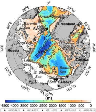
2 Data sets, model implementation, and methodology The Arctic Ocean is smaller in scale compared to other oceans: 7000 km at its widest point. The ocean is surrounded by a continental shelf with depths of 300 m. The center of the basin near the North Pole has depths greater than 4000 km and is often ice covered. The combination of ice coverage and geography creates the different regional seas shown in Fig. 1. We will distinguish seven sub-regions: (1) Nordic Greenland Sea, (2) Barents Sea, (3) Kara Sea, (4) Laptev Sea, (5) East Siberia Sea, (6) Beaufort–Chukchi seas, and (7) Baf-fin Bay. The following subsections describe the ice concen-trations, wind reanalysis, satellite altimetry, model setup, and analysis techniques.
2.1 Ice concentration from IFREMER/CERSAT (SSM/I)
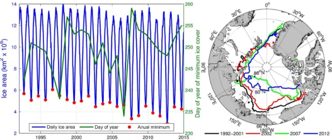
Satellite-derived ice concentrations are an invaluable data source to observe ice dynamics (e.g., Frey et al., 2015). The SSM/I brightness temperatures accurately estimate sea ice concentration (e.g., Liu and Cavalieri, 1998). The ASI al-gorithm of Kaleschke et al. (2001) uses a transfer equation that relates the polarization difference to ice concentration. High-frequency channels of SSM/I are used to estimate a daily average on a 12.5 km grid at IFREMER/CERSAT and describe important spatial features of the marginal ice zone (MIZ) (Ezraty et al., 2007). Figure 2 shows the minimum ice extent and total ice area for the period 1992–2014. The time series in the left panel confirms the continual decrease in ice
Figure 1. Regional seas of the Arctic Ocean with bathymetry (color), buoy locations (black symbols), and 4000, 2000, 500, and 100 m depth contours (black lines).
coverage. The minimum sea ice coverage is occurring later in September from 1992 to 2014 with some decadal vari-ability and/or anomalous years of 1997 and 2006. The sea ice is stable for 1992–2002. Following this period there is an accelerated reduction in sea ice extent with the ice min-imum occurring in 2012. The right panel shows the spatial view of the ice edge minimum from the years 1992 to 2002, 2002, 2007, and 2012. The East Siberia, Chukchi, and Beau-fort seas have the largest changes in ice cover so we expect increasing waves.
2.2 Reanalysis wind fields
Wave hindcasts using wind reanalysis data sets have success-ful applications including the National Center for Environ-mental Prediction (NCEP) Climate Forecast System reanaly-sis (CFSR) (Chawla et al., 2013; Rascle and Ardhuin, 2013; Stopa and Cheung, 2014). The important advancements of CFSR with respect to predecessors Reanalysis I and II con-sist of coupling between the ocean, atmosphere, land sur-face, and sea ice model, assimilation of satellite radiances, and increased horizontal and vertical resolution in the atmo-spheric model (Saha et al., 2010, 2014). The atmoatmo-spheric model has a resolution of approximately 0.3◦ (37 km) (v2
J. E. Stopa et al.: Waves in the Arctic 1607
Figure 2.SSM/I Ifremer CERSAT ice concentrations 1992–2014. The left panel displays the ice coverage in the area, assuming for grid points with a concentration greater than 15 % (blue) and minimum of the day of the year (green). The right panel shows the minimum spatial ice edge defined by the 15 % ice concentration contour for 1992–2001 (median), 2002, 2007, and 2012.
Wind speeds at 10 m elevation (U10) are available hourly. In addition, the wave reanalysis of the European Centre for Medium-range Weather Forecasts (ECMWF) ERA-Interim (ERAI), which couples the atmosphere and wave model and assimilates altimeter wave data, has improved performance over its predecessor ERA-40 (Dee et al., 2011). ERAI has a spatial resolution of 0.7◦with wind every 6 h. The wave
re-analysis couples the wave and atmosphere models while as-similating wave data from altimeters (Dee et al., 2011). The data set is consistent in time and does not have the same dis-continuous features as CFSR; however, it is not able to re-solve the upper percentiles (Stopa and Cheung, 2014).
It is not evident whether CFSR or ERAI is better suited to drive a wave model in the Arctic. Therefore a concurrent hindcast from 2010 to 2014 is used to assess the wind forcing differences on the wave field. Appendix A gives a detailed description of the results summarized here. The largest dif-ferences are in the upper percentiles and ERAI significantly underestimates the extreme wave heights. In short, the model errors mirror those of the global basin (Stopa and Cheung, 2014). Due to the importance of resolving the extremes, we use CFSR to re-create the waves from 1992 to 2014.
2.3 Significant wave heights from altimeters
Altimeter data have provided an ample source of global wave observations and aided in the development and eval-uation of spectral wave models (e.g., Chen et al., 2002; Ardhuin et al., 2010; Stopa et al., 2015). Significant wave heights (Hs) are measured from active microwave sensors
typically in the Ku or Ka bands under all atmospheric con-ditions. Once the data are quality controlled and sensor bi-ases are removed, Hs errors are comparable to buoy mea-surements (Zieger et al., 2009; Sepulveda et al., 2015). We use the merged and calibrated data set of Queffeulou and
Croize-Fillon (2016). The reprocessed wave measurements from European Remote Sensing satellites 1 and 2 (ERS1, ERS2), Environmental Satellite (ENVISAT), Geosat Follow-On, CRYOSAT2, and Altika SARAL are used throughout this study. The northern latitude limit is 81.4◦N for Geosat
Follow-On, 82◦N for ERS1, ERS2, ENVISAT, and SARAL,
and 88◦N for CRYOSAT2. The repeat track cycle is 17 days
for Geosat Follow-On, 35 days for ERS1, ERS2, ENVISAT, and SARAL, and 369 days for CRYOSAT2. The merged data set spans the duration of the hindcast (1992–2014).
2.4 WAVEWATCH III model implementation and wave–ice dissipation
WAVEWATCH III of Tolman et al. (2013) is a community-based spectral wave model (Tolman and the WAVEWATCH III Development Group, 2014). WW3 evolves the wave ac-tion equaac-tion in space and time, with discretized wave num-bers and directions. Conservative wave processes, repre-sented by the local rate of change and spatial and spectral transport terms are balanced by the nonconservative sources and sinks. We implement version 5.08 of WW3, on a curvi-linear grid matching the spatial resolution of ice concen-trations at 12.5 km. The curvilinear grid is well suited to model waves near the poles since the geographic distance be-tween nodes is equal making the computation more efficient (Rogers and Orzech, 2013). The spectra are composed of 24 directions and 32 frequencies exponentially spaced from 0.037 to 0.7 Hz at a relative increment of 1.1. The reanalysis winds are linearly interpolated to the wave model grid. We use WW3’s third-order Ultimate Quickest scheme by Tol-man (2002) with the garden sprinkler correction. Global 0.5◦
1608 J. E. Stopa et al.: Waves in the Arctic
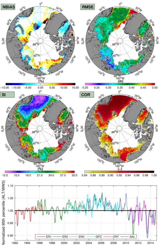
Figure 3.Top four panels display the normalized bias (NBIAS), root-mean-square error (RMSE), scatter index (SI), and correlation coeffi-cient (COR) for collocatedHsfor the CFSR wave hindcast and the merged altimeters 1992–2014. The bottom panel displays the normalized monthlyHs 95th percentile for each satellite platform: European Remote Sensing satellites 1 and 2 (ER1, ER2), Environmental Satellite ENVISAT (ENV), Geosat Follow-On (GFO), CRYOSAT2 (CRY), and Altika SARAL (SAL).
The source terms of Ardhuin et al. (2010) describes the wave physics, which performs well in terms ofHs, average
wave periods, and partitioned wave quantities (Stopa et al., 2015). The wind-wave growth parameterβmaxis set to 1.25
and otherwise we use the same settings as Rascle and
ve-J. E. Stopa et al.: Waves in the Arctic 1609
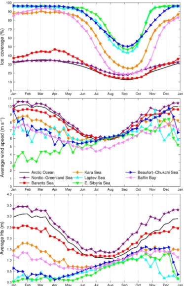
Figure 4.Ice coverage (top), wind speed (middle), andHs daily averages computed from a spatial average for each Arctic region showing the seasonality.
locity. This parameterization was calibrated using Wadhams and Doble (2009) data set but still remains somewhat poorly constrained. A full description of the formulation is given in Appendix B.
2.5 Wave parameters and analysis techniques
The wave climate is described using the total signifi-cant wave height (Hs) defined as Hs=4√m0 where m0
is the zeroth moment (p=0) of the spectrum (E(f ))
(mp=R0∞(2πf )pE(f )df), mean wave period (T m02= √
m0/m2), and average direction (θm). The mean wave
riod has reduced variability compared to other wave pe-riod definitions (i.e., peak pepe-riod or √m−1/m0) since it
is calculated from the second moment of the wave spec-trum. Swells characterized by longer wavelengths propagate considerable distances under sea ice while high-frequency waves are scattered and dissipated near the ice edge (Kohout
et al., 2014; Li et al., 2015; Ardhuin et al., 2015). There-fore the wind seas (Hsw,θmw) and swells (Hss,θms) are
ana-lyzed separately by partitioning wave spectra using the Han-son and Phillips (2001) method. According to PierHan-son and Moskowitz (1964) the sea state can be classified as wind sea when the wave age (WA) or ratio of peak phase speed
Cpto wind speed is WA=Cp/U10<1.2 and as swell when
WA>1.2. Semedo et al. (2011) and Semedo et al. (2014)
demonstrated the practicality of this classification through the probability of having a swell-dominated wave field (swell persistence):Ps=P (Cp/U10>1.2)=Ns/Ntotal, whereNs is the number of swell-dominated events andNtotalis the total number of events.
In seas with varying ice cover, the method to describe wave statistics is important (Tuomi et al., 2011). We base our statistics on ice-free conditions (ice concentration<15 %),
but other statistics can be interrelated through the sea ice probability shown in Appendix C. Our results are calculated using the 3 h model output for the hindcast duration.Hs
per-centiles are calculated from the ice-free statistics and the matchingHs index is used to identify corresponding wave periods and directions. A±0.2 m bounds of the associated
Hsindex is used to average the wave periods and directions. This approach gives a more accurate physical description of the events (Anderson et al., 2015). We compute trends us-ing Sen’s method and test for statistical significance with the Mann–Kendall test. This method is a non-parametric technique and a robust way of computing trends since it can handle missing data and is less influenced by outliers (Mann, 1945; Kendall, 1975; Sen, 1968). We account for the seasons using the adaptation of Hirsch et al. (1982) and used in wave climatology studies by Wang and Swail (2001), Young et al. (2011), and Stopa and Cheung (2014). We com-pute trends from monthly statistics and require that the time series be ice free for at least 10 years.
3 Wave hindcast validation
Before the wave climate is assessed we validate the hind-cast using the merged altimeter data set for 1992–2014. Altimeter–model co-locations are found using the nearest neighbor within 6 km and 30 min. A running mean of 5 points smooths the satellite tracks to make the spatial and tempo-ral scales comparable. The top 4 panels of Fig. 3 show four complementaryHs statistics computed in 25 km bins. There
1610 J. E. Stopa et al.: Waves in the Arctic
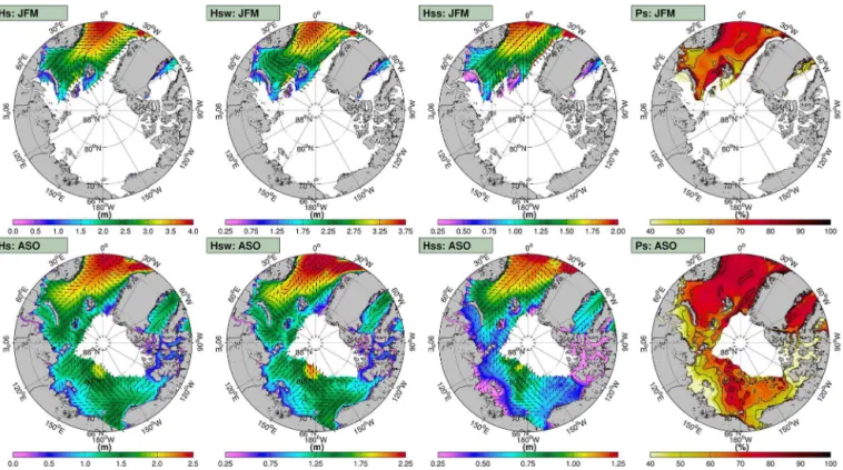
Figure 5.January–February–March (JFM) and August–September–October (ASO) seasonal averages ofHs(first column), wind-sea wave heightHsw(second column), swell wave heightHss(third column), and swell persistencePs(fourth column). The directions are computed from by averaging the east–west and north–south components separately.
and the SSM/I daily input might not be able to resolve the rapid change. The Nordic Greenland Sea is mostly ice free year round and thus has the lowest scatter indices (12 %), suggesting the model performs well in the absence of sea ice, in contrast to the coastal regions of the Baffin Bay, Kara, Laptev, and Beaufort seas that have considerable ice variabil-ity and create the largest scatter indices of 30 %. The model and altimeters are highly correlated with coefficients larger than 0.95. The lowest correlations occur in the Laptev, East Siberia, and East Beaufort seas. These regions have small wave heights and result in small biases and RMSEs.
The bottom panel of Fig. 3 shows the consistency of hind-cast using the monthly 95th percentile for each satellite mis-sion. The 95th percentile is a rigorous test because it is dif-ficult to resolve extreme waves. The average and median are verified to have no distinct trends (not shown). There is a slight decreasing trend in recent years but it is inconclusive whether this trend will continue and is contrary to the global increase observed by Rascle and Ardhuin (2013) for 2006– 2011. There are annual variations but the hindcast is rela-tively consistent in time, making it applicable for climate studies with no noticeable discontinuous features.
4 Wave climate
4.1 Seasonality
J. E. Stopa et al.: Waves in the Arctic 1611
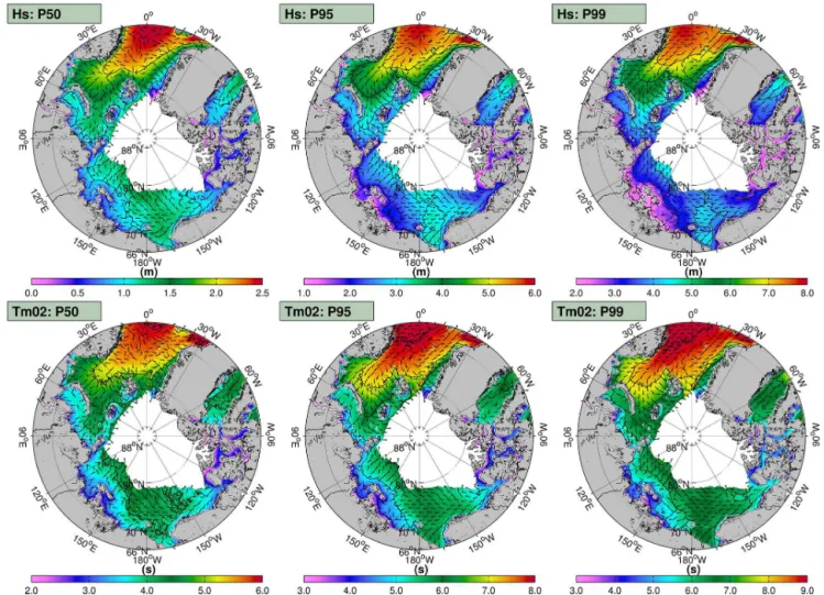
Figure 6.Significant wave height percentiles (top panels) and corresponding averaged wave periods (bottom panels) and directions (arrows).
Figure 5 presents the wave conditions for the two extreme seasons: JFM and ASO. The sea state is described through the Hs,Hsw,Hss, andPs. In JFM, only the Nordic Green-land, and Barents seas are ice free. Waves generated in the North Atlantic propagate into these seas with a sheltering in the Barents Sea. In JFM, the Nordic Greenland Sea has the tallest wave heights of the Arctic. The wind seas follow the driving winds and are characterized by cyclonic (anti-clockwise) circulation, a characteristic of the North Atlantic sub-basin (Sterl and Caires, 2005; Semedo et al., 2014). The resulting wind-sea wave heights exceed 3.5 m while the swell wave heights are smaller and travel from the southwest. The top right panel shows swells persist 70 % of the time, which is consistent with open ocean conditions where wind seas and swells are ubiquitous (Chen et al., 2002).
In ASO, ice coverage is minimum and waves are gener-ated across the Arctic. TheHspattern in the Nordic, Green-land, and Barents seas is similar to JFM with only a reduc-tion in magnitude. The semi-enclosed seas have smallerHs
(commonly less than 1.5 m) than the Nordic Greenland Sea. There are distinct regional characteristics of the wind seas
and swells. The cyclonic structure of the wind seas near Nor-way in JFM is not clearly visible in ASO. The swell mean wave directions follow the same pattern as JFM in the Nordic Greenland and Barents seas and propagate from the Atlantic northward into the sea ice. In the Laptev and East Siberia seas the wind seas and swells are directed into the sea ice with an Easterly component.HswandHsshave local
max-ima located near (170◦E, 77◦N) where the easterly waves
are able to sufficiently develop. In the Beaufort Sea the wind sea and swell mean wave directions flow from the southeast. In the East Beaufort Sea (135◦E, 74◦N), there is a subtle
anti-cyclonic (clockwise) structure in the wind seas while the swell mean wave directions are opposite and flow from the west. In the narrow corridor of the Baffin Bay, the wind sea and swell mean wave directions are opposite and represent different phases of passing storms. The bottom right panel shows the swell persistence is>85 % and exceeds 95 % in
1612 J. E. Stopa et al.: Waves in the Arctic
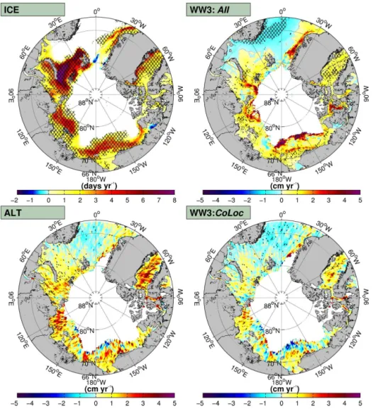
Figure 7.Ice coverage andHstrends given by Sen’s slope with the Mann–Kendall test (thatched areas). The top left panel displays the trend of the annual number of ice-free days per year (ICE). The other panels show the trends of monthly averagedHsdata sets: using the entire 3 h hindcast (top right: All), altimeters (bottom left: ALT), and co-located hindcast (bottom right: CoLoc) given in cm year−1.
Beaufort, and Chukchi there is an equal proportion of wind waves and swells (40–60 %).
4.2 Percentiles
Hs percentiles are a useful to way to describe the sea state statistical distribution (e.g., Stopa et al., 2013a, b). Figure 6 shows the 50th (median), 95th, and 99thHspercentiles with matching wave directions and mean periods. The statistics have a consistent spatial pattern due to the geographic shape of the basin. The most prominent feature is the maximum located in the Nordic Greenland Sea for all percentiles. Here the medianHsexceeds 2.5 m and correspondingT m02 is 6 s.
In the rest of the basin the Hs median is commonly 1.5 m with reduction near the coasts. The 95th Hs percentile ex-ceeds 5.5 m withT m02 of 8 s in the Nordic Greenland Sea.
In the Laptev, East Siberia, Chukchi, and Beaufort seas the 95thHspercentiles are 2.5 m withT m02 of 6 s. TheHsand
T m02 at the 99th percentile exceed 8 m and 9 s in the Nordic
Greenland Sea while in the Laptev, East Siberia, Chukchi, and Beaufort seas are reduced with 4 m and 6.5 s.
J. E. Stopa et al.: Waves in the Arctic 1613
Figure 8.Sen’s slope with the Mann–Kendall test (thatched areas) for monthly averaged wind speeds (U10) (top left), wind-sea wave heights (Hsw) (top center), swell wave heights (Hss) (top right), average wave period (T m02) (bottom left), wind-sea steepness (STw) (bottom center), and wave age (WA) (bottom right) from the wave hindcast in percentage per year relative to the average.
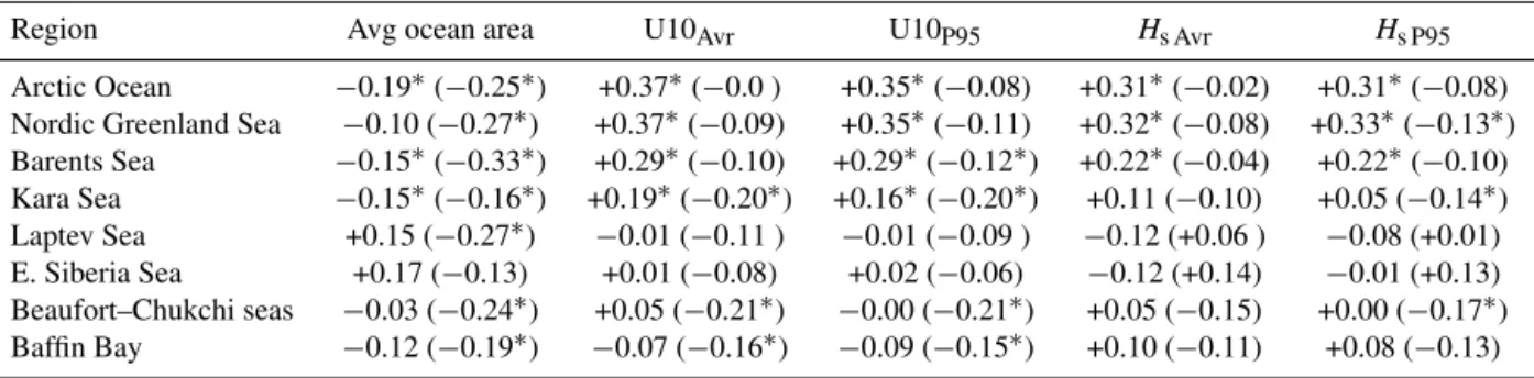
Table 1.Correlation coefficients and trends for the various regions and parameters. The correlations coefficients are given between area-averaged monthly time series versus the North Atlantic Oscillation and the Pacific Decadal Oscillation in parentheses. Statistically significant results are given by the * when thepvalue is less than 0.05.
Region Avg ocean area U10Avr U10P95 Hs Avr Hs P95
1614 J. E. Stopa et al.: Waves in the Arctic
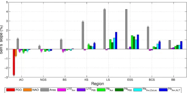
Figure 9.Sen’s slope with the Mann–Kendall test (denoted by a *) for the Arctic regions of the Arctic Ocean (AO), Nordic Greenland Sea (NGS), Barents Sea (BS), Kara Sea (KS), Laptev Sea (LS), East Siberia Sea (ESS), Beaufort–Chukchi seas (BCS), and the Baffin Bay (BB) from monthly time series of the North Atlantic oscillation (NAO), Pacific Decadal Oscillation (PDO), ocean area (Area), wind speed (U10), significant wave heights from the 3 h model data (Hs AvrandHs P95), and co-located model and altimeter data (Hs Avr,CoLoc,Hs Avr,ALT).
Beaufort, Chukchi, and East Siberia seas, the waves from the east are common to both the wind waves and swells in JFM and ASO.
4.3 Trends
With the reduction of sea ice cover, wave heights are ex-pected to increase. Figure 7 shows Sen’s slope computed from monthly averaged quantities with the seasonal Mann– Kendall test for ice coverage andHsfrom altimeters and the
model. The top left panel displays the trend of the SSM/I ice concentrations in number of days per year that are ice free (i.e., concentration <15 %). Most of the ice-covered areas
are statistically significant and are ice free on 2 additional days each year. The strongest trends are located in the Bar-ents and Kara seas with 8 more ice-free days per year. The isolated regions near Svalbard, Greenland, and the Amund-sen Gulf have increasing ice coverage.
Most of the basin has increasing wave heights shown by the altimeters and wave model in the top right and bottom panels. The bottom panels show that the co-locatedHstrends from the altimeters and the model agree, despite the stronger trends in the altimeters. However, the altimeter confidence interval encompasses the model results so statistically they are equivalent. This is a verification that the CFSR forc-ing is homogeneous throughout this time period. Discrete satellite passes do not capture the complete space–time his-tory, causing spurious trends especially near the MIZ in the East Siberia and Beaufort seas. The trends computed from the continuous hindcast in the top right panel show a spa-tially consistent pattern. The ice variability is expected to cause the discrepancies in the East Siberia and Beaufort–
Chukchi seas that exist comparing the top and bottom pan-els. The Nordic Greenland Sea is the only region with a con-sistent statistically significant decreasing trend shown in the top right panel. In the Beaufort–Chukchi seas, our rates of 1.5 cm year−1 are in agreement with Francis et al. (2011),
who estimated a trend of 2 cm year−1. Wang et al. (2015)
es-timated trends on the order of 40 cm computed by the differ-ence between 1970–1991 and 1992–2013. Assuming a linear rate spanning the 23-year period, our rate equates to a 35 cm increase. Some extreme trends greater than 4 cm year−1
exist in the Baffin Bay and Laptev Sea and are statistically significant using the merged altimeters. These rates are large compared to the global calculations of Young et al. (2011), who estimated the largest trends to be 2 cm year−1.
Figure 8 shows the Sen’s slope computed from other monthly averaged parameters. The rates are presented as per-centages relative to the mean to allow comparison. The trends in U10 are calculated using the entire data set independent of ice cover; otherwise all other variables are computed from ice-free statistics. The decreasing U10 trend in the Nordic Greenland Sea is significant and is consistent with theHs trend. Across most of the sea ice, U10 is decreasing espe-cially in the Beaufort Sea. Some regions have weak increas-ing trends of 0.25 % per year. Wind speeds in the Baffin Bay are increasing creating taller wave heights.
The T m02 trends follow the same pattern as the wave
heights in Fig. 7 and with an increase of 2 % (2–3 cs) per year. The Hsw andHss trends have similar spatial patterns
asHs. However,Hss is increasing at a faster rate compared
J. E. Stopa et al.: Waves in the Arctic 1615
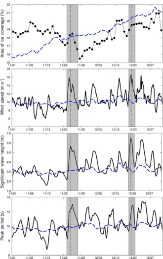
Figure 10. Area-averaged ice coverage, wind speed, significant wave height, and peak period in the Greenland Sea for November– December 1992 (solid line). The dashed line is the daily average from 1992 to 2014.
Nordic Sea has less statistically significant points, suggest-ing changes in the local winds are caussuggest-ing the trends. The bottom-center panel displays the wind-sea steepness (STw) (ratio of wind-sea wave height versus wavelength). The wave steepness reduces, illustrating that the wavelengths become longer than the wave heights are becoming taller. However, the trends in swell steepness have the same pattern as Hs,
meaning the swell wavelengths are changing proportionally to the heights (not shown). Finally, the WA is increasing across the entire domain, albeit some decreasing regions exist near the MIZ in the Beaufort Sea, Greenland Sea, and Baf-fin Bay. Consequently the wave phase speeds are increasing faster than the driving wind fields and swells are becoming more prevalent.
Trends often contain a component of natural variability which may lead to opposite trends in the future. The North Atlantic Oscillation (NAO) has a strong influence in the Nordic Greenland Sea shown by Semedo et al. (2014) and in the Beaufort–Chukchi seas, the Pacific Decadal Oscilla-tion (PDO) influences the ice and wind dynamics (Frey et al.,
2015). Table 1 presents correlation coefficients between area-averaged monthly time series of sea ice, U10, andHsand the
NAO and PDO indices (see Appendix D for spatial distribu-tion). The statistically significant relationship in the wind and wave fields with the NAO is moderate in the Nordic Green-land and Barents seas. In these seas, a positive NAO phase equates to increased sea states while negative phases have re-duced sea states. The NAO was positive in the beginning of the time period (1992–1998) and negative towards the end of the hindcast (2006–2012). This creates a negative trend and its positive relationship with the sea states and wind suggests the NAO is causing the negative wind and wave trends ob-served in Nordic Greenland and Barents seas. Table 1 shows that the PDO is weakly related in the Beaufort–Chukchi seas. Higher values are attained by correlating the time series for each point (see Appendix D).
Figure 9 summarizes the regional trends through Sen’s slope of the NAO, PDO, ice-free area, U10, and Hs.
The NAO and PDO have statistically significant decreasing trends. The NAO is influencing the decreasing trend in the Nordic, Greenland, and Barents seas seen in Figs. 7 and 8. The most prominent feature is the increase in ocean area or reduction of ice cover. TheHs trends are not homogeneous showing the regional variability. The largest trends in ocean-area andHs occur in the Laptev and East Siberia seas. All seas except the Baffin Bay have stronger trends in the aver-ageHs compared to the 95th percentile, suggesting nonuni-form changes in the statistical distributions. When the av-erage trend is higher than the 95th percentile it means that moderate events occur more frequently compared to an inten-sification of strong events. In the Baffin Bay the trends in the 95th percentile are larger than the average, suggesting the in-tensification of strong events. The wave trends computed for the co-located altimeters and model show the model underes-timates (consistent with Fig. 7). TheHsaverage and 95th
per-centile have larger trends than the results in the global ocean, which were typically less than 1 % (Young et al., 2011). The trivial U10 trends illustrate that the increased sea states are due to the reduction of ice cover in agreement with Wang et al. (2015).
5 Wave impact on the sea ice
1616 J. E. Stopa et al.: Waves in the Arctic
Figure 11.Wind speeds, significant wave heights, and peak periods for events in November and December 1992. The arrows denote the wind direction or average wave direction. The contour lines represent the 15 % ice concentration before (white) and after (black) the event.
environments are different: the Nordic Greenland seas are in-fluenced by swells from the North Atlantic and the Beaufort– Chukchi seas is characterized by an equal mix of wind waves and swells coupled with an extreme change in seasonal ice coverage.
Figure 10 shows the Nordic Greenland Sea area-averaged ice and sea state conditions for 2 months in 1992. The 23-year climate average (dashed line) shows the ice cover clima-tology increases 6 % from November through December. The first event, on 23–29 November, indicates a decrease in ice cover by−3 % or∼60 000 km2. This event coincides with
Hs, peak periods, and wind speeds exceeding 5 m, 12 s, and
14 m s−1, respectively. The second event in December has larger wave heights (>6 m), but the ice cover remains the
same.
We compare and contrast these two events in Fig. 11 by showing snapshots of the wind speed, wave height, and wave period. During the November event, the ice edge changes considerably before and after the event (white and black lines). The wind field rotation is cyclonic and centered near Iceland (14◦W, 66◦N). An anti-cyclonic pattern (6◦E,
78◦N) adds to the effective fetch. U10 exceeds 20 m s−1and
Hs exceeds 9 m close proximity to the ice with wave
peri-ods ranging from 12 to 15 s. Further into the sea ice only the largest wave periods remain due to the attenuation of the short wavelengths. The wind and wave directions are largely perpendicular to the Greenland ice edge. The largest sea ice changes are located from 70 to 77◦N, corresponding to the
maximum wave energy and wind speed. The bottom panels of Fig. 11 show the December storm is located further (7◦E,
71◦N) from the Greenland ice edge. This leads to a reduction
of wind speeds (<18 m s−1), wave heights (3 m), and periods
(12 s) close proximity to the ice edge. The minimal change in ice coverage is related to the reduced wind and wave energy entering the ice. We do not consider the ice thickness in our analysis; therefore it is not apparent how much ice volume is lost by either event.
Figure 12 shows the ice cover and sea state conditions in the Beaufort–Chukchi seas in September and October 2006. During this time of year the ice increases and advances southward. Both 13–16 September and 9–11 October have changes in sea ice coverage. In the first event the ice coverage reduces by 12 %, equating to 226 000 km2, while in the sec-ond event the decrease of 6 % equates to 113 000 km2. The second event hasHs of 6 m, which is well above the clima-tology average of 2 m. The sea state is much weaker in the first event than in the second.
Figure 13 illustrates the corresponding sea state condi-tions. The September case has winds predominately from the South directed into sea ice from the Bering Strait. The wind speeds are strengthened by the pressure gradient force cre-ated by the tall mountain ranges in Alaska and Russia which exceed 2 km in height. The wind speeds, wave heights, and periods reach 18 m s−1, 4.5 m, and 9 s offshore of the ice. The area of polynya located near (158◦W, 77◦N) does not
J. E. Stopa et al.: Waves in the Arctic 1617
Figure 12. Area-averaged ice coverage, wind speed, significant wave height, and peak period in the Beaufort–Chukchi seas for September–October 2006 (solid line). The dashed line is the daily average from 1992 to 2014.
significant changes to the ice edge and a large indentation coincides with the maximum wind and wave energy. Besides this isolated section, the rest of the Beaufort ice edge re-mains the same. The October event has large wind speeds, wave heights, and wave periods exceeding 24 m s−1, 8 m, and
13 s. In fact, this is the strongest event from 23-year hindcast andHs. The wave heights exceed 8 m and are well above the 99th percentile of Fig. 6. The wind field has a cyclonic pat-tern confirmed to be a polar low centered in the Chukchi Sea (162◦W, 62◦N) and an anti-cyclonic pattern (high-pressure
system) centered over the sea ice (132◦W, 80◦N). The
po-sitions of these systems create an extended fetch for wave development because the eastern winds are directed paral-lel to the sea ice. Ekman transport could be moving warmer water towards the sea ice. In addition, the extreme wind and waves enhance mixing, which could transport warm waters to the ice. As time evolves the systems move further north
creating a larger southerly component in the eastern portion of the domain where significant impacts occur in the sea ice coverage.
These examples suggest a relationship between the evo-lution of sea ice and the amount of wind and wave energy directed into the MIZ. The incident angle of the winds and waves to the sea ice plays a critical role on sea ice, so the location of the storm relative to the ice edge is important. Other physical processes that influence sea ice include tem-perature change, ocean circulation, and transport due to wind (Frey et al., 2015). These examples illustrate how waves im-pact the sea ice and should be considered as a potential sea ice driver.
6 Discussion
Coupling between waves and sea ice is complex (e.g., Squire et al., 1995; Squire, 2007). While the inclusion of the wave– ice dissipation term is a step to incorporate improved wave– ice processes within the wave model, redistribution of the wave energy through scattering must also be considered (Squire et al., 1995). Furthermore, wind-wave generation in partially ice-covered waters is expected to be more com-plex than as parameterized in present wave models (Li et al., 2015). Despite these missing physical processes, the 23-year hindcast presented here performs well offshore of the sea ice as demonstrated by theHscomparison to the altimeters.
The wave conditions in the Arctic are governed by the sea ice and winds and we observe two distinct regions: (1) semi-enclosed basins and (2) region exposed to the North At-lantic. The semi-enclosed and isolated seas of Kara, Laptev, East Siberia, Beaufort–Chukchi, and Baffin Bay makes them event driven and explains why they have an equal mix of wind seas and swells. Here the sea state magnitudes are com-parable to those in the Gulf of Mexico (Stopa et al., 2013a). The Atlantic side of basin has the most active sea states be-cause it is exposed to the Atlantic and is mostly ice-free year round. Here the wave seasons follow the winds and behave like a sinusoid. Extreme events in these seas are limited by the basin’s size and the wave directions are parallel to the ice edge. Therefore, to a leading order the wave behavior is linked to the geography and ice conditions which control the effective fetch for wave development (Thomson and Rogers, 2014; Smith and Thomson, 2016).
1618 J. E. Stopa et al.: Waves in the Arctic
Figure 13.Wind speeds, significant wave heights, and peak periods for events in September and October 2006. The arrows denote the wind direction or average wave direction. The contour lines represent the 15 % ice concentration before (white) and after (black) the event.
with prior studies (Wang et al., 2015; Francis et al., 2011). If these trends continue the sea state will continue to increase as well. The Arctic sea ice in the semi-enclosed basins are more sensitive to the wave conditions in the fall compared to the other seasons due to concurrent increasing winds and partially open seas this time of year. Therefore we expect the Arctic to be very sensitive to changes in sea ice, winds, and waves in the fall compared to any other time period. This has led Thomson and Rogers (2014) and Thomson et al. (2016) to suggest a positive feedback mechanism linking enhanced wave heights to the larger ocean expanses which cause more ice breakup. However, this process is convoluted by the fact that the wave steepness is lessened, which reduces the effec-tiveness of the ice breakup by waves.
The wave response to the changing sea ice through the 21st century is complex, with a mix of influences from wind, sea ice, and climate variability (Khon et al., 2014). In the major-ity of the Arctic, wave heights are increasing. The only region with decreasing wave heights is in the Nordic Greenland Sea. In our hindcast time period of 1992–2014, the natural vari-ability of the climate through the NAO and PDO impacts the Arctic sea state. The negative trends observed in the sea state are expected to be caused by the NAO. The PDO influences the Barents and Kara seas and the monthly correlation co-efficients closely aligns with the maximum ice loss. In the Beaufort–Chukchi seas the PDO plays a minor role in the wind and wave fields, but this should be monitored when the PDO transitions into a positive phase.
J. E. Stopa et al.: Waves in the Arctic 1619 7 Conclusions
Extending previous studies of Francis et al. (2011), Wang et al. (2015), and Semedo et al. (2014) to the Arctic, we produced a 23-year wave hindcast from 1992 through 2014 using CFSR winds and ice concentrations from SSM/I. The combined use of models and satellite observations proves to be a robust way of monitoring and describing the climate. As the Arctic continues to change, the results presented here can be used as a basis for future climate studies or projections such as those presented by Khon et al. (2014) or Dobrynin et al. (2012). Our observed changes in the wave field are ex-pected to be influencing the coastlines, ecosystem, and sea ice melt (e.g., Overeem et al., 2011; Tremblay et al., 2008; Popova et al., 2010; Davis et al., 2016). Since the Arctic is semi-enclosed, the sea states are event driven and this cre-ates distinct features in the wind seas and swells. If the open ocean persists later into the fall, then the sensitivity of the Arctic sea state and ice conditions will increase since this season has stronger wind speeds. The reduction in ice extent enhanced sea states with taller wave heights, longer wave-lengths, and more persistent swells. While it is not evident how important wave–ice processes are within the Earth sys-tem, the increasing sea states in the Arctic do have critical and direct implications on the environment.
8 Data availability
1620 J. E. Stopa et al.: Waves in the Arctic Appendix A: The ECMWF-Interim reanalysis and the
NCEP Climate Forecast System Reanalysis arctic intercomparison 2010–2014
Before the 23-year hindcast was implemented, we intercom-pared two 5-year hindcasts using CFSR and ERAI winds to establish the better-suited wave forcing. Measured wave data are essential for validation and we use buoy and altime-ter observations. Only a limited number of buoys are avail-able from the National Data Buoy Network (NDBC) in the Chukchi Sea and their locations are shown in Fig. 1. Only select years and Hs measurements are available from July through October (2012–2014) in depths less than 50 m. Stan-dard error metrics are used to assess the models including the normalized bias (NBIAS), RMSE, correlation coefficient (R), scatter index (SI), and normalized standard deviation
(NSTD), wherexrepresents the observation,yrepresents the
model, andnis the number of data pairs:
NBIAS= "
(y−x) / 1 n
n X
i=1
xi2
!#
×100 (A1)
RMSE= v u u t 1 n n X
i=1
(yi−xi)2 (A2)
R=
n X
i=1
(yi−y) (xi−x) / v u u t 1 n n X
i=1
(yi−y)2
v u u t 1 n n X
i=1
(xi−x)2 (A3) SI= v u u t 1 n n X
i=1
(yi−y)−(xi−x)2/x
×100 (A4)
NSTD= v u u t 1 n n X
i=1
(yi−y)/ v u u t 1 n n X
i=1
(xi−x)/−1
×100. (A5)
Table A1 displays errorHsmetric with the NDBC buoys. The CFSR hindcast overestimates theHs by at least 5 % at all locations while the ERAI hindcast underestimates by 3 % (except WMO48213). The RMSEs are commonly 0.25 m, with the ERAI hindcast always having a better agreement. The scatter indices and correlation coefficients for the ERAI and CFSR wave hindcasts are similar at each buoy. The NSTD shows the CFSR hindcast has more variability than the observations while the ERAI hindcast is smoother. In general both hindcasts are comparable but the CFSR hind-cast has a positive bias while the ERAI hindhind-cast has a nega-tive bias.
Figure A1 displays two example time series from Septem-ber 2013 and 2014 at buoys WMO 48213 and 48214 located in the Chukchi Sea. The first example in 2013 shows both models perform reasonably well. The time series of the ERAI hindcast is smoother and has a correlation coefficient of 0.89. The CFSR hindcast is seen to overestimate the events on 1– 3 and 26–28 September with differences larger than 0.5 m. For these events the ERAI hindcast follows the same pat-tern, suggesting a systematic error in the forcing wind field or wave physics that are unresolved. The hindcast residu-als (CFSR-buoy and ERAI-buoy hindcasts) are moderately correlated with coefficients of 0.75, showing that the forcing wind fields are similar. In September 2014, both ERAI and CFSR hindcasts are highly correlated to the buoy time series and their residuals are only weakly correlated with a coeffi-cient of 0.37. The CFSR hindcast has a consistent positive bias throughout the month, while the ERAI hindcast com-monly has errors less than 25 cm. Notice that the peak inten-sity of wave events is underestimated by the ERAI hindcast. Figure A2 summarizes theHscomparison from the
altime-ter and model co-locations using the 5-year period. The scat-ter plots from all 2 million data pairs is presented in the top panels. Both data sets are highly correlated with similar SIs of 19 % and have RMSEs of∼0.4 m. The smooth nature of the ERAI hindcast creates the negative NSTD of 10 % while the CFSR hindcast is nearly 0. The largest differences be-tween the hindcasts are in the upper wave heights and the bottom panels highlight the differences. Both data sets have similar correlation coefficients of 0.78 and scatter indices of 13 %. The CFSR hindcast has more variability than the ob-served data, creating a NSTD of 20 % while the ERAI hind-cast matches the variability of the observations much bet-ter. From this depiction it is clear that the ERAI hindcast underestimates the largest wave heights. For example, the 99thHs percentile has an average bias of −1.5 m while it
is−0.1 m for the CFSR hindcast. These large sea states are important to resolve in practical planning and engineering applications. Therefore caution should be applied when us-ing extreme waves from a hindcast that uses ERAI winds as forcing. In our implementation of the ERAI hindcast,βmax described in Ardhuin et al. (2010) is set to 1.45 and possibly a better match could be achieved by increasing this value.
J. E. Stopa et al.: Waves in the Arctic 1621
Table A1.Hserror metrics for select years in the Beaufort–Chukchi seas using CFSR and ERAI in parentheses.
Buoy ID Depth (m) Years valid (YY) N NBIAS (%) RMSE (m) SI (%) R NSTD (%)
All – 12,13,14 7574 +8.44 (−3.14) 0.29 (0.25) 20.71 (20.05) 0.94 (0.94) +1.42 (−5.55) WMO48213 50.01 13 1700 +11.40 (+1.36) 0.31 (0.28) 25.99 (26.39) 0.91 (0.91) +6.22 (+6.97) WMO48214 36.13 12,13,14 3956 +7.79 (−3.52) 0.27 (0.24) 17.55 (16.43) 0.94 (0.95) +0.79 (−9.06) WMO48213 41.16 12 568 +5.66 (−3.67) 0.28 (0.23) 15.68 (13.57) 0.95 (0.95) −11.66 (−10.30) WMO48211 32.52 13 1350 +9.95 (−8.22) 0.30 (0.26) 30.72 (27.53) 0.87 (0.88) +10.61 (−13.24)
1622 J. E. Stopa et al.: Waves in the Arctic
Figure A2.Significant wave height comparison from CFSR (left) and ERAI (right) versus co-located data from altimeters. The error dis-persion of the models is presented in a scatter plot with the density given in a logarithmic scale (top panels). The upper percentiles are highlighted to show the differences (bottom panels).
statistical distributions at the 99.9 % confidence limit for the entire domain. Figure A4 shows the probability distributions of the hindcasts, buoys, and altimeters. The CFSR hindcast matches the wave heights larger than 2.5 m well, while the ERAI hindcast consistently underestimates. When theHs is less than 2.5 m the CFSR hindcast overestimates. The ERAI hindcast tends to favor the small wave heights. The buoy comparison in the right panel shows similar features. Here the CFSR hindcast overestimates average wave heights of 1– 2.5 m, which agrees with the examples shown in Fig. A1. Therefore we can conclude that the extreme waves and the average conditions are different in the two hindcasts.
In conclusion, both data sets perform reasonably well and their results agree with errors found in the global ocean (Stopa and Cheung, 2014). The CFSR wave hindcast con-sistently predicts higher wave heights for average sea states and matches the upper percentiles much better. The upper wave heights in the ERAI hindcast diverge from the observa-tions and the 99th percentile has an average bias of 1.5 m. In
J. E. Stopa et al.: Waves in the Arctic 1623
Figure A3.The 50th and 99thHs CFSR percentiles (2010–2014) (top left and middle panels). ERAI–CFSR 50th and 99th percentiles are given in the bottom left and middle panels. The top right panel shows the correlation coefficients between ERAI and CFSR for a monthly averaged time series between CFSR and ERAI. The Mann–Whitney test is presented in the bottom right panel at the 99.9 % confidence limit.
1624 J. E. Stopa et al.: Waves in the Arctic Appendix B: Theoretical formulation of friction under
ice plates
B1 Extension of the theory by Liu et al.
The representation of dissipative source terms in spectral wave models can generally be cast in a quasi-linear form (Komen et al., 1994):
S(f, θ )=βσ E(f, θ ), (B1)
whereE(f, θ )is the frequency-direction spectrum of the
sur-face elevation,σ=2πf, andβis a nondimensional
dissipa-tion coefficient that is negative when wave energy is actually dissipated. Previous treatments of the dissipation of wave en-ergy due to friction below an ice layer have been confined to a laminar viscous boundary layer and presented by (Liu and Mollo-Christensen, 1988):
βv= −k p
νσ/2/(1+kM), (B2)
in whichkandσ are the wave number and radian frequency,
related by a dispersion relation that can be affected by the ice, andMis the ice inertia effect related to the ice thickness
multiplied by the ratio of ice to water density. In the present paper, because we focus on the dominant long-period waves for which the effect of the ice is less, we have used the ice-free dispersion relationσ2=gktanh(kD)in whichDis the
water depth andgthe acceleration of gravity. For these long
waves, the factorkMin Eq. (B2) can be neglected.
For practical applications, the obtained dissipation coeffi-cientβwas then scaled up to fit observed wave attenuations
by replacing the molecular viscosity at the freezing tempera-ture of sea water,ν≃1.83×10⁻⁶m2s−1, by an eddy
viscos-ity that was proposed to be as large as 0.3 m2s−1(Liu et al., 1991). Such a change in viscosity only makes sense when the flow is turbulent. Further, the functional form of the dissipa-tion can be very different for laminar and turbulent fricdissipa-tions in an oscillatory flow near a boundary, as observed by (Jensen et al., 1989). In turbulent boundary layers, the energy dissi-pation coefficient typically grow with the wave amplitude, leading to a dependence ofβ on the wave amplitude.
We thus revisit this question and propose a parameteri-zation for the laminar to turbulent transition of the bound-ary layer below the ice. In turbulent conditions, an impor-tant parameter is the roughness length below the ice z0. That roughness is unfortunately not well known, with only a few measurements of current boundary layers (e.g., McPhee and Smith, 1976). Because the roughness for the wave mo-tion is probably different from the roughness for the cur-rents, as it is well known for ocean bottom boundary layers (Grant and Madsen, 1979), we are left with the difficulty of defining the value ofz0. Given this roughness, the orbital
ve-locity profile is expected to follow a Kelvin function (Grant and Madsen, 1979) with a dissipation source term that takes a form similar to that of bottom friction (e.g., Madsen et al.,
5 6 7 8 9 10 11 12 13 14 151617181920 104
105 106
Wave period (s)
Half − decay distance Viscous Turbulent Combined rayleigh Combined smooth
Figure B1.Half-decay distances as a function of the wave period T and the significant wave heightHs.Hsis varied from 0.5 (upper curves) to 5 m (lower curves). The combination of viscous and tur-bulent expressions is made using either a Rayleigh distribution of wave height and computing the dissipation for each wave height in the distribution or by a smooth linear combination of the viscous and turbulent terms adjusted to reproduce the Rayleigh result.
1990; Ardhuin et al., 2003) or swell dissipation by friction at the air–sea interface:
βt= −feuorb/g, (B3)
where the significant orbital amplitudes of the surface veloc-ity is, for deep water waves,
uorb=2 v u u u t ∞ Z 0
(2πf )2E(f )df . (B4)
fe is the same dissipation factor used for bottom friction,
which is a function only of the ratioaorb/z0, where aorb is the significant orbital displacement at the sea surface, here for deep water wavesaorb=Hs/2.
From bottom and air–sea boundary layer studies, the tran-sition from laminar to turbulent is expected to occur at a thresholdRecof the significant Reynolds number defined by
Re=uorbuorb/ν. (B5)
We take the same critical valueRec=1.5×10⁵found for the
J. E. Stopa et al.: Waves in the Arctic 1625 Rayleigh distribution is well approximated by the following
combined dissipation parameter
βc=(1−w)cvβv+wctβt, (B6)
in whichcv andct are empirical adjustment constants,
ex-pected to be close to 1, and the weightwtransitions smoothly
with the value ofReover a range1Re=200 000:
w=0.51+tanh((Re−Rec)/1Re). (B7)
Figure B shows the expected decay distance as a function of frequency, due to molecular viscosity (blue) or a turbulent boundary layer with a roughnessz0=0.1 mm, for significant
wave heights ranging from 0.5 to 5 m. In our applications we have chosenz0=1 cm.
B2 Empirical adjustment of the wave attenuation (Wadhams and Doble, 2009) have reported measurements of waves with periods larger than 20 s far into the ice pack (the periods reported in the paper were erroneously reduced by a factor 1.5; personal communication of M. Doble, 2015). An event with 20 s waves recorded 1400 km into the ice pack on 13 February 2007 had a maximum significant wave height of 3 cm. For this small wave height the wave boundary layer is expected to be laminar. However, using the dissipation coeffi-cient in Eq. (B6) produced maximum wave heights of 30 cm. Changing only the coefficientcv, it was necessary to increase
it from 1 to 8 to obtain a reasonable agreement with the data. We have thus used that value to obtain reasonably small wave heights across the Arctic.
However, we note that cv=8 tends to overestimate the
dissipation in the Southern Ocean case discussed by (Ard-huin et al., 2015), for which cv≃2 is a better adjustment.
Such differences could be partly caused by a more complex geometry of older ice in the Arctic, but a 4-fold increase of the area of the ice–water interface that could explain this difference is unlikely. It thus appears that the attenuation in the Arctic may be dominated by other processes than under-ice friction, especially when the under-ice is not broken. Different processes probably produce different distributions of wave heights in the ice. Given the weak energy level back-scattered in the open waters, the details of the wave attenuation process are not likely to affect much our analysis of wave climatol-ogy outside of the ice.
Appendix C: Percentage of ice-free time
In this study we present ice-free (when the concentration
>15 %) statistics. The statistics will vary based on how the
ice conditions are included in the analysis and a number of methods are described by Tuomi et al. (2011). The different statistics can be related through the percentage of ice-free time presented in Fig. C1. The color bar is displayed in a logarithmic scale to highlight the details of the small ice per-centages while including the regions rarely covered by ice. The Nordic Greenland Sea is ice free and the area closest to the North Pole is ice covered throughout the year. It is clear from this depiction that the largest changes occur in the Beaufort–Chukchi seas and are ice free less than 15 % of the year above the latitude of 74◦.
1626 J. E. Stopa et al.: Waves in the Arctic Appendix D: Relationship with the North Atlantic
Oscillation and Pacific Decadal Oscillation
This study presents area-average correlation coefficients computed between monthly Hs and the NAO and PDO
in-dices to quantify the strength of the relationship. These val-ues can be less for individual time series of each point. There-fore we compute the correlation coefficients between the monthly averageHsand the climate indices for all grid points in Fig. D1. This is a more accurate portrait of the strength of the relationship and gives the full spatial distribution. It is clear the NAO has the strongest signature in the Nordic Greenland Sea and extends into the Barents Sea. The maxi-mum correlation coefficient is 0.48, which is larger than 0.37 in Table 1. Other regions have reduced correlation coeffi-cients and are not spatially homogeneous. The PDO has been largely negative for the past decade and is creating the nega-tive correlation coefficients across the Arctic. It is interesting to see that the largest relationship occurs in the Barents Sea (R= −0.46), where the area-average results are much less
(R=0.1). Only a weak relationship exists in the Beaufort–
Chukchi seas, contrary to what (Frey et al., 2015) showed for the ice and wind field.
J. E. Stopa et al.: Waves in the Arctic 1627
Acknowledgements. This work was supported by LabexMER
through grant ANR-10-LABX-19, École Centrale Nantes, and ONR grant number N0001416WX01117.
Edited by: R. Brown
Reviewed by: two anonymous referees
References
Anderson, J. D., Wu, C. H., and Schwab, D. J.: Wave climatology in the Apostle Islands, Lake Superior, J. Geophys. Res.-Oceans, 120, 4869–4890, doi:10.1002/2014jc010278, 2015.
Ardhuin, F., Herbers, T. H. C., Jessen, P. F., and OReilly, W. C.: Swell transformation across the continental shelf. part II: valida-tion of a spectral energy balance equavalida-tion, J. Phys. Oceanogr., 33, 1940–1953, 2003.
Ardhuin, F., Rogers, E., Babanin, A. V., Filipot, J.-F., Magne, R., Roland, A., van der Westhuysen, A., Queffeulou, P., Lefevre, J.-M., Aouf, L., and Collard, F.: Semiempirical Dissipation Source Functions for Ocean Waves. Part I: Definition, Cal-ibration, and Validation, J. Phys. Oceanogr., 40, 1917–1941, doi:10.1175/2010jpo4324.1, 2010.
Ardhuin, F., Collard, F., Chapron, B., Girard-Ardhuin, F., Gui-tton, G., Mouche, A., and Stopa, J. E.: Estimates of ocean wave heights and attenuation in sea ice using the sar wave mode on sentinel1-A, Geophys. Res. Lett., 42, 2014GL062940, doi:10.1002/2014GL062940, 2015.
Cavalieri, D. J. and Parkinson, C. L.: Arctic sea ice variability and trends, 1979–2010, The Cryosphere, 6, 881–889, doi:10.5194/tc-6-881-2012, 2012.
Chawla, A., Spindler, D. M., and Tolman, H. L.: Validation of a thirty year wave hindcast using the Climate Fore-cast System Reanalysis winds, Ocean Model., 70, 189–206, doi:10.1016/j.ocemod.2012.07.005, 2013.
Chen, G., Chapron, B., Ezraty, R., and Vandemark, D.: A Global View of Swell and Wind Sea Climate in the Ocean by Satellite Altimeter and Scatterometer, J. At-mos. Ocean. Technol., 19, 1849–1859, doi:10.1175/1520-0426(2002)019<1849:agvosa>2.0.co;2, 2002.
Comiso, J. C., Parkinson, C. L., Gersten, R., and Stock, L.: Acceler-ated decline in the Arctic sea ice cover, Geophys. Res. Lett., 35, L01703, doi:10.1029/2007gl031972, 2008.
Davis, P. E. D., Lique, C., Johnson, H. L., and Guthrie, J. D.: Competing Effects of Elevated Vertical Mixing and Increased Freshwater Input on the Stratification and Sea Ice Cover in a Changing Arctic Ocean, J. Phys. Oceanogr., 46, 1531–1553, doi:10.1175/jpo-d-15-0174.1, 2016.
Dee, D. P., Uppala, S. M., Simmons, A. J., Berrisford, P., Poli, P., Kobayashi, S., Andrae, U., Balmaseda, M. A., Balsamo, G., Bauer, P., Bechtold, P., Beljaars, A. C. M., van de Berg, L., Bid-lot, J., Bormann, N., Delsol, C., Dragani, R., Fuentes, M., Geer, A. J., Haimberger, L., Healy, S. B., Hersbach, H., Hólm, E. V., Isaksen, L., Kållberg, P., Köhler, M., Matricardi, M., McNally, A. P., Monge-Sanz, B. M., Morcrette, J.-J., Park, B.-K., Peubey, C., de Rosnay, P., Tavolato, C., Thépaut, J.-N., and Vitart, F.: The ERA-Interim reanalysis: configuration and performance of the data assimilation system, Q. J. Roy. Meteor. Soc., 137, 553–597, doi:10.1002/qj.828, 2011.
Dobrynin, M., Murawsky, J., and Yang, S.: Evolution of the global wind wave climate in CMIP5 experiments, Geophys. Res. Lett., 39, L18606, doi:10.1029/2012gl052843, 2012.
Ezraty, R., Girard-Ardhuin, F., Piolle, J. F., Kaleschke, L., and Heygster, G.: Arctic and Antarctic sea ice concen-tration and Arctic sea ice drift estimated from Special Sensors Microwave data, User manual version 2.1, Ifre-mer/CERSAT, ftp.ifremer.fr/ifremer/cersat/products/gridded/ psi-drift/documentation/ssmi.pdf, last access: 5 February 2007. Francis, O. P., Panteleev, G. G., and Atkinson, D. E.: Ocean
wave conditions in the Chukchi Sea from satellite and in situ observations, Geophys. Res. Lett., 38, L24610, doi:10.1029/2011gl049839, 2011.
Frey, K., Moore, G. W. K., Cooper, L. W., and Grebmeier, J. M.: Divergent patterns of recent sea ice cover cross the Bering, Chukchi, and Beaufort seas of the Pacific Arctic Region, Prog. Oceanogr., 136, 32–49, doi:10.1016/j.pocean.2015.05.009, 2015.
Gemmrich, J., Thomas, B., and Bouchard, R.: Observational changes and trends in northeast Pacific wave records, Geophys. Res. Lett., 38, L22601, doi:10.1029/2011gl049518, 2011. Grant, W. D. and Madsen, O. S.: Combined wave and current
in-teraction with a rough bottom, J. Geophys. Res., 84, 1797–1808, 1979.
Gulev, S. K. and Grigorieva, V.: Variability of the Winter Wind Waves and Swell in the North Atlantic and North Pacific as Re-vealed by the Voluntary Observing Ship Data, J. Climate, 19, 5667–5685, doi:10.1175/jcli3936.1, 2006.
Hanson, J. L. and Phillips, O. M.: Automated Analy-sis of Ocean Surface Directional Wave Spectra, J. At-mos. Ocean. Tech., 18, 277–293, doi:10.1175/1520-0426(2001)018<0277:aaoosd>2.0.co;2, 2001.
Hartmann, D., Tank, A. K., Rusticucci, M., Alexander, L., Bronni-mann, S., Charabi, Y., Dentener, F., Dlugokencky, E., Easterling, D., Kaplan, A., Soden, B., Thorne, P., Wild, M., and Zhai, P.: Ob-servations: Atmosphere and Surface. In: Climate Change 2013: The Physical Science Basis, Cambridge University Press, Cam-bridge, United Kingdom and New York, NY, USA, 2013. Hirsch, R. M., Slack, J. R., and Smith, R. A.: Techniques of trend
analysis for monthly water quality data, Water Resour. Res., 18, 107–121, doi:10.1029/wr018i001p00107, 1982.
Husson, R., Ardhuin, F., Collard, F., Chapron, B., and Balanche, A.: Revealing forerunners on Envisat’s wave mode ASAR using the Global Seismic Network, Geophys. Res. Lett., 39, L15609, doi:10.1029/2012gl052334, 2012.
Jeffries, M. O., Overland, J. E., and Perovich, D. K.: The Arctic shifts to a new normal, Phys. Today, 66, 35, doi:10.1063/pt.3.2147, 2013.
Jensen, B. L., Sumer, B. M., and Fredsoe, J.: Turbulent oscillatory boundary layers at high Reynolds numbers, J. Fluid Mech., 206, 265–297, 1989.
Kaleschke, L., Lupkes, C., Vihma, T., Haarpaintner, J., Bochert, A., Hartmann, J., and Heygster, G.: SSM/I Sea Ice Remote Sensing for Mesoscale Ocean-Atmosphere In-teraction Analysis, Can. J. Remote Sens., 27, 526–537, doi:10.1080/07038992.2001.10854892, 2001.
1628 J. E. Stopa et al.: Waves in the Arctic Khon, V. C., Mokhov, I. I., Pogarskiy, F. A., Babanin, A., Dethloff,
K., Rinke, A., and Matthes, H.: Wave heights in the 21 st century Arctic Ocean simulated with a regional climate model, Geophys. Res. Lett., 41, 2956–2961, doi:10.1002/2014gl059847, 2014. Kohout, A. L., Williams, M. J. M., Dean, S. M., and Meylan, M. H.:
Storm-induced sea-ice breakup and the implications for ice ex-tent, Nature, 509, 604–607, doi:10.1038/nature13262, 2014. Komen, G. J., Cavaleri, L., Donelan, M., Hasselmann, K.,
Hassel-mann, S., and Janssen, P. A. E. M.: Dynamics and modelling of ocean waves, Cambridge University Press, 1994.
Li, J., Kohout, A. L., and Shen, H. H.: Comparison of wave propa-gation through ice covers in calm and storm conditions, Geophys. Res. Lett., 42, 5935–5941, doi:10.1002/2015gl064715, 2015. Liu, A. K. and Cavalieri, D. J.: On sea ice drift from the wavelet
analysis of the Defense Meteorological Satellite Program (DMSP) Special Sensor Microwave Imager (SSM/I) data, Int. J. Remote Sens., 19, 1415–1423, doi:10.1080/014311698215522, 1998.
Liu, A. K. and Mollo-Christensen, E.: Wave propagation in a solid ice pack, J. Phys. Oceanogr., 18, 1702–1712, 1988.
Liu, A. K., Holt, B., and Vachon, P. W.: Wave propagation in the marginal ice zone’ model predictions and comparisons with buoy and synthetic aperture radar data, J. Geophys. Res., 96, 4605– 4621, 1991.
Madsen, O. S., Mathisen, P. P., and Rosengaus, M. M.: Movable bed friction factors for spectral waves, in: Proceedings of the 22nd international conference on coastal engineering, ASCE, 22, 420– 429, 1990.
Mann, H. B.: Nonparametric tests against trend, Econometrica, 13, 245–259, http://www.jstor.org/stable/1907187, 1945.
Marko, J. R.: Observations and analyses of an intense waves-in-ice event in the Sea of Okhotsk, J. Geophys. Res., 108, 3296, doi:10.1029/2001jc001214, 2003.
McPhee, M. G. and Smith, J. D.: Measurements of the turbulent boundary layer under pack ice, J. Phys. Oceanogr., 6, 696–711, 1976.
Overeem, I., Anderson, R. S., Wobus, C. W., Clow, G. D., Ur-ban, F. E., and Matell, N.: Sea ice loss enhances wave ac-tion at the Arctic coast, Geophys. Res. Lett., 38, L17503, doi:10.1029/2011gl048681, 2011.
Perignon, Y., Ardhuin, F., Cathelain, M., and Robert, M.: Swell dis-sipation by induced atmospheric shear stress, J. Geophys. Res., 119, 6622–6630, doi:10.1002/2014JC009896, 2014.
Perovich, D.: The Changing Arctic Sea Ice Cover, Oceanography, 24, 162–173, doi:10.5670/oceanog.2011.68, 2011.
Pierson, W. J. and Moskowitz, L.: A proposed spectral form for fully developed wind seas based on the similarity the-ory of S. A. Kitaigorodskii, J. Geophys. Res., 69, 5181–5190, doi:10.1029/jz069i024p05181, 1964.
Popova, E. E., Yool, A., Coward, A. C., Aksenov, Y. K., Alderson, S. G., de Cuevas, B. A., and Anderson, T. R.: Control of primary production in the Arctic by nutrients and light: insights from a high resolution ocean general circulation model, Biogeosciences, 7, 3569–3591, doi:10.5194/bg-7-3569-2010, 2010.
Queffeulou, P. and Croize-Fillon, D.: Global altimeter SWH data set, Technical Report 11.2, IFREMER/CERSAT, ftp://ftp.ifremer.fr/ifremer/cersat/products/swath/altimeters/ waves/documentation/altimeter_wave_merge__11.2.pdf, last access: 15 February 2016.
Rascle, N. and Ardhuin, F.: A global wave parameter database for geophysical applications. Part 2: Model validation with im-proved source term parameterization, Ocean Model., 70, 174– 188, doi:10.1016/j.ocemod.2012.12.001, 2013.
Reistad, M., Breivik, O., Haakenstad, H., Aarnes, O. J., Furevik, B. R., and Bidlot, J.-R.: A high-resolution hindcast of wind and waves for the North Sea, the Norwegian Sea, and the Barents Sea, J. Geophys. Res., 116, C05019, doi:10.1029/2010jc006402, 2011.
Rogers, E. W. and Orzech, M. D.: Implementation and testing of ice and mud source functions in WAVEWATCH III, Memoran-dum Report NLR/MR/7320-13-9462, Naval Research Labora-tory, http://www7320.nrlssc.navy.mil/pubs.php, 2013.
Saha, S., Moorthi, S., Pan, H.-L., Wu, X., Wang, J., Nadiga, S., Tripp, P., Kistler, R., Woollen, J., Behringer, D., Liu, H., Stokes, D., Grumbine, R., Gayno, G., Wang, J., Hou, Y.-T., Chuang, H.-Y., Juang, H.-M. H., Sela, J., Iredell, M., Treadon, R., Kleist, D., Van Delst, P., Keyser, D., Derber, J., Ek, M., Meng, J., Wei, H., Yang, R., Lord, S., Van Den Dool, H., Kumar, A., Wang, W., Long, C., Chelliah, M., Xue, Y., Huang, B., Schemm, J.-K., Ebisuzaki, W., Lin, R., Xie, P., Chen, M., Zhou, S., Higgins, W., Zou, C.-Z., Liu, Q., Chen, Y., Han, Y., Cucurull, L., Reynolds, R. W., Rutledge, G., and Goldberg, M.: The NCEP Climate Fore-cast System Reanalysis, B. Am. Meteorol. Soc., 91, 1015–1057, doi:10.1175/2010bams3001.1, 2010.
Saha, S., Moorthi, S., Wu, X., Wang, J., Nadiga, S., Tripp, P., Behringer, D., Hou, Y.-T., Chuang, H.-y., Iredell, M., Ek, M., Meng, J., Yang, R., Mendez, M. P., van den Dool, H., Zhang, Q., Wang, W., Chen, M., and Becker, E.: The NCEP Cli-mate Forecast System Version 2, J. CliCli-mate, 27, 2185–2208, doi:10.1175/jcli-d-12-00823.1, 2014.
Screen, J. A. and Simmonds, I.: The central role of diminishing sea ice in recent Arctic temperature amplification, Nature, 464, 1334–1337, doi:10.1038/nature09051, 2010.
Semedo, A., Sušelj, K., Rutgersson, A., and Sterl, A.: A Global View on the Wind Sea and Swell Climate and Variability from ERA-40, J. Climate, 24, 1461–1479, doi:10.1175/2010jcli3718.1, 2011.
Semedo, A., Vettor, R., Breivik, O., Sterl, A., Reistad, M., Soares, C. G., and Lima, D.: The wind sea and swell waves climate in the Nordic seas, Ocean Dynam., 65, 223–240, doi:10.1007/s10236-014-0788-4, 2014.
Sen, P. K.: Estimates of the Regression Coefficient Based on Kendall’s Tau, J. Am. Stat. Assoc., 63, 1379–1389, doi:10.1080/01621459.1968.10480934, 1968.
Sepulveda, H. H., Queffeulou, P., and Ardhuin, F.: Assessment of SARAL/AltiKa Wave Height Measurements Relative to Buoy, Jason-2, and Cryosat-2 Data, Mar. Geod., 38, 449–465, doi:10.1080/01490419.2014.1000470, 2015.
Simmonds, I. and Rudeva, I.: The great Arctic cyclone of August 2012, Geophys. Res. Lett., 39, L23709, doi:10.1029/2012gl054259, 2012.
Smith, M. and Thomson, J.: Scaling observations of surface waves in the Beaufort Sea, Elementa: Science of the Anthropocene, 4, 000097, doi:10.12952/journal.elementa.000097, 2016.