Effects of Spatial Frequency Similarity and
Dissimilarity on Contour Integration
Malte Persike*, Günter Meinhardt
Johannes Gutenberg University, Mainz, Germany
Abstract
We examined the effects of spatial frequency similarity and dissimilarity on human contour integration under various conditions of uncertainty. Participants performed a temporal 2AFC contour detection task. Spatial frequency jitter up to 3.0 octaves was applied either to background elements, or to contour and background elements, or to none of both. Results converge on four major findings. (1) Contours defined by spatial frequency similarity alone are only scarcely visible, suggesting the absence of specialized cortical routines for shape detection based on spatial frequency similarity. (2) When orientation collinearity and spatial frequency similarity are combined along a contour, performance amplifies far beyond proba-bility summation when compared to the fully heterogenous condition but only to a margin compatible with probability summation when compared to the fully homogenous case. (3) Psychometric functions are steeper but not shifted for homogenous contours in heteroge-nous backgrounds indicating an advantageous signal-to-noise ratio. The additional similari-ty cue therefore not so much improves contour detection performance but primarily reduces observer uncertainty about whether a potential candidate is a contour or just a false positive. (4) Contour integration is a broadband mechanism which is only moderately impaired by spatial frequency dissimilarity.
Introduction
Detection of shapes and objects in complex images requires to group similar elements across space and combine them into larger units. Early attempts to study principles of similarity grouping showed that context is a major determinant for grouping phenomena in various com-plex stimulus situations [1,2]. Although this appeared to call for global scale mechanisms, tar-get formation was eventually explained with purely local mechanisms, employing pairs of oriented filters, a rectifier, and a second isotropic filter [3–5]. This simple local mechanism, while capable to explain texture segregation by responding to local differences in orientation and spatial scale, fails to highlight certain types of visual contours in complex images. Such contours are formed by neighboring elements with collinear orientation and become salient to human observers despite strong orientation jitter across the stimulus field. In order to integrate smooth contours in cluttered surrounds a different local principle was required.
a11111
OPEN ACCESS
Citation:Persike M, Meinhardt G (2015) Effects of Spatial Frequency Similarity and Dissimilarity on Contour Integration. PLoS ONE 10(6): e0126449. doi:10.1371/journal.pone.0126449
Academic Editor:Christian Friedrich Altmann, Kyoto University, JAPAN
Received:October 23, 2014
Accepted:March 31, 2015
Published:June 9, 2015
Copyright:This is an open access article, free of all copyright, and may be freely reproduced, distributed, transmitted, modified, built upon, or otherwise used by anyone for any lawful purpose. The work is made available under theCreative Commons CC0public domain dedication.
Data Availability Statement:Data are available here:http://methodenlehre.sowi.uni-mainz.de/ download/site/persike/Persike_2014_cisimilarity.zip.
Funding:The authors have no support or funding to report.
The association field model [6] combines the Gestalt rules of similarity and good continua-tion [7] into a single model to account for fast and effortless detection of non-continuous visual contours in complex surrounds. The association field operates on collinear orientations of dis-joint local stimulus elements and allows to integrate these into a contiguous contour percept. Research suggests that the human visual system has developed specialized patterns of neural connectivity to achieve contour integration [8–10]. Interconnections between local orientation detectors are assumed to form the neural basis for contour integration [6,11,12]. Lateral con-nections in the form of inter-columnar synaptic fibres have been found, among others, in the macaque [13,14], the cat [15], and the tree shrew [16]. Even in early layers of visual cortex, those lateral connections span preferentially between neurons with similar preferred orienta-tions [17], as has been demonstrated for the macaque [18], the cat [15,19,20], the owl monkey [21], and the tree shrew [22].
While initial models focused on primary visual cortex (V1) as the locus of contour integra-tion [6,23–25], many studies since have pointed toward the involvement of higher visual areas. Collinear stimuli induce inter-area coherence of neuronal responses between V1 and V2 [26], and the activation patterns during contour integration are comparable between V1 and V2 [27]. The temporal dynamics of horizontal axonal connections in V1 are moreover similar to those of feedback projections from V2 [28], thus making it difficult to distinguish between V1 or V2 as the likelier substrate for contour integration [29]. Going beyond V2, recent evidence suggests that the lateral occipital complex (LOC) plays a pivotal role in contour integration [30]. Rather than being the source of contour integration, contour related effects found in early visual areas like V1 have even been suspected to be a mere epiphenomenon caused by feedback connections from V4 [31] or LOC [27,32], where the pooling of information from earlier visu-al areas constitutes the initivisu-al step of contour formation, followed by feedback-induced activa-tion in V1.
Most research about the functional architecture of the association field capitalized on the ef-fect of dissimilarities among contour elements in other features than orientation, thus estab-lishing important findings about functional constraints of the association field. Contour integration is known to be susceptible to flanker orientation [33], element distance [34] as well as size [35], and temporal modulation [36], while it has proven robust against disparities in hue [37], depth [38], and spatial scale [39].
The present study investigates the contribution of similarity cues to contour integration while dispensing with coincident feature contrast cues. Owing to previous experience [44–46] we chose spatial frequency as a good candidate to establish feature similarity for contours that are already defined by orientation alignment. In line with many association field models [47–50, see, among others,], contour saliency can emerge from three possible sources when the two cues of good continuation and similarity are combined: (1) orientation collinearity among contour elements, (2) similarity grouping due to uniform spatial frequencies of contour ele-ments, and (3) the cooperation between orientation collinearity and similarity grouping. When such cooperation occurs, two principal modes can be distinguished. First, increased saliency may result as a concerted effect of two independent contour detection mechanisms, one operat-ing on collinear orientations (i.e., the association field), the other on element similarity with re-spect to carrier spatial frequency. Benefits in contour integration performance should in this case be compatible with probability summation among independent neural mechanisms [51]. Alternatively, the saliency gain may be due to intrinsic properties of the contour integration mechanism, such as the reduction of false positives [52], or privileged interconnections be-tween collinear orientation detectors with similar spatial frequency tuning, in which case we expect to find saliency gains larger than predicted by probability summation.
Materials and Methods
Sample
16 undergraduate and graduate students (8 female, age range 19–27 years) served as observers, recruited through in-house message boards. Students were paid or received course credits for their participation. Experiments were conducted in 2008/2009. All observers had normal or
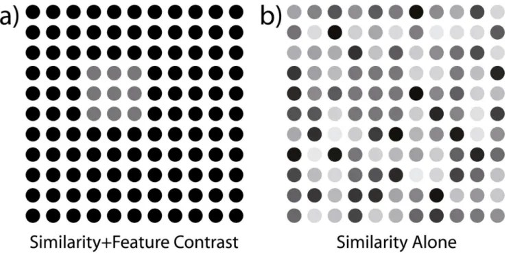
Fig 1. Comparison of grouping cues.(a) illustrates the combination of element similarity and luminance contrast to make the foreground figure visible, (b) removes the feature contrast but adds variability among background elements while keeping the mean luminance of foreground and background equal. Luminance variability is sampled uniformly from the entire interval of available luminance values.
corrected to normal vision. The students had no former psychophysical experience in contour integration.
Ethics statement
Prior to the experiment, participants were informed about the course and expected duration of the experiment. They received a general description of the purpose of the experiment but not about specific outcome expectations. All participants signed a written consent form according to the World Medical Association Helsinki Declaration and were informed that they could withdraw from the experiment at any time without penalty. At the time of data collection, no local ethics committee was instated. Noninvasive experimental studies without deception did not require a formal ethics review provided the experiment complied with the relevant institu-tional and nainstitu-tional regulations and legislation which was carefully ascertained by the authors. After completing the experiment, a summary of their individual data was shown to the observ-ers and the results pattern explained within the scope of the purpose of the study.
Stimuli
Stimulus displays consisted of approximatelynC+nBG= 170 Gabor micropatterns defined by
gðx;yÞ ¼ exp
x2þy2 2s2
sinð2pfðxcosðoÞ ysinðoÞÞÞ: ð1Þ
In (Eq 1) leto¼ φ
180p, withφthe rotation angle measured in degrees. Spatial phase altered ran-domly between even and odd sines. Gabor micropatterns were spatially limited to a diameter of 1.4° visual angle by setting the standard deviationσof the Gaussian envelope to 0.28° and clipping beyond a radius of 2.5σ-units. Random sampling of carrier spatial frequenciesf
started at values not lower than 1.0 cycles per degree (cpd) in all experimental conditions. The defined Gabor size thus kept bandwidths of low frequency micropatterns confined within rea-sonable intervals.
Target contours encompassednC= 12 Gabor elements with an inter-element angle of ±30°,
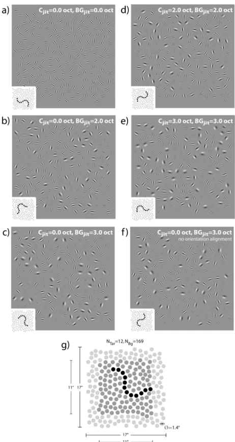
embedded in fields of randomly oriented background elements. Contour shapes ranged from a regular or mirrored“S”to a“U”type figure with outwardly bound tails.Fig 2shows examples of possible contour shapes. The bounding box of a contour always fell within a 11° × 11° square region around the center of the whole 17° × 17° background lattice (seeFig 2g). This limitation was introduced to prevent contours from extending too far into the peripheral field where con-tour integration is known to cease [53].
Construction of target stimuli fell into four steps. First, a contour path was constructed as a smooth trajectory of disjoint elements [6]. Second, background positions were arranged as a hexagonal grid and superimposed onto the contour. Background elements that overlapped contour elements were removed from the grid. Third, a perturbation method [54] was used to randomly displace background element positions. Finally, Gabor elements were placed on all positions. Each background element was assigned a random orientation while contour ele-ments were initially coaligned with the global path trajectory. Carrier spatial frequencies were sampled for both background and contour elements depending on experimental condition. Creation of distracter stimuli adhered to the same procedure, only with the elements of the em-bedded contour also assuming random orientations.
estimated prior to the experiment from Delaunay triangulations [57] of 25.000 patterns con-taining only background positions. Post-hoc analysis of stimuli used during the experiment showed that stimuli exhibited near identical distributions of contour, contour-to-background, and background-to-background element distances. Hence, not only were first-order density cues practically absent from our stimuli [58] but the whole distribution of spatial distances of contour element positions approximated that of background elements.
Orientation jitter in the background was always maximal, samplingφuniformly from the interval [0°;360°]. Detectability of target contours was then modulated by rotating the orienta-tion of Gabor elements away from perfect collinearity by a given tilt angleθ. Increasing values ofθproduce perceptually more and more jagged contours and diminish contour detection per-formance while keeping the global curvature of the path intact. The absolute value ofθwas fixed for any particular contour visibility level, with only the sign alternating randomly. In ac-cordance with observations from previous studies, contours such as used in our experiment be-come undetectable at aboutjθj 30° [59].
Spatial Frequency Variation
There were five conditions of spatial frequency jitter plus two supplemental conditions control-ling for saliency effects due to spatial frequency similarity alone. To have spatial frequency jitter follow a perceptually uniform random distribution we defined spatial frequencies on an octave scale asf= 2u. Depending on experimental condition, the parameteruwas sampled from a uni-form distribution with varying lower and upper limits. Limits were chosen such that the ex-pected value of the resulting exponential distribution wasf ¼3:36cpd in all cases. Stimulus
examples for thefive spatial frequency jitter conditions with orientation defined contours are shown in Fig2a–2e, one of the control conditions with similarity defined contours is depicted inFig 2f.
• C0.0BG0.0—Spatial frequency was constant for both contour and background elements (fC= fBG= 3.36 cpd).
• C0.0BG2.0—Spatial frequency was constant along the contour (fC= 3.36) and randomly
sam-pled for background elements spanning a 2.0 octaves wide interval (fBG¼ ½1:5; 6:2cpd).
• C0.0BG3.0—Same as the previous condition but with background jitter spanning a 3.0 octaves wide interval (fBG= [1;8] cpd).
• C2.0BG2.0—Spatial frequencies were randomly sampled from a 2.0 octaves wide interval for both contour and background (fC¼fBG¼ ½1:5; 6:2cpd).
• C3.0BG3.0—Same as the previous condition but with a 3.0 octaves wide jitter range (fC=fBG=
[1;8] cpd).
• Controls—C0
:0BG2:0andC
0:0BG3:0were the two control conditions, again with either a 2.0 or 3.0 octaves wide sampling interval for carrier spatial frequencies of background elements.
in both the background and along the contour have random orientations, contour elements are homogenous in carrier spatial frequency while background elements exhibit jitter (3.0 octaves in the example shown here). Contour saliency may thus emerge only due to spatial frequency homogeneity. The expected value of the spatial frequency distribution in all jitter conditions isf ¼3:36.
Contour elements had homogenous spatial frequencies but orientations randomly tilted away from perfect collinearity. Hence, in both control conditions, contour detection could no longer rest on orientation alignment but only on spatial frequency similarity among con-tour elements.
Elimination of artificial target cues
In conditions with spatial frequency jitter along the contour, at least every third contour ele-ment was algorithmically set to deviate from its predecessor by more than3
4of the maximum spatial frequency jitter range. This prevented an accidental formation of long chains of ele-ments with similar spatial frequency values along the contour.
During pretesting we noticed that in both control conditions many subjects managed to de-tect a target stimulus significantly above chance level while being incapable of reporting the ac-tual shape of the contour. Further testing revealed that subjects based responses on the perception of unusually high densities of mid-range spatial frequencies (i.e., around 3.36 cpd) in the potential target area which could only occur in target stimuli. To counter this artificial target saliency, we devised a twofold solution. First, for each distracter stimulus appearing in C0.0BG2.0and C0.0BG3.0trials,n= 12 random Gabor elements within the target area were as-signed a spatial frequency off= 3.36 cpd. Second, prior to each stimulus presentation, a spatial frequency shift value was randomly sampled from an interval of [0.0;0.25] octaves and added to all Gabor elements in the respective stimulus, thereby increasing observer uncertainty about the overall spatial frequency mean across stimulus presentations.
Apparatus
Stimuli were generated on a ViSaGe system manufactured by Cambridge Research Systems and displayed on a Samsung 959NF color monitor. The mean luminance of the screen was 50 cd/m2. Stimuli were displayed with a fixed Michelson contrast of 0.95. Color values were taken from a linear grey staircase consisting of 255 steps chosen from a palette of 4096 possible grey values. The relation between grey level entries and the luminance on the screen was linearized by means of gamma correction tables. Linearity was checked before the experiment using a Cambridge Research Systems ColorCAL colorimeter. The determination coefficient of the re-gression line exceededr2= .98 in all cases. The refresh rate of the monitor was 80 Hz at a hori-zontal frequency of 84.62 kHz, the pixel resolution was set to 1348 × 1006 pixels. The ambient illumination of the darkened room approximately matched the illumination on the screen. Pat-terns were viewed binocularly at a distance of 70 cm. Subjects used a chin rest for head stabili-zation and gave their responses with their dominant hand via an external response keyboard.
Psychophysical task
Preliminary measurements and main experiment
Measurement of contour integration performance proceeded in two steps, both of which em-ployed the method of constant stimuli. Initially, contour detection was measured individually for each experimental condition and subject. Detection rates were recorded on five tilt anglesθ at 32 repetitions, and fitted with a Gaussian distribution function of the general form
Fðy;my;syÞ ¼1
1
4 1þerf
y my ffiffiffi 2 p
sy !
" #
ð2Þ
where erf denotes the error function. The two parametersμθandσθwere estimated with the Levenberg-Marquardt algorithm [60]. The parameterμθof the Gaussian distribution function defined in (Eq 2) serves as a direct estimate of the.75 detection threshold from 2AFC measure-ments, the parameterσθis inversely proportional to the slope of the psychometric function, with smaller values ofσθindicating steeper psychometric curves. Note that estimated detection performanceF(θ) is supposed to decrease with increasing tilt angleθ. Hence, ahigherthreshold valueμθdenotesbettervisibility of a contour since it retains saliency until higher tilt values.
Two psychometric functions with sufficient fit were obtained from each condition and sub-ject, whereupon individual sets of five tilt angles were extrapolated. Tilt angles were selected to yield detection rates of 0.59, 0.67, 0.75, 0.83, and 0.91 for each subject in the respective condi-tion. In the main experiment these sets of tilt angles for all experimental conditions were ran-domly intermixed at 32 repetitions for each angle. The implementation of a main experiment that, in principle, differed from the preliminary measurements only by complete randomiza-tion of trials may seem superfluous at first glance. We nonetheless opted for a dedicated main experiment in order to preempt any response bias, stemming from condition specific detection strategies devised by subjects. Analyses, however, proved that the pattern of results from the main experiment closely reflected results from calibration measurements, only at a slightly lower overall performance level. Data analyses rest on two performance measures, tilt angle thresholdμθ, defined as the 0.75 point of the psychometric function, and the standard deviation σθof said function.
Measuring detection rates at 5 tilt angles, each with 32 replications for 5 target conditions plus two control conditions with only one random tilt angle had each subject undergo 864 trials in the main experiment. Together with the preliminary measurements each subject completed at least 2464 trials during the whole experiment. Trials were administered in two sessions on separate days with sufficient warmup trials and one brief intermittent pause. Annotated analy-sis data are provided in fileS1 Dataset.
Results
Psychometric functions
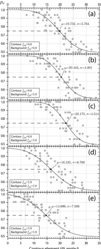
Psychometric function data from the main experiment are summarized inFig 3. Data points represent proportion correct values for all subjects at the respective tilt angleθ. A generalized psychometric function is displayed with parametersμθandσθaveraged across subjects.
Fig 3. Psychometric functions.Fits are depicted separately for all five combinations of contour and background spatial frequency jitter. Data points represent proportion correct measures from all subjects at multiple tilt anglesθ. For each experimental condition a summary psychometric curve is drawn (solid line). The curve is a cumulative Gaussian function intersecting at the between subject mean tilt angle threshold,my,
and with a mean standard deviation estimate,sy. Mean estimates are highlighted by black dots.
Statistical testing
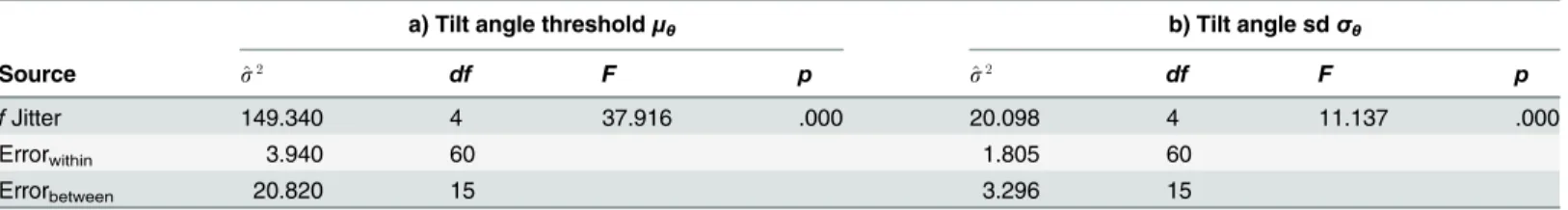
Tilt angle threshold and standard deviation estimates derived from psychometric function data were analyzed by separate repeated measures ANOVAs (rmANOVA). The five variants of con-tour and background spatial frequency jitter served as repeated measures factor levels. The two control conditions is analyzed at a later stage.Table 1summarizes the results of the univariate analyses for both dependent measures,Fig 4illustrates the major findings.
Detection performance. Jitter conditions exert a highly significant effect on contour inte-gration performance (Table 1a). Contour visibility increases when spatial frequency jitter is added to background elements but not contour elements (seeFig 4a). While background jitter of 2.0 octaves does not suffice to elevate thresholds by a statistically significant margin, visibility of homogenous contours significantly benefits from 3.0 octaves spatial frequency jitter in the background. Planned pairwise contrasts of C0.0BG3.0are significant against both previous jitter
Table 1. rmANOVA results for tilt angle thresholdsμθand tilt angle standard deviationsσθ.
a) Tilt angle thresholdμθ b) Tilt angle sdσθ
Source ^s2 df F p ^s2 df F p
fJitter 149.340 4 37.916 .000 20.098 4 11.137 .000
Errorwithin 3.940 60 1.805 60
Errorbetween 20.820 15 3.296 15
Summarized are the source of variation, estimated population variances, degrees of freedom, theF-statistic, and the significance level. Regardless of insignificant Mauchly tests (χ2(9) = 13.088,p= .159 forμθ;χ2(9) = 8.287,p= .505 forσθ), degrees of freedom were Huynh-Feldt corrected before
calculating p-values (see Lecoutre, 1991).
doi:10.1371/journal.pone.0126449.t001
Fig 4. Main effects from rmANOVA.Depicted are between subject means (a) for tilt angle threshold estimatesμθ, and (b) standard deviation estimatesσθ
for all five combinations of contour (C) and background (BG) carrier spatial frequency jitter. Subscripts denote the jitter level in octaves. The dark grey area represents the upper half of the 95% confidence interval for the probability summation prediction for the 2.0 octaves jitter condition, the light gray area for 3.0 octaves, respectively (see text). Panel (c) shows mean proportion correct rates for the detection of contours defined by just spatial frequency similarity, embedded in backgrounds with spatial frequency jitter of 2.0 or 3.0 octaves magnitude, together with their 95% confidence intervals.
levels (C0.0BG2.0and C0.0BG0.0), each with high effect sizes. On the other end, contour detec-tion thresholds suffer significantly from spatial frequency jitter along the contour. All planned pairwise contrasts between C0.0BG0.0, C2.0BG2.0, and C3.0BG3.0reach significance with moder-ate to very high effect sizes (Fig 4a). Modulation of tilt angle standard deviations depending on jitter condition is highly significant (Table 1b). Increasing the spatial frequency jitter along the contour attenuates the slope of psychometric functions (Fig 4b). Planned pairwise comparisons prove both differences between the conditions with spatial frequency jitter (C2.0BG2.0and C3.0BG3.0) against the homogenous condition (C0.0BG0.0) statistically significant with moderate to high effect sizes. In contrast, leaving the spatial frequency of contour elements constant and introducing jitter only in the surround leads to steeper psychometric curves. Both conditions in question (C0.0BG2.0and C0.0BG3.0) yield significantly higher slopes when compared to the fully homogenous condition. Effect sizes are moderate (seeFig 4b).
Saliency gains. This raises the question whether the observed saliency advantages of ho-mogenous contours in heterogenous surrounds root in specific architectural properties of neu-ral contour integration networks, or may be explained simply by probability summation due to simultaneous integration of orientation aligned contours and grouping of similarity defined contours. The control conditions are a viable means to decide between the two alternatives, for they provide an estimate about contour visibility based on spatial frequency similarity alone. Results from the two control conditions are depicted inFig 4c. Detection rates of similarity de-fined contours are very low, yet not entirely at chance level. Hence, spatial frequency similarity might contribute to the visibility of orientation defined target contours as an independent source of saliency. In such a case of probability summation, a prediction of detection perfor-mance can be derived. LetF0(θ) be the detection rate of a homogenous contour with a given tilt angleθin a homogenous background, andG(u) the detection rate of a homogenous (i.e., simi-larity defined) contour embedded in a background with spatial frequency jitter ofuoctaves. I The detection rate predicted by probability summation after guessing correction then com-putes as
~
F0ðy;uÞ ¼1 ½ð1 F0ðyÞÞð1 GðuÞÞ: ð3Þ
BothF0(θ) andG(u) are available from our data.F0(θ) is the psychometric function estimate from condition C0.0BG0.0, andG(u) is the detection rate from the respective control condition (u= 2.0 oru= 3.0 octaves), both corrected for guessing probability. By setting (Eq 3) equal to.5 and solving forθ, one arrives at a probability summation estimate for the tilt angle threshold in the C0.0BG2.0and C0.0BG3.0conditions. From there, confidence interval limits around the threshold predictions can be constructed based on the standard error of the original estimate of μθ.
These confidence intervals are shown as gray shaded areas inFig 4a. It is apparent that the threshold elevation for both conditions of homogenous contours in heterogenous surrounds (C0.0BG2.0and C0.0BG3.0), when compared to wholly homogenous contour stimuli (C0.0BG0.0), is compatible with the assumption of probability summation between an alignment based con-tour integration mechanism and an independent spatial frequency similarity detector.
homogenous contours embedded in heterogenous surrounds, this is due to steeper psychomet-ric functions and higher tilt angle thresholds, whereas for conditions with fully heterogenous spatial frequencies psychometric functions slopes decline and detection thresholds attenuate. All planned pairwise multivariate contrasts reach statistical significance except for the compar-ison between the two fully heterogenous stimulus conditions (C2.0BG2.0against C3.0BG3.0).
To estimate the efficiency of a detector system, the“variation coefficient”r¼s
mcan be com-puted as the ratio of standard deviation to mean parameter [61]. If the variation coefficient is constant across different mean parameters, the standard deviation of the underlying distribu-tion rises propordistribu-tional to the mean parameter. This propordistribu-tionality is a common behaviour of many psychometric variables, such as mental test scores [62]. In sensory analysis constancy of the variation coefficient was observed in simple discrimination tasks under various conditions [63,64], indicating a detector that operates at a constant signal to noise ratio [65]. Larger values of the variation coefficient imply stronger internal noise at the detection criterion, and there-fore less efficient detection [66]. An important implication of constancy of the variation coeffi -cient is parallelism of psychometric functions on log-intensity scales [67]. If the Weibull model is used for the psychometric curve, log-parallelism is obtained if the slope parameterβis con-stant. In addition, regardless of whether the Weibull model or a Gaussion model is used for the
Fig 5. Joint effects of spatial frequency jitter on tilt angle threshold and tilt angle standard deviation.Panel (a) depicts centroids defined by tilt angle thresholdμθ(x-component) and standard deviation estimateσθ(y-component), together with the 95% confidence limits of each component. p-Values are
taken from planned multivariate contrasts between the connected centroids.
psychometric curve, constancy of the variation coefficient implies log-parallelism, indicating the same detector efficiency over a range of stimulus parameters [66]. Analysing the slope pa-rameter for various cases that go beyond a linear systems approach can distinguish between plausible cases of sensory integration and decisional strategy [68], i.e., channel uncertainty and probability summation among channels with additive and multiplicative noise. Since the slope parameter can also be used to estimate the power of the nonlinear signal transducer [69,70], it is widely used to evaluate detection models that involve signal uncertainty [71].
Applied to our data, the variation coefficient can capture an important relationship between psychometric function slope and threshold. If an additional similarity cue yields a higher cer-tainty in detecting orientation defined contours, the increased signal-to-noise ratio should re-sult in higher slopes of psychometric curves for the same mean parameters and thus smaller variation coefficients. Spatial frequency jitter along the contour on the other hand ought to im-pair detection certainty and result in shallower psychometric functions. The uncertainty arising from the necessity of monitoring multiple spatial frequency bands across a large stimulus field for potential target contours has long been known to reduce performance remarkably [72,73]. Fig 6proves the importance of feature uncertainty in contour detection experiments. A sharp increase of the variation coefficientρoccurs for conditions with spatial frequency noise along the contour, indicating a disadvantageous signal (i.e., contour) to noise (i.e., background) rela-tion in such stimuli. In contrast, when similarity is available as a second cue to an alignment defined contour, variation coefficients become smaller, denoting a gain in certainty about
Fig 6. Variation coefficients.Coefficients are computed asr¼sy
my. The parametersσθandμθare taken from psychometric functionfitting, as described in
methods.
contour presence or absence. This gives rise to the conclusion that the similarity principle not so much affects the contour detection process itself but primarily reduces observer uncertainty about whether a potential candidate really is a contour or just a false positive.
Discussion
Results show that contour integration based on orientation collinearity does benefit from simi-larity cues but only in orders of magnitude expected from probability summation between in-dependent saliency mechanisms. This suggests functional independence of the two involved grouping mechanisms. One mechanism integrates contour elements based on orientation col-linearity, the other evaluates similarity relations among stimulus patches. Such functional inde-pendence of the contour integration mechanism from other saliency generating processes has already been found in previous experiments on the combination of orientation alignment with supplemental cues such as motion [41] and color [74]. It shall be noted, though, that the mean tilt angle threshold for the high jitter condition lies in close proximity to the upper bound of the probability summation prediction.
Variability of spatial frequencies along the contour not only affects detection thresholds but the steepness of psychometric functions. The certainty at which contours are detected deterio-rates with increasing jitter along the contour, and grows when similarity cues are added to the contour. Spatial frequency similarity among contour elements in cluttered background appar-ently reinforces the observer’s decision about contour presence in a stimulus. Considering our stimulus arrangements, it can be reasoned that a potential benefit for the integration of homog-enous contour elements in surrounds with spatial frequency variation is overshadowed by higher feature uncertainty of the observer, who needs to scrutinize the stimulus for potential contour candidates in multiple spatial frequency bands simultaneously. The penalty in target detection due to the spread of attention across multiple spatial frequency bands is known to re-duce performance significantly [72,75], and might thus have mediated certainty conditions at the decision stage. Our data support this argument. Although spatial frequency similarity fails to facilitate contour integration by a margin beyond probability summation, it does exert a striking effect on psychometric function slopes. When both contour defining principles— simi-larity and orientation collinearity—are combined along the contour, psychometric functions steepen, and flatten when contour elements jitter in carrier frequencies, as reflected by the vari-ation coefficient.
Despite its potentially beneficial effects on observer certainty, similarity as such does not qualify as a particularly strong figure cue on its own. In accordance with earlier findings [39] contours defined by spatial frequency similarity in heterogenous surrounds proved nearly in-visible, with detection rates only barely exceeding chance level even in the highest jitter condi-tions. We take that as evidence to suggest the absence of specialized cortical networks for similarity driven form completion in cluttered images, rendering local orientation collinearity the key feature for establishing contour saliency.
Psychometric function data further reveal that for small tilt angles, contour integration ap-proaches perfect performance for almost all subjects even in the highest spatial frequency jitter conditions. These figures reinforce the notion of contour integration as a robust shape detec-tion mechanism [39] which integrates not only over a broad range of spatial frequencies but, as recently shown, also over other disruptive factors like large inter-element distances, temporal flicker, or colour and luminance disparities [79].
To link adjacent segments of coaligned stimulus elements, the contour integration mecha-nism may exploit the outputs of orientation detectors with broad spatial frequency tuning, or, alternatively, sum over the outputs of multiple scale-selective detector populations [27]. There is ample evidence that area V1 harbors all necessary means for full-fledged contour integration [12,79,80], possibly aided by feedback connections from higher visual areas [81,82]. More-over, saliency benefits due to multiple cues can be explained by low-level mechanisms for bot-tom-up salience located as early as V1 [83]. A variety of studies have, however, extended our understanding of contour integration by highlighting specific characteristics of human contour integration which might exceed the functional properties of V1 cells. Contour integration is binocular in nature [84], remains functional when presented under conditions of binocular dis-parity between contour elements [38,43], combines multiple scales [39,76], and works on sti-muli devoid of luminance modulation such as collinear bars of isoluminant color [85].
Integration across spatial frequency, across eyes, and through color hints at the contribution of other visual areas besides V1. One candidate is area V2 where cells with all necessary properties have been found [86]. Electrophysiological and neuroimaging studies have further diversified our picture of the locus of contour integration. Their findings implicate ventral regions like the parietal cortex, inferio-temporal cortex (IT), and the lateral occipital complex (LOC) in the grouping of contour parts into outlines of figures and shapes on larger scales [30,32,87]. Re-cent studies attempted to reconcile the different, partly opposing views of early versus late im-plementation of contour integration routines. Contour dependent activation appears to be tightly coupled between multiple cortical levels. While an initial peak of contour related activa-tion has been found in area V4, delayed but congruent activaactiva-tion followed on V1, probably modulated by inter-area feedback projections [31]. Taken together, it is likely that contour in-tegration and form completion involve multiple processing levels with mutual interactions along the neural processing stream [88–90]. The results of the present study help to highlight specific characteristics of such a contour integration mechanism with respect to the effects of spatial frequency variation.
Supporting Information
S1 Dataset. The files included in the ZIP archive provide the dataset on which all statistical analyses were conducted, annotations to connect the dataset with the names and labels used in the article, and a legend to explain naming conventions.
(ZIP)
Author Contributions
Conceived and designed the experiments: MP GM. Performed the experiments: MP GM. Ana-lyzed the data: MP GM. Contributed reagents/materials/analysis tools: MP GM. Wrote the paper: MP GM.
References
2. Beck J (1972) Similarity grouping and peripheral discriminability under uncertainty. American Journal of Psychology 85: 1–19. doi:10.2307/1420955PMID:5019427
3. Bergen JR, Adelson EH (1988) Early vision and texture perception. Nature 333: 363–364. doi:10. 1038/333363a0PMID:3374569
4. Landy MS, Bergen JR (1991) Texture segregation and orientation gradient. Vision Res 31: 679–691. doi:10.1016/0042-6989(91)90009-TPMID:1843770
5. Rubenstein BS, Sagi D (1990) Spatial variability as a limiting factor in texture-discrimination tasks: im-plications for performance asymmetries. J Opt Soc Am A 7: 1632–1643. doi:10.1364/JOSAA.7. 001632PMID:2213287
6. Field DJ, Hayes A, Hess RF (1993) Contour integration by the human visual system: Evidence for a local“association field”. Vision Res 33: 173–193. doi:10.1016/0042-6989(93)90156-QPMID:
8447091
7. Wertheimer M (1958) Principles of perceptual organization, Princeton: Van Nostrand.
8. Kovacs I (2000) Human development of perceptual organization. Vision Res 40: 1301–1310. doi:10. 1016/S0042-6989(00)00055-9PMID:10788641
9. Baker TJ, Tse J, Gerhardstein P, Adler SA (2008) Contour integration by 6-month-old infants: discrimi-nation of distinct contour shapes. Vision Res 48: 136–148. doi:10.1016/j.visres.2007.10.021PMID:
18093632
10. Gervan P, Berencsi A, Kovacs I (2011) Vision first? the development of primary visual cortical networks is more rapid than the development of primary motor networks in humans. Plos One 6. doi:10.1371/ journal.pone.0025572PMID:21984933
11. Kovacs I, Julesz B (1993) A closed curve is much more than an incomplete one: Effect of closure in fig-ure-ground segmentation. Proc Natl Acad Sci U S A 90: 7495–7497. doi:10.1073/pnas.90.16.7495
PMID:8356044
12. Hess RF, Field D (1999) Integration of contours: New insights. Trends Cogn Sci 3: 480–486. doi:10. 1016/S1364-6613(99)01410-2PMID:10562727
13. Rockland KS, Lund JS (1983) Intrinsic laminar lattice connections in primate visual-cortex. Journal of Comparative Neurology 216: 303–318. doi:10.1002/cne.902160307PMID:6306066
14. Malach R, Amir Y, Harel M, Grinvald A (1993) Relationship between intrinsic connections and function-al architecture revefunction-aled by opticfunction-al imaging and in vivo targeted biocytin injections in primate striate cor-tex. Proc Natl Acad Sci U S A 90: 10469–10473. doi:10.1073/pnas.90.22.10469PMID:8248133
15. Schmidt KE, Goebel R, Lowel S, Singer W (1997) The perceptual grouping criterion of colinearity is re-flected by anisotropies of connections in the primary visual cortex. Eur J Neurosci 9: 1083–1089. doi:
10.1111/j.1460-9568.1997.tb01459.xPMID:9182961
16. Rockland KS, Lund JS, Humphrey AL (1982) Anatomical binding of intrinsic connections in striate cor-tex of tree shrews (tupaia glis). J Comp Neurol 209: 41–58. doi:10.1002/cne.902090105PMID:
7119173
17. Ng J, Bharath AA, Zhaoping L (2007) A survey of architecture and function of the primary visual cortex (v1). Eurasip Journal on Advances in Signal Processing. doi:10.1155/2007/97961
18. Stettler DD, Das A, Bennett J, Gilbert CD (2002) Lateral connectivity and contextual interactions in ma-caque primary visual cortex. Neuron 36: 739–750. doi:10.1016/S0896-6273(02)01029-2PMID:
12441061
19. Gilbert CD, Wiesel TN (1989) Columnar specificity of intrinsic horizontal and corticocortical connections in cat visual cortex. J Neurosci 9: 2432–2442. PMID:2746337
20. Kinoshita M, Gilbert CD, Das A (2009) Optical imaging of contextual interactions in v1 of the behaving monkey. J Neurophysiol 102: 1930–1944. doi:10.1152/jn.90882.2008PMID:19587316
21. Shmuel A, Korman M, Sterkin A, Harel M, Ullman S, et al. (2005) Retinotopic axis specificity and selec-tive clustering of feedback projections from v2 to v1 in the owl monkey. J Neurosci 25: 2117–2131. doi:
10.1523/JNEUROSCI.4137-04.2005PMID:15728852
22. Bosking WH, Zhang Y, Schofield B, Fitzpatrick D (1997) Orientation selectivity and the arrangement of horizontal connections in tree shrew striate cortex. J Neurosci 17: 2112–2127. PMID:9045738
23. Polat U, Mizobe K, Pettet MW, Kasamatsu T, Norcia AM (1998) Collinear stimuli regulate visual re-sponses depending on cell’s contrast threshold. Nature 391: 580–584. doi:10.1038/35372PMID:
9468134
25. Roelfsema PR, Lamme VA, Spekreijse H (2004) Synchrony and covariation of firing rates in the primary visual cortex during contour grouping. Nat Neurosci 7: 982–991. doi:10.1038/nn1304PMID:
15322549
26. Gilad A, Meirovithz E, Leshem A, Arieli A, Slovin H (2012) Collinear stimuli induce local and cross-areal coherence in the visual cortex of behaving monkeys. PLoS One 7: e49391. doi:10.1371/journal.pone. 0049391PMID:23185325
27. Gilad A, Meirovithz E, Slovin H (2013) Population responses to contour integration: Early encoding of discrete elements and late perceptual grouping. Neuron 78: 389–402. doi:10.1016/j.neuron.2013.02. 013PMID:23622069
28. Nowak LG, Bullier J (1997) The timing of information transfer in the visual system, New York: Plrenum Press, volume 12 ofCerebral Cortexpp. 205–241.
29. Mandon S, Kreiter AK (2005) Rapid contour integration in macaque monkeys. Vision Res 45: 291–
300. doi:10.1016/j.visres.2004.08.010PMID:15607346
30. Shpaner M, Molholm S, Forde E, Foxe JJ (2013) Disambiguating the roles of area V1 and the lateral oc-cipital complex (LOC) in contour integration. Neuroimage 69: 146–156. doi:10.1016/j.neuroimage. 2012.11.023PMID:23201366
31. Chen MG, Yan Y, Gong XJ, Gilbert CD, Liang HL, et al. (2014) Incremental integration of global con-tours through interplay between visual cortical areas. Neuron 82: 682–694. doi:10.1016/j.neuron. 2014.03.023PMID:24811385
32. Mijovic B, De Vos M, Vanderperren K, Machilsen B, Sunaert S, et al. (2014) The dynamics of contour in-tegration: A simultaneous eeg-fmri study. Neuroimage 88C: 10–21. doi:10.1016/j.neuroimage.2013. 11.032
33. Dakin SC, Baruch NJ (2009) Context influences contour integration. J Vis 9: 1–13. doi:10.1167/9.2.13
34. Beaudot WH, Mullen KT (2003) How long range is contour integration in human color vision? Vis Neu-rosci 20: 51–64. doi:10.1017/S0952523803201061PMID:12699083
35. Schumacher JF, Quinn CF, Olman CA (2011) An exploration of the spatial scale over which orientation-dependent surround effects affect contour detection. J Vis 11: 12. doi:10.1167/11.8.12PMID:
21778251
36. Bex PJ, Simmers AJ, Dakin SC (2001) Snakes and ladders: the role of temporal modulation in visual contour integration. Vision Research 41: 3775–3782. doi:10.1016/S0042-6989(01)00222-XPMID:
11712989
37. Mullen KT, Beaudot WH, McIlhagga WH (2000) Contour integration in color vision: a common process for the blue-yellow, red-green and luminance mechanisms? Vision Res 40: 639–655. doi:10.1016/ S0042-6989(99)00204-7PMID:10824267
38. Hess RF, Field DJ (1995) Contour integration across depth. Vision Res 35: 1699–1711. doi:10.1016/ 0042-6989(94)00261-JPMID:7660578
39. Persike M, Olzak LA, Meinhardt G (2009) Contour integration across spatial frequency. J Exp Psychol Hum Percept Perform 35: 1629–1648. doi:10.1037/a0016473PMID:19968425
40. Mathes B, Trenner D, Fahle M (2006) Do subthreshold colour-cues increase contour detection perfor-mance?, Lengerich: Pabst Science Publishers. p. 82.
41. Ledgeway T, Hess RF, Geisler WS (2005) Grouping local orientation and direction signals to extract spatial contours: Empirical tests of“association field”models of contour integration. Vision Res 45: 2511–2522. doi:10.1016/j.visres.2005.04.002PMID:15890381
42. Machilsen B, Wagemans J (2011) Integration of contour and surface information in shape detection. Vi-sion Res 51: 179–186. doi:10.1016/j.visres.2010.11.005PMID:21093469
43. Hess RF, Hayes A, Kingdom FA (1997) Integrating contours within and through depth. Vision Res 37: 691–696. doi:10.1016/S0042-6989(96)00215-5PMID:9156213
44. Meinhardt G, Persike M, Mesenholl B, Hagemann C (2006) Cue combination in a combined feature contrast detection and figure identification task. Vision Res 46: 3977–3993. doi:10.1016/j.visres.2006. 07.009PMID:16962156
45. Persike M, Meinhardt G (2006) Synergy of features enables detection of texture defined figures. Spat Vis 19: 77–102. doi:10.1163/156856806775009214PMID:16411484
46. Persike M, Meinhardt G (2008) Cue summation enables perceptual grouping. J Exp Psychol Hum Per-cept Perform 34: 1–26. doi:10.1037/0096-1523.34.1.1PMID:18248137
47. Yen SC, Finkel LH Identification of salient contours in cluttered images. In: Computer Vision and Pat-tern Recognition. IEEE Computer Society, pp. 273–279.
48. Li Z (1998) A neural model of contour integration in the primary visual cortex. Neural Comput 10: 903–
49. Hansen T, Neumann H (2008) A recurrent model of contour integration in primary visual cortex. J Vis 8. doi:10.1167/8.8.8
50. Ernst UA, Mandon S, Schinkel-Bielefeld N, Neitzel SD, Kreiter AK, et al. (2012) Optimality of human contour integration. PLoS Comput Biol 8: e1002520. doi:10.1371/journal.pcbi.1002520PMID:
22654653
51. Green DM, Swets JA (1988) Signal detection theory and psychophysics. Los Altos: Wiley.
52. Tversky T, Geisler WS, Perry JS (2004) Contour grouping: Closure effects are explained by good con-tinuation and proximity. Vision Res 44: 2769–2777. doi:10.1016/j.visres.2004.06.011PMID:
15342221
53. Hess RF, Dakin SC (1997) Absence of contour linking in peripheral vision. Nature 390: 602–604. doi:
10.1038/37352PMID:9403687
54. Braun J (1999) On the detection of salient contours. Spat Vis 12: 211–225. doi:10.1163/ 156856899X00120PMID:10221428
55. Kovacs I (1996) Gestalten of today: Early processing of visual contours and surfaces. Behav Brain Res 82: 1–11. doi:10.1016/S0166-4328(97)81103-5PMID:9021065
56. Gervan P, Kovacs I (2010) Two phases of offline learning in contour integration. Journal of Vision 10. doi:10.1167/10.6.24PMID:20884573
57. Lee DT, Schachter BJ (1980) Two algorithms for constructing a Delaunay triangulation. International Journal of Parallel Programming 9: 219–242.
58. Kozma-Wiebe P, Silverstein SM, Feher A, Kovacs I, Ulhaas P, et al. (2006) Development of a world-wide web based contour integration test. Computers in Human Behavior 22: 971–980. doi:10.1016/j. chb.2004.03.017
59. Roudaia E, Bennett PJ, Sekuler AB (2013) Contour integration and aging: the effects of element spac-ing, orientation alignment and stimulus duration. Front Psychol 4: 356. doi:10.3389/fpsyg.2013.00356
PMID:23801978
60. Marquardt D (1963) An algorithm for least-squares estimation of nonlinear parameters. SIAM Journal on Applied Mathematics 11: 431–441. doi:10.1137/0111030
61. Crozier WJ (1936) On the sensory discrimination of intensities. Proc Natl Acad Sci U S A 22: 412–416. doi:10.1073/pnas.22.6.412PMID:16588097
62. Lord FM, Novick MR (1968) Statistical theories of mental test scores. Reading: Addison-Wesley. 63. Crozier WJ, Holway AH (1937) On the law for minimal discrimination of intensities: I. Proc Natl Acad Sci
U S A 23: 23–28. doi:10.1073/pnas.23.1.23PMID:16577762
64. Blackwell HR (1963) Neural theories of simple visual discriminations. J Opt Soc Am 53: 129–160. doi:
10.1364/JOSA.53.000129PMID:13971408
65. Roufs JA (1974) Dynamic properties of vision. IV. Thresholds of decremental flashes, incremental flashes and doublets in relation to flicker fusion. Vision Res 14: 831–851. doi:10.1016/0042-6989(74) 90148-5PMID:4422125
66. Mortensen U, Suhl U (1991) An evaluation of sensory noise in the human visual system. Biol Cybern 66: 37–47. doi:10.1007/BF00196451PMID:1768711
67. Mortensen U (1988) Visual contrast detection by a single channel versus probability summation among channels. Biol Cybern 59: 137–147. doi:10.1007/BF00317776PMID:3207771
68. Tyler CW, Chen CC (2000) Signal detection theory in the 2afc paradigm: attention, channel uncertainty and probability summation. Vision Res 40: 3121–3144. doi:10.1016/S0042-6989(00)00157-7PMID:
10996616
69. Nachmias J, Sansbury RV (1974) Letter: Grating contrast: discrimination may be better than detection. Vision Res 14: 1039–1042. doi:10.1016/0042-6989(74)90175-8PMID:4432385
70. Meinhardt G (1999) Evidence for different nonlinear summation schemes for lines and gratings at threshold. Biol Cybern 81: 263–277. doi:10.1007/s004220050561PMID:10473850
71. Wallis SA, Baker DH, Meese TS, Georgeson MA (2013) The slope of the psychometric function and non-stationarity of thresholds in spatiotemporal contrast vision. Vision Res 76: 1–10. doi:10.1016/j. visres.2012.09.019PMID:23041562
72. Kramer P, Graham N, Yager D (1985) Simultaneous measurement of spatial-frequency summation and uncertainty effects. J Opt Soc Am A 2: 1533–1542. doi:10.1364/JOSAA.2.001533PMID:
4045585
74. Mathes B, Fahle M (2007) Closure facilitates contour integration. Vision Res 47: 818–827. doi:10. 1016/j.visres.2006.11.014PMID:17286999
75. Kingdom FA, Keeble DR (2000) Luminance spatial frequency differences facilitate the segmentation of superimposed textures. Vision Res 40: 1077–1087. doi:10.1016/S0042-6989(99)00233-3PMID:
10738067
76. Dakin SC, Hess RF (1999) Contour integration and scale combination processes in visual edge detec-tion. Spatial Vision 12: 309–327. doi:10.1163/156856899X00184PMID:10442516
77. Taylor CP, Bennett PJ, Sekuler AB (2014) Evidence for adjustable bandwidth orientation channels. Frontiers in Psychology 5: 578. doi:10.3389/fpsyg.2014.00578PMID:24971069
78. Taylor CP, Bennett PJ, Sekuler AB (2009) Spatial frequency summation in visual noise. J Opt Soc Am A Opt Image Sci Vis 26: B84–B93. doi:10.1364/JOSAA.26.000B84PMID:19884918
79. Hall S, Bourke P, Guo K (2014) Low level constraints on dynamic contour path integration. PLoS One 9: e98268. doi:10.1371/journal.pone.0098268PMID:24932494
80. Giersch A, Humphreys GW, Boucart M, Kovacs I (2000) The computation of occluded contours in visual agnosia: Evidence for early computation prior to shape binding and figure-ground coding. Cognitive Neuropsychology 17: 731–759. doi:10.1080/026432900750038317PMID:20945203
81. Das A, Gilbert CD (1999) Topography of contextual modulations mediated by short-range interactions in primary visual cortex. Nature 399: 655–661. doi:10.1038/21371PMID:10385116
82. Bredfeldt CE, Ringach DL (2002) Dynamics of spatial frequency tuning in macaque V1. J Neurosci 22: 1976–1984. PMID:11880528
83. Zhaoping L, Zhe L (2012) Properties of v1 neurons tuned to conjunctions of visual features: application of the v1 saliency hypothesis to visual search behavior. PLoS One 7: e36223. doi:10.1371/journal. pone.0036223PMID:22719829
84. Huang PC, Hess RF, Dakin SC (2006) Flank facilitation and contour integration: Different sites. Vision Res 46: 3699–3706. doi:10.1016/j.visres.2006.04.025PMID:16806389
85. McIlhagga WH, Mullen KT (1996) Contour integration with colour and luminance contrast. Vision Res 36: 1265–1279. doi:10.1016/0042-6989(95)00196-4PMID:8711906
86. Wilson HR, Wilkinson F (1997) Evolving concepts of spatial channels in vision: from independence to nonlinear interactions. Perception 26: 939–960. doi:10.1068/p260939PMID:9509156
87. Altmann CF, Bülthoff HH, Kourtzi Z (2003) Perceptual organization of local elements into global shapes in the human visual cortex. Curr Biol 13: 342–349. doi:10.1016/S0960-9822(03)00052-6PMID:
12593802
88. Kourtzi Z, Kanwisher N (2000) Cortical regions involved in perceiving object shape. J Neurosci 20: 3310–3318. PMID:10777794
89. Lerner Y, Hendler T, Ben-Bashat D, Harel M, Malach R (2001) A hierarchical axis of object processing stages in the human visual cortex. Cereb Cortex 11: 287–297. doi:10.1093/cercor/11.4.287PMID:
11278192
90. Kourtzi Z, Huberle E (2005) Spatiotemporal characteristics of form analysis in the human visual cortex revealed by rapid event-related fMRI adaptation. Neuroimage 28: 440–452. doi:10.1016/j.