Response of the AMOC to reduced solar radiation – the modulating role of atmospheric chemistry

www.earth-syst-dynam.net/7/877/2016/ doi:10.5194/esd-7-877-2016

© Author(s) 2016. CC Attribution 3.0 License.

Response of the AMOC to reduced solar radiation –

the modulating role of atmospheric chemistry

Stefan Muthers1,2,a, Christoph C. Raible1,2, Eugene Rozanov3,4, and Thomas F. Stocker1,2 1_{Climate and Environmental Physics, University of Bern, Bern, Switzerland}

2_{Oeschger Centre for Climate Change Research, University of Bern, Bern, Switzerland} 3_{Institute for Atmospheric and Climate Science, ETH, Zurich, Switzerland}

4_{Physikalisch-Meteorologisches Observatorium Davos and World Radiation Center (PMOD/WRC),}

Davos, Switzerland

a_{now at: German Meteorological Service, Research Center Human Biometeorology, Freiburg, Germany}

Correspondence to:Stefan Muthers (muthers@climate.unibe.ch)

Received: 15 April 2016 – Published in Earth Syst. Dynam. Discuss.: 25 April 2016 Revised: 30 September 2016 – Accepted: 22 October 2016 – Published: 11 November 2016

Abstract. The influence of reduced solar forcing (grand solar minimum or geoengineering scenarios like solar radiation management) on the Atlantic Meridional Overturning Circulation (AMOC) is assessed in an ensemble of atmosphere–ocean–chemistry–climate model simulations. Ensemble sensitivity simulations are performed with and without interactive chemistry. In both experiments the AMOC is intensified in the course of the solar radiation reduction, which is attributed to the thermal effect of the solar forcing: reduced sea surface temperatures and enhanced sea ice formation increase the density of the upper ocean in the North Atlantic and intensify the deepwater formation. Furthermore, a second, dynamical effect on the AMOC is identified driven by the stratospheric cooling in response to the reduced solar forcing. The cooling is strongest in the tropics and leads to a weakening of the northern polar vortex. By stratosphere–troposphere interactions, the stratospheric circulation anomalies induce a negative phase of the Arctic Oscillation in the troposphere which is found to weaken the AMOC through wind stress and heat flux anomalies in the North Atlantic. The dynamic mechanism is present in both ensemble experiments. In the experiment with interactive chemistry, however, it is strongly amplified by stratospheric ozone changes. In the coupled system, both effects counteract and weaken the response of the AMOC to the solar forcing reduction. Neglecting chemistry–climate interactions in model simulations may therefore lead to an overestimation of the AMOC response to solar forcing.

1 Introduction

The Atlantic Meridional Overturning Circulation (AMOC) is an important component of climate variability in the North Atlantic region (Kuhlbrodt et al., 2007; Stocker, 2013). The surface branch of the AMOC transports heat from the South-ern Hemisphere (SH) and the tropics towards the north, is closely connected to the Atlantic Multidecadal Oscillation, and contributes to the temperate climatic conditions in west-ern Europe (Knight et al., 2006). Thus, understanding the variations in the strength of this circulation is important in particular for future climate change (Stocker and

Schmit-tner, 1997; Manabe and Stouffer, 1999; Mikolajewicz and Voss, 2000; Gregory et al., 2005), decadal climate predic-tions (Griffies and Bryan, 1997; Meehl et al., 2009), and with respect to potential abrupt climatic changes as proposed for the past (Stocker and Wright, 1991; Stocker, 2000; Clark et al., 2002).

inves-TSI anomaly (Wm

−

2)

G

lo

b

a

l m

e

a

n

2

m

t

e

m

p

e

ra

tu

re

(

K

)

(a) TSI forcing

(b) Global mean 2 m temperatures

(c) AMOC

CTRL S1 (-3.5 Wm-2₎ S2 (-20 Wm-2₎

CHEM NOCHEM

S1 (-3.5 Wm-2₎ S2 (-20 Wm-2₎

Simulation years ●

● ● ●

●● ●

●●

●●●●●●●●●●●●●● ●●●●

●● ●●

● ●●●

●● ●●●

●●●●●●●●●●

●●

●

●

● ● ● ●

●

Figure 1.(a)Total solar irradiance (TSI) anomaly of−3.5 Wm−2(dashed) and−20 Wm−2(solid) applied in this study.(b)Global annual

mean ensemble mean 2 m temperature.(c)Ensemble mean AMOC index in the different experiments, smoothed using a 5-year running mean. Dots denote significant differences in the (un-smoothed) annual mean values between the SRR ensemble and the control ensemble (Student’sttest,p≤0.05). Small stars below the CHEM time series correspond to years with significant differences between the CHEM and NOCHEM experiment (p≤0.05). The beginning and the end of the SRR period are indicated by vertical lines in panels(b)and(c).

tigate the role of chemistry–climate interactions in modulat-ing the response of the atmospheric circulation to reduced solar radiation and their effect on the AMOC. To this end, we perform ensemble sensitivity simulations for different so-lar radiation reductions (SRRs) with a state-of-the-art cou-pled atmosphere–ocean–chemistry–climate model, where at-mospheric chemistry is either enabled or disabled.

So far, the external forcing response of the AMOC has been mainly studied in climate models without interactive at-mospheric chemistry (Otterå et al., 2010). Thereby, volcanic eruptions have been found to intensify the AMOC on decadal timescales (Otterå et al., 2010; Mignot et al., 2011), through a reduction in sea surface temperatures and a shift of the North Atlantic Oscillation (NAO) towards its positive phase. Moreover, volcanic eruptions may excite the variability in the AMOC (Swingedouw et al., 2015). The response, however, may depend on the background conditions of the climate sys-tem (Zanchettin et al., 2012). An increase in the solar

forc-ing has been found to weaken the AMOC by increasforc-ing sea surface temperatures (SSTs) and enhancing freshwater in-put (Cubasch et al., 1997; Latif et al., 2009; Otterå et al., 2010; Swingedouw et al., 2011) and has been proposed to be a driver of Greenland temperature variations (Waple et al., 2002; Kobashi et al., 2015).

1999, 2001; Thompson and Wallace, 2001) and may also af-fect the AMOC (Manzini et al., 2012; Reichler et al., 2012). The stratospheric response to UV variations is modu-lated by chemistry–climate interactions (Haigh, 1994, 1996). In particular, stratospheric ozone reacts to solar irradiance changes. The increase in solar UV enhances the shortwave heating rate through ozone absorption (e.g. Forster et al., 2011). Additional solar UV in the Herzberg continuum

(λ <242 nm) intensifies ozone production, while UV in the

Hartley band destroys ozone (e.g. Ball et al., 2016, Fig. 1). Because the solar UV variability decreases with wavelength the first effect prevails and leads to ozone increase in the mid-dle stratosphere in phase with the increase in the solar UV. In turn the ozone increase gives additional heating with mag-nitude comparable to primary heating by the increase in so-lar UV alone (Forster et al., 2011). This process can amplify the efficiency of the earlier mentioned top-down propagation (Kodera and Kuroda, 2002) and is obviously missing if the ozone concentration is prescribed.

Still, most of these studies are based on models with-out interactive atmospheric chemistry. The influence of cli-mate changes on the state of the ozone layer has long been recognized. The cooling of the stratosphere by greenhouse gases (GHGs) slows down catalytic ozone oxidation cy-cles, leading to ozone increase (e.g. Haigh and Pyle, 1982; Revell et al., 2012). The greenhouse warming accelerates Brewer–Dobson circulation reducing ozone in the tropical lower stratosphere and enhancing its abundance over middle to high latitudes (Deckert and Dameris, 2008; Zubov et al., 2013). The ozone changes have substantial implications for the climate. The influence of the ozone recovery associated with the implementation of the Montreal Protocol limita-tions on the production of ozone destroying substances on the SH has been identified in observations and model simu-lations (e.g. Son et al., 2008; Robinson and Erickson, 2015). Recently, it was suggested that the use of interactive chem-istry instead of prescribed ozone climatology can influence climate model properties. Dietmüller et al. (2014) showed that the application of interactive chemistry reduces the mate sensitivity by 3–8 %. A similar reduction in the cli-mate sensitivity was also found by Muthers et al. (2014b). A more substantial reduction in the model response to 4×CO₂ by up to 20 % due to taking into account interactive chem-istry was reported by Nowack et al. (2014). All these stud-ies attributed the reduction to the changes in ozone, water vapour, and clouds in response to climate warming. These conclusions were not confirmed by very recent results of the CESM1-WACCM model (Marsh et al., 2016), which found a similar ozone response to 4×CO2but no changes in cli-mate sensitivity. In contrast, Chiodo and Polvani (2016) ap-plied the same model and demonstrated that the interactive ozone introduces a negative feedback leading to a weaker surface warming due to an enhancement of the solar irradi-ance. Thus, these results show that further experiments are necessary in order to assess the model discrepancies and to

deepen our understanding of the ozone feedback and its im-portance for the simulation of future climate change under the influence of different natural and anthropogenic factors.

The outline of this study is as follows. The model configu-ration and the experiments are described in Sect. 2. Section 3 presents the results, first for the experiments without interac-tive atmospheric chemistry and then through an analysis of the differences causes by the chemistry–climate interactions. A summary and concluding discussion is given in Sect. 4.

2 Model and experiments

2.1 The model

We use the coupled atmosphere–ocean–chemistry model SOCOL-MPIOM to simulate the effect of a change in so-lar activity on the climate (Muthers et al., 2014b). SOCOL (Stenke et al., 2013) consists of the atmospheric compo-nent ECHAM5 (Roeckner et al., 2003) coupled to the chem-istry module MEZON (Rozanov et al., 1999; Egorova et al., 2003). The middle-atmospheric configuration of ECHAM5 is used (Manzini et al., 2006), which resolves the atmo-sphere up to 0.01 hPa (about 80 km) with 39 levels. The hor-izontal resolution is T31, corresponding to a grid size of 3.75◦

×3.75◦.

The chemistry is directly coupled to ECHAM5 and uses temperature data to calculate the tendency of 41 gas species, taking into account 200 gas-phase, 16 heterogeneous, and 35 photolytical reactions. Optionally, the coupling to MEZON can be disabled. In this case a three-dimensional time-dependent ozone data set needs to be specified.

The shortwave radiation scheme of SOCOL considers spectral solar irradiance (SSI) values in six spectral bands. Time series for each spectral interval are used as forcing to allow for changes in the spectral composition of the total solar irradiance. The shortwave scheme considers Rayleigh scattering, scattering on aerosols and clouds, and the ab-sorption of UV by O2, O3, and 44 other species. Additional parametrizations for the absorption of UV in the Lyman-alpha, Schumann–Runge, Hartley, and Higgins bands are im-plemented following Egorova et al. (2004) and Sukhodolov et al. (2014). The longwave scheme considers wavenum-bers between 10 and 3000 cm−1_{and takes into account} wa-ter vapour, CO2, O3, N2O, CH4, CFC-11, CFC-12, CFC-22, aerosols, and clouds.

With the given vertical resolution, SOCOL is not able to produce a Quasi-Biennial Oscillation (QBO). Thus, a QBO nudging is applied (Giorgetta et al., 1999). The time step of the atmospheric component is 15 min, with the full radiation and chemical computations updates performed every 2 h.

shifted and placed over land (Greenland and central Antarc-tica). The nominal resolution is 3◦_{– varying between 22 and} 350 km – with a higher resolution in the deep water formation regions in the North Atlantic and the Weddell Sea. Convec-tion is implemented by greatly enhanced vertical diffusion when the water column becomes unstable. Sea ice dynamics are based on the viscous–plastic rheology formulated by Hi-bler (1979). A constant sea ice salinity of 5 psu is assumed. The time step of the oceanic component is 2 h and 24 min.

2.2 The experiments

Ensemble sensitivity simulations with SOCOL-MPIOM are performed to study the effect of SRR on the climate system and the AMOC. Such SRRs are caused by either a grand so-lar minimum or soso-lar radiation management techniques. Ten simulations are carried out for each ensemble experiment; the experiments differ in the solar forcing applied and whether or not chemistry–climate interactions are considered in the model.

Perpetual AD 1600 conditions and zero volcanic aerosols (i.e. excluding the volcanic eruption of Huaynaputina) are applied in all simulations. For the sensitivity simulations only the solar forcing is allowed to change in time. The solar forc-ing consists of the SSI and photolysis rates.

As reference experiment we perform two control ensem-bles, CTRL_CHEM and CTRL_NOCHEM, with and with-out interactive chemistry, respectively. In these experiments all forcings represent the conditions of the year AD 1600, including the solar forcings of the year AD 1600. The year 1600 was chosen since a stable long-term control simulation with SOCOL-MPIOM was available from previous studies (Anet et al., 2013a, 2014; Muthers et al., 2014b). Note that the differences in the climatic conditions between 1600 and the commonly used year 1850 are small and both represent a pre-industrial climate state.

The two SRRs simulated for this study are character-ized by a step-wise total solar irradiance (TSI) reduction of −3.5 and−20 Wm−2_{, referred to as S1 and S2, respectively} (Fig. 1a). The S1 SRR is comparable to a grand solar minima like the Dalton minimum or Maunder minimum in a large-amplitude solar forcing reconstruction (e.g. Shapiro et al., 2011). With−20 Wm−2_{the S2 SRR is comparable to a weak} solar radiation management scenario (Kravitz et al., 2011), which may counteract an increase in the radiative forcing from GHGs of about 3 Wm−2_{. The reduction in the solar} forcings is switched on at year 5 of a simulation and lasts for 30 years when it is switched off and the simulation is contin-ued for 25 years. Both SRRs are simulated with and without interactive chemistry and are named S1_CHEM, S2_CHEM, S1_NOCHEM, and S2_NOCHEM in the following. A sum-mary of the experiments performed for this study is given in Table 1.

In the CHEM experiments, ECHAM5 and MEZON are coupled and the atmospheric chemistry responds to the

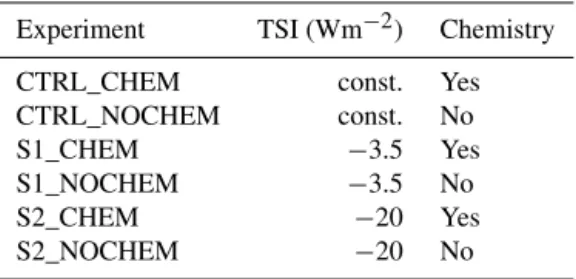
so-Table 1.Overview of the ensemble experiments used in this study.

Each ensemble consists of 10 experiments.

Experiment TSI (Wm−2_{) Chemistry}

CTRL_CHEM const. Yes

CTRL_NOCHEM const. No

S1_CHEM −3.5 Yes

S1_NOCHEM −3.5 No

S2_CHEM −20 Yes

S2_NOCHEM −20 No

lar radiation changes. In NOCHEM, temporal and spatial ozone variations need to be prescribed. Therefore, a daily 3-D ozone climatology is applied, based on a A3-D 1600 control simulations.

All ensemble simulations are initialized from model year 1300 of a long control simulation with interactive chemistry performed under perpetual AD 1600 conditions (Muthers et al., 2014b). The ensemble members only differ in their ini-tial conditions by slightly perturbing the atmosphere (atmo-spheric restarts for 1, 2, 3 January, etc.). The oceanic compo-nent is always initialized using the same initial conditions.

Note that we erroneously applied a slightly different so-lar forcing in 6 of 10 simulations. This TSI difference of 0.018 Wm−2 _{is caused by a different rounding of the SSI} values and leads to very small differences between the con-trol ensemble experiments and the SRR experiments already prior to the start of the reduction.

3 Results

Both SRRs lead to a significant reduction in the global mean near-surface (2 m) air temperature (Fig. 1b). For the stronger S2 experiment the cooling is more pronounced than for the S1 experiments and reaches −1.0 and −0.9 K for S2_CHEM and S2_NOCHEM, respectively (averaged over the last 5 years of the SRR period). For the S1 experiment, the temperatures reduce by −0.1 K in both ensembles. The temperature instantaneously responds to the imposed radia-tion drop and reaches the lowest values at the end of the re-duction period. The continuous cooling in the course of the SRR, which is well visible in the S2 ensembles, suggests that the model has not yet reached thermal equilibrium. In fact, from the model’s equilibrium climate sensitivity (for a dou-bling of CO2, see Muthers et al., 2014b) an equilibrium tem-perature response of−1.3 K is expected for S2_CHEM and −1.4 K for S2_NOCHEM. However, a comparison with the CO2 sensitivity is only a rough estimate, since the climate sensitivity (and the contributions from chemistry–climate in-teractions) differs between the solar and CO2forcing and de-pends on the sign of the forcing perturbation (Hansen et al., 1997; Schaller et al., 2014).

The larger cooling in the CHEM experiments is related to differences in the stratospheric response. In particular, strato-spheric ozone concentrations are reduced due to the reduced UV radiation (Fig. S1a, d in the Supplement), a process which is not considered in the NOCHEM experiments. Ad-ditionally, water vapour concentrations are affected by the SRR. In S2_NOCHEM, the largest anomalies (−15 %) are found in the tropical upper troposphere, but stratospheric re-ductions exceed−10 % almost everywhere (Fig. S1c in the Supplement). In S2_CHEM, the stratospheric reductions in water vapour are more pronounced (up to−35 %), due to the effect of the solar forcing on the oxidation of methane, the most important in situ source of stratospheric water vapour (Fig. S1b in the Supplement). Due to the greenhouse effect of ozone and water vapour, the outgoing longwave flux in-creases more in CHEM than in the NOCHEM and leads to an additional cooling of the troposphere. The positive wa-ter vapour anomalies found in the uppermost model levels in the CHEM experiments (Fig. S1b, e in the Supplement) are related to the reduced UV photolysis of the water vapour molecules.

A slight initial reduction in the global mean temperature is also found in the reference ensemble experiments and is related to the initial conditions of the ocean. With all ensem-ble simulations sharing the same oceanic conditions in the beginning, the AMOC development of the first years is dom-inated by the oceanic memory. During the first decade of the experiments a decline in the AMOC from 21.0 to 19.8 Sv is found (Fig. 1c). This decline is very similar in both reference experiments. The minimum state of the AMOC is reached in year 12–13 of the reference experiments and in the

fol-lowing years the AMOC increases to its maximum value of 21.4 Sv in year 35.

The AMOC is not affected by the SRR during the first few years of the simulation. Starting with simulation year 10, however, and even more pronounced in the second half of the reduction period, the AMOC is significantly stronger in S1_NOCHEM during several years and in S2_NOCHEM for most of the years between years 15 and 35 of the ex-periment. In the CHEM ensemble simulations no significant AMOC intensification is found for S1. In S2_CHEM, the AMOC is significantly stronger during the second half of the SRR period, but the intensification is weaker in comparison to S2_NOCHEM. The differences between the AMOC in-dex for S2_CHEM and S2_NOCHEM are also reflected in the anomaly pattern of the AMOC (Fig. S2 in the Supple-ment). Within the first 10 years the intensification of the cir-culation is weak. Positive anomalies are found between 40 and 65◦_{N and between the surface and a depth of 2800 m} depth. During these first 20 years of the reduction period the intensification is slightly larger in S2_CHEM. A pronounced strengthening of the circulation occurs in the second decade of the reduction period. Positive anomalies cover all latitudes from the Equator to 65◦_{N and most levels between the} sur-face and 3000 m depth. In the second decade the intensifi-cation is more pronounced in S2_NOCHEM. In the third decade, finally, a further intensification is found, which is again stronger in S2_NOCHEM. In the following, we will first address the relevant processes that are responsible for the AMOC intensification (Sect. 3.1) before we assess the role of chemistry–climate interactions in order to explain the lower sensitivity of the AMOC to SRR in the CHEM experi-ments (Sect. 3.2).

3.1 The thermal effect of SRR on the AMOC

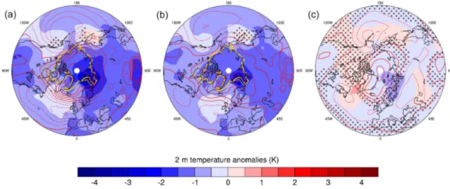
A direct effect of SRR is the reduction in shortwave energy reaching the troposphere and the surface and thus in tem-perature, which is apparent almost everywhere in the NH (Fig. 2). Averaged over the 30-year reduction period the sea ice growth in the Barents Sea is stronger in S2_CHEM than in S2_NOCHEM (Fig. 2). Furthermore, a larger cooling over the Barents Sea is found in S2_CHEM, which extends to-wards northern Eurasia. In the S1 experiments temperature and sea ice anomaly patterns are weaker but similar to S2 and S1_CHEM is characterized by an amplified cooling as well (not shown). During the first 10 years, when no AMOC differences between the CHEM and NOCHEM experiments are found, the temperature and sea ice anomalies are very similar. The Arctic sea ice differences between CHEM and NOCHEM, which emerge in the last 20 years of the reduc-tion period, are therefore related to the weaker AMOC in the CHEM experiments and the reduced heat transport into the Arctic.

temper-Figure 2.Annual mean 2 m temperature anomalies (colours), sea level pressure anomalies (red contours), and 50 % sea ice extent line (yellow contours) averaged over the SRR period. Temperature and sea level pressure anomalies are calculated relative to the control ensemble mean; for the sea ice extent, the values of the control ensemble and the S2 experiments are depicted by the solid and dashed line, respectively. Panel(a)shows the difference for the S2_CHEM ensemble, and the S2_NOCHEM anomalies are shown in(b). Panel (c)displays the differences between S2_CHEM and S2_NOCHEM. Dots denote non-significant temperature differences (Student’sttest,p >0.05). The sea level pressure contour interval is 0.25 hPa and negative sea level pressure anomalies are dashed.

atures and an increased salinity due to the enhanced sea ice formation, the density of the upper ocean increases al-most everywhere (Fig. 3a–i). Additionally, a shift of the storm track and a significant reduction in the precipitation in the North Atlantic contributes to the salinity and den-sity increase (not shown). During the first 10 years of the SRR period, differences in the density anomalies in the up-per ocean of the North Atlantic are small and not signifi-cant, except for a region south of Greenland, where the den-sity is significantly higher in S2_NOCHEM (Fig. 3a–c). In the following decade further increases in the upper ocean density are found in both experiments, but the anomalies are again larger in S2_NOCHEM (Fig. 3d–f). During this time, the density anomalies in large parts of the North At-lantic are more pronounced in S2_NOCHEM in comparison to S2_CHEM. Finally, in the last 10 years, density anomalies are still strongly positive, but the differences between both experiments weaken (Fig. 3g–i).

Convection takes place in the Nordic Seas and in a re-gion in the North Atlantic close to the Labrador Sea (con-tours in Fig. 3e–h). The intensity of the deep water forma-tion in these two regions is an important driver of AMOC variability (Jungclaus et al., 2005). Focusing on the changes in the Nordic Seas, we find an intensification of the deep water formation already for the first 10 years of the reduc-tion period (Fig. 3j–l). A further intensificareduc-tion is found for the second and the third decade, but the anomalies between S2_CHEM and S2_NOCHEM show only weak significance. The anomalies in the S1 experiments are similar – i.e. dif-ferences are mostly non-significant. Density changes in the Nordic Seas are driven by a combination of temperature and salinity changes (Fig. 4). The temperature changes, however,

dominate in the first half of the SRR period, while the in-creasing salinity drives the density changes in the second half.

In the North Atlantic the density and mixed layer dif-ferences between S2_CHEM and S2_NOCHEM are larger than the ones in the Nordic Seas. During the first 10 years of the SRR period, positive mixed layer depth anomalies are found in S2_NOCHEM (Fig. 3k), while no consistent response is found in S2_CHEM (Fig. 3j). Consequently, the intensification is significantly stronger in S2_NOCHEM (Fig. 3l). A similar picture emerges for the second decade (Fig. 3m–o). In the third decade a clear intensification is obvious in S2_CHEM, while a slight reduction is found in S2_NOCHEM in the southern region of the North Atlantic convection zone (Fig. 3p–r). As in the Nordic Seas, the den-sity changes are driven by the reduced temperatures in the first half of the SRR (Fig. 4). In the second half of the SRR period the salt content of the upper ocean increases, while temperatures increase again, related to the intensification of the overturning. The salinity changes, nevertheless, lead to a further increase in the density in the second half of the re-duction period.

Figure 3.(a–i)S2_CHEM(a, d, g), S2_NOCHEM(b, e, h), and the difference between S2_CHEM and S2_NOCHEM(c, f, i)ensemble mean upper ocean (0–220 m) density anomalies (kg m−3_{) for late winter (January–March) averaged over the first(a–c), second(d–f), and} last decade(g–i)of the SRR period. Cyan contours display the extent of the 50 % sea ice area for the CTRL ensemble mean (solid line) and the SRR experiments (dashed line). Panels(j–r): S2_CHEM(j, m, p), S2_NOCHEM(k, n, q), and the difference between S2_CHEM and S2_NOCHEM(l, i, r)ensemble mean January–March mixed layer depth anomalies (m, shading) averaged over the first(j–l), second

(m–o), and last decade(p–r)of the SRR period. Contours denote the average January–March mixed layer depth in CTRL_CHEM and CTRL_NOCHEM, with a contour step of 500 m. Dots denote non-significant density or mixed layer depth differences (Student’st test,

p >0.05).

therefore needed to understand the differences in the AMOC response between the CHEM and NOCHEM experiments.

3.2 The dynamical effect and the role of chemistry–climate interactions

Chemistry–climate interactions are most pronounced in the stratosphere (e.g. Dietmüller et al., 2014). In particular, the different response of the stratospheric ozone and water

1026.95 ₁₀₂₇

1027.05 1027.1

1027.15 1027.2

34.35 34.40 34.45 34.50 34.55 34.60

5.6

5.8

6.0

6.2

6.4

6.6

Salinity (psu)

T

emper

ature (K)

North Atlantic

Salinity (psu)

T

emper

ature (K)

North Atlantic

1027.35 1027.4 1027.45

1027.5 1027.55

1027.6

1027.65

34.65 34.70 34.75 34.80 34.85 34.90 34.95 35.00

4.0

4.5

5.0

Salinity (psu)

T

emper

ature (K)

Nordic Seas

Salinity (psu)

T

emper

ature (K)

Nordic

Figure 4.Temperature and salinity averaged over the upper 220 m for two deep water formation regions: the North Atlantic and Nordic Seas.

The deep water formation regions cover all grid cells with an annual mean mixed layer depth≥250 m in the corresponding ocean basins. The lines show the salinity and temperature development from the beginning (triangle) to the end (large dot) of the SRR for the S2_CHEM (orange) and S2_NOCHEM (blue) experiments. Each point represents a single year. To improve visibility, the values are smoothed using a 15-year low-pass filter. Error bars denote the mean and the standard deviation of the corresponding control ensembles. Contours represent the water density.

Figure 5.Annual mean zonal mean temperature(a–c)and annual mean zonal mean zonal wind(d–f)anomalies in the S2 experiments

(a)

(b)

(c)

(d)

E E

Figure 6.(a, b)Ensemble mean number of sudden stratospheric warming (SSW) events per winter season (November–March) as in defined

by Charlton and Polvani (2007).(c, d)Box plot statistics for the number of SSW events per winter season averaged over the SRR period. The beginning and the end of the SRR period are indicated by vertical lines in panels(a)and(b).

ing in S2_NOCHEM is much smaller than the response in S2_CHEM (Fig. 5b, c). Furthermore, as a consequence of the missing response of the ozone concentrations to the re-duced solar forcing, the effect of the lower- and middle-stratospheric cooling on the meridional temperature gradient is weaker.

The response of the zonal mean wind in the stratosphere agrees well with the temperature anomalies. For S2_CHEM, a pronounced weakening of the NH and SH polar vortices is found (Fig. 5d–f). Using the zonal mean wind compo-nent at 60◦_{N and 10 hPa as an index for the intensity of} the NH polar vortex (Christiansen, 2001, 2005), a reduc-tion of−43 % is found in S2_CHEM during the winter sea-son (November–March) when averaged over the SRR period. The largest wind anomalies occur during the vortex maxi-mum in January. The reduction in S2_NOCHEM is much weaker (−8 %) than in S2_CHEM. Furthermore, the dura-tion of the winter period with predominant westerly wind is reduced in S2_CHEM by−30 % and in S2_NOCHEM by −5 %, respectively, when defining the start of the winter pe-riod by the day with the first occurrence of a westerly daily mean zonal mean wind component at 60◦_{N and 10 hPa after} September and the end by the first day with easterly winds after March. Qualitatively similar results are found for the S1 experiments, with November–March vortex anomalies of −9 % for S1_CHEM and−2 % for S1_NOCHEM (Fig. S3 in the Supplement). These responses highlight the non-linear relationship between the solar forcing and the atmospheric dynamics.

The weakening of the NH polar vortex is closely re-lated to the occurrence of sudden stratospheric warming (SSW) events (Fig. 6). SSW events are stratospheric ex-treme events in which the westerly flow during winter time

is reversed and a strong warming in the polar stratosphere is observed. SSW events in the NH are associated with a breakdown of the polar vortex. Following the SSW defini-tion by Charlton and Polvani (2007), almost a doubling of the number of SSW events is found in S2_CHEM (1.34 events per winter in comparison to 0.68 events per winter in CTRL_CHEM). In S1_CHEM an increase to 0.73 events is simulated. Similarly to the NH polar vortex, the effect of the SRR on the SSW events is small in NOCHEM. For S1 the average number of events increases from 0.68 events per winter in CTRL_NOCHEM to 0.70 events per winter in S1_NOCHEM. In S2_NOCHEM an increase to 0.73 events is simulated. While the increase in the mean number of SSW events is small in S2_NOCHEM, a clear reduction in the years with a low number of SSW events is found (lower quartile of the box plot).

The NH polar vortex and extreme events like SSW af-fect the tropospheric circulation in the NH by stratosphere– troposphere interactions. A downward propagation of wind speed anomalies from the middle stratosphere to the surface is related to positive and negative phases of the AO (Baldwin and Thompson, 2009). For a negative phase of the AO, neg-ative wind anomalies in the stratosphere occur up to 40 days before the AO event takes place at the surface (Fig. S4 in the Supplement). For a positive phase of the AO, the zonal wind anomalies are even stronger (not shown). Overall, the down-ward propagation of wind speed anomalies does not differ substantially between the CHEM and NOCHEM control ex-periments.

Arc-0 10 20 30 40 50

Year

A

O inde

x (standardiz

ed)

● ● ●

●

●

●

−1.0

−0.5

0.0 0.5 1.0

● ●● ●● ●●●

● ● ●

● ●

● ●

● ●

−1.0

−0.5

0.0 0.5 1.0

●

●

CTRL S1 S2

● CTRL S1 S2 S1 (-3.5 Wm-2

) S2 (-20 Wm-2₎

CHEM NOCHEM

(a)

(b)

(c)

(d)

Figure 7. (a, b)Ensemble mean AO index (standardized and reversed sea level pressure difference between 45 and 65◦_{N) per winter}

(November–March). Dots indicate winters with significant differences to the CTRL ensemble (Student t testp≤0.05).(c, d)Box plot statistics for the AO index averaged over the SRR. The beginning and the end of the SRR period are indicated by vertical lines in panels

(a)and(b).

tic and negative anomalies in the North Atlantic and the North Pacific, similar to a negative phase of the AO. In S2_NOCHEM, comparable negative and positive pressure patterns are found, but the anomalies are much weaker (Fig. 2b). Due to the strength of the response, the winter phe-nomenon AO is reflected in the annual mean values (Fig. 2). However, when focusing on the winter season (November– March) and the AO index, the strength of the anomalies in S2_CHEM is even more apparent (Fig. 7). During the entire SRR phase a persistent negative phase of the AO is found in S2_CHEM. In S1_CHEM the tendency towards a nega-tive AO is found as well, although the response is weaker and several years with a positive phase of the AO occur dur-ing the SRR. In the NOCHEM experiments the response is in general weaker, but a shift towards a negative AO phase from CTRL_NOCHEM to S1_NOCHEM and S2_NOCHEM is apparent (Fig. 7d). In particular, negative AO phases tend to occur more often in the first half of the SRR period, while neutral conditions dominate in the second half.

Atmospheric chemistry–climate interactions therefore lead to pronounced differences in the dynamical response to the SRR, from the stratosphere down to the surface of the NH high latitudes. With a shift in the pressure pattern which affects the wind systems in the lower atmosphere, these dif-ferences have the potential to also modify the oceanic circu-lation.

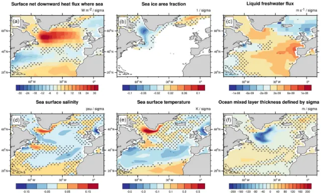
The control experiments are used to assess the influence of the AO phase on the North Atlantic. Regressing the AO index on different oceanic variables reveals that a nega-tive AO phase is associated with an increased downward heat flux south of Greenland and negative heat flux

anoma-lies close to the east coast of North America during win-ter in CTRL_CHEM (Fig. 8a). Sea ice cover is reduced in the Labrador Sea (Fig. 8b) and the dynamical changes lead to an increased total freshwater flux into large parts of the North Atlantic, as well as a reduced flux in the Nordic Seas (Fig. 8c). These changes cause a reduction in the salin-ity (Fig. 8d), except for a small region south of Greenland, which may be affected by a weakening of the East land Current. Additionally, SSTs increase south of Green-land (Fig. 8e), related to the enhanced downward heat flux. Since the density of the water decreases with increasing tem-perature and decreasing salinity, all these changes lead to a pronounced reduction in the mixed layer depth (Fig. 8f). In CTRL_NOCHEM the effect of the AO is very similar (Fig. S5 in the Supplement).

These changes at the ocean surface are also reflected in the AMOC index. In both control experiments the AMOC reacts within the same winter season to the AO phase, as de-tected by the positive correlation between the winter AO and the AMOC index of the same season (Fig. S6 in the Supple-ment). Furthermore, the AO phase has long-lasting effect on the overturning, reflected in significant positive correlations for lags up to 9 years.

dynam-Figure 8. Influence of a negative AO phase on different oceanic variables in CTRL_CHEM during winter (November–March). Linear regression coefficients for(a)net downward heat flux,(b)sea ice area fraction,(c)liquid freshwater flux (evaporation minus precipitation),

(d)sea surface salinity,(e)sea surface temperature, and(f)mixed layer depth. To highlight the influence of a negative AO phase, the AO index has been reversed in the regression analysis. Dots denote non-significant temperature differences (Student’sttest,p >0.05).

ical changes decrease the density of the surface ocean wa-ters south of Greenland, reduce convection, and weaken the AMOC. In the NOCHEM experiments a tendency towards a negative phase of the AO is found as well, although less pro-nounced, due to the absence of chemistry–climate interac-tions. The dynamical effect on the AMOC is therefore much weaker and the thermal response dominates.

4 Conclusions and discussions

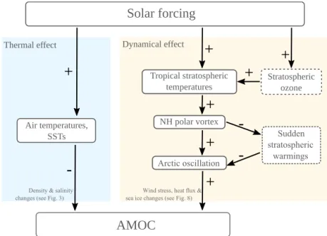
Sensitivity experiments for different solar minima and model configurations with and without chemistry–climate interac-tions have been carried out to study the response of the AMOC to reduced solar forcing and the modulating role of chemistry–climate interactions. Without interactive chem-istry the response of the AMOC is dominated by the direct thermal effect, leading to an intensification of the overturning circulation. A second dynamical effect is identified in the ex-periments with chemistry–climate interactions and leads to a weakening of the overturning.

The two processes are summarized in Fig. 9: the thermal effect is related to the reduced shortwave energy reaching the troposphere and the surface and the ensuing cooling of the lower atmosphere and the upper ocean. This increases the sea surface density and enhances convection. The thermal effect, however, is compensated for by the dynamical effect when atmospheric chemistry is taken into account. Induced by the

reduction in the tropical stratospheric temperatures, a weak-ening of the NH polar vortex and – by interactions between the stratospheric and tropospheric circulation – a negative phase of the AO is found in response to the SRR. The circu-lation changes in the troposphere in turn cause a weakening of the AMOC by anomalous heat and freshwater fluxes. The dynamical effect is amplified by chemistry–climate interac-tions, due to the enhanced stratospheric temperature response related to the effect of the reduced UV radiation on the ozone concentrations. For the weaker S1 SRR, both effects can-cel each other out and therefore no AMOC intensification is found in the experiments with interactive chemistry. In the S2 experiments with stronger forcing, however, the thermal response of the AMOC dominates and the dynamical effect leads only to a reduced intensification of the overturning.

Solar forcing

AMOC

Sudden stratospheric

warmings

Stratospheric ozone Thermal effect

Air temperatures, SSTs

+

Tropical stratospheric temperatures

NH polar vortex

Arctic oscillation

+

+

+

+

+

+

-Dynamical effect

Figure 9.Flowchart summarizing the thermal and dynamical effect of a change in solar radiation on the AMOC. The signs indicate the

correlation between two processes. Dashed boxes represent effects which are amplified by chemistry–climate interactions.

within the next 100 years (Lockwood et al., 2009; Stein-hilber and Beer, 2013; Roth and Joos, 2013), although the amplitude of the TSI changes is associated with large uncer-tainties. While the influence on the global mean temperature increase is small (Feulner and Rahmstorf, 2010; Meehl et al., 2013; Anet et al., 2013b), the thermal effect may reduce the projected 21st century AMOC weakening. This is confirmed by experiments of Anet et al. (2013b). The AMOC is sig-nificantly stronger in the late 21st century in ensemble sim-ulations including a grand solar minimum in comparison to ensemble simulations without a decline in the solar activity (Fig. S7 in the Supplement).

Parts of the dynamical effect have been reported in pre-vious studies. The relationship between solar variability and the stratospheric circulation was found for the 11-year cycle (Kodera and Kuroda, 2002; Mitchell et al., 2015) as well as for grand solar minima (Anet et al., 2013a). The projection of the stratospheric anomalies on the AO has also been re-ported in previous studies (Kodera, 2003; Ineson et al., 2011; Scaife et al., 2013). Finally, the influence of the AO phase on the overturning has been studied (Delworth and Greatbatch, 2000; Eden and Willebrand, 2001; Matthes et al., 2006; Del-worth and Zeng, 2016) and a few studies have identified a possible influence of the stratospheric circulation on the overturning (Manzini et al., 2012; Reichler et al., 2012).

The stratosphere responds very rapidly to the reduced so-lar forcing and the tropospheric AO index shifts to a negative phase in the second winter after the onset of the reduction pe-riod, although it takes about 5 years before a persistent neg-ative AO phase is found in S2_CHEM. The response of the AMOC, however, is delayed by several years. A similar delay was reported by Delworth and Zeng (2016), who performed

sensitivity experiments with an ocean model forced by dif-ferent atmospheric conditions. In one experiment a persis-tent positive phase of the NAO is simulated and the AMOC responds to this forcing with strengthening of the circula-tion, which is delayed by 5–7 years (see Fig. 3 in Delworth and Zeng, 2016). This lag of the response agrees with our results, although an exact timing is difficult to estimate from our setup.

The influence of the dynamic effect on the AMOC may furthermore depend on the length of the solar reduction pe-riod. Lohmann et al. (2009) found a gradual weakening of the subpolar gyre response with time in ocean model simu-lations forced with a persistent negative phase of the NAO. Additionally, the response of the AMOC may be non-linear and an increase in the solar forcing may change the dynamic effect (Lohmann et al., 2009).

Recently, Chiodo and Polvani (2016) assessed the role of the interactive chemistry on the temperature and precipitation response to increasing SSI. They identified a reduced sensi-tivity with interactive chemistry due to the effect of the ozone increase on the shortwave radiation balance. Our results for a SSI reduction indicate a slightly larger temperature sensi-tivity with interactive chemistry owing to the effect of the stratospheric water vapour and ozone changes on the long-wave radiation balance. These differences may be attributed to model differences or differences in the response of the climate system to increasing and decreasing solar forcing. A possible effect of the differences in the atmospheric re-sponse on the AMOC is not discussed by Chiodo and Polvani (2016).

so-lar forcing and identify the importance of chemistry–climate interactions for the response. Hence, previous studies with-out atmospheric chemistry may overestimate the sensitivity of the AMOC to solar forcing since the dynamical effect is absent.

Furthermore, our results reveal possible additional side ef-fects of the solar radiation management technique: a reduc-tion in the incoming solar radiareduc-tion in space to mitigate the temperature increase caused by the emission of GHGs might affect the tropospheric circulation patterns in the NH and cause a weakening of AMOC with climatic consequences, in particular for the temperate climate in western Europe. The dynamical effect is expected to change, however, when the solar radiation is reduced in the Earth’s atmosphere, for instance, by stratospheric sulfate aerosols. In this case, a strengthening of the NH polar vortex and a positive phase of the AO may develop, analogous to the response to strong tropical volcanic eruptions (Graf et al., 1993; Kodera, 1994; Stenchikov et al., 2002; Muthers et al., 2014a, 2015). This effect of the positive AO phase may, in turn, lead to an in-tensification of the AMOC. Future studies should address the influence of stratospheric sulfate geoengineering on the AMOC and the possible role of chemistry–climate interac-tions.

5 Data availability

All simulations described in this study are archived at the University of Bern and are available on request.

The Supplement related to this article is available online at doi:10.5194/esd-7-877-2016-supplement.

Acknowledgements. We thank the four anonymous reviewers

for their constructive comments. This work was supported by the Swiss National Science Foundation under grants CRSII2-147659 (FUPSOL II) and 200020-159563.

Edited by: R. A. P. Perdigão

Reviewed by: four anonymous referees

References

Anet, J. G., Muthers, S., Rozanov, E., Raible, C. C., Peter, T., Stenke, A., Shapiro, A. I., Beer, J., Steinhilber, F., Brönnimann, S., Arfeuille, F., Brugnara, Y., and Schmutz, W.: Forcing of stratospheric chemistry and dynamics during the Dalton Mini-mum, Atmos. Chem. Phys., 13, 10951–10967, doi:10.5194/acp-13-10951-2013, 2013a.

Anet, J. G., Rozanov, E. V., Muthers, S., Peter, T., Brönnimann, S., Arfeuille, F., Beer, J., Shapiro, A. I., Raible, C. C., Steinhilber, F., and Schmutz, W. K.: mpact of a potential 21st century grand solar

minimum on surface temperatures and stratospheric ozone, Geo-phys. Res. Lett., 40, 4420–4425, doi:10.1002/grl.50806, 2013b. Anet, J. G., Muthers, S., Rozanov, E. V., Raible, C. C., Stenke, A.,

Shapiro, A. I., Brönnimann, S., Arfeuille, F., Brugnara, Y., Beer, J., Steinhilber, F., Schmutz, W., and Peter, T.: Impact of solar versus volcanic activity variations on tropospheric temperatures and precipitation during the Dalton Minimum, Clim. Past, 10, 921–938, doi:10.5194/cp-10-921-2014, 2014.

Baldwin, M. P. and Dunkerton, T. J.: Propagation of the Arctic Os-cillation from the stratosphere to the troposphere, J. Geophys. Res., 104, 30937–30946, doi:10.1029/1999JD900445, 1999. Baldwin, M. P. and Dunkerton, T. J.: Stratospheric harbingers

of anomalous weather regimes, Science, 294, 581–584, doi:10.1126/science.1063315, 2001.

Baldwin, M. P. and Thompson, D. W. J.: A critical comparison of stratosphere – troposphere coupling indices, Q. J. Roy. Meteor. Soc., 1672, 1661–1672, doi:10.1002/qj, 2009.

Ball, W. T., Haigh, J. D., Rozanov, E. V., Kuchar, A., Sukhodolov, T., Tummon, F., Shapiro, A. V., and Schmutz, W.: High solar cycle spectral variations inconsistent with stratospheric ozone observations, Nat. Geosci., 9, 206–209, doi:10.1038/ngeo2640, 2016.

Budich, R., Gioretta, M., Jungclaus, J., Redler, R., and Reick, C.: The MPI-M Millennium Earth System Model: An assembling guide for the COSMOS configuration, MPI report, Max-Planck Institute for Meteorology, Hamburg, Germany, 22 pp., 2010. Charlton, A. J. and Polvani, L. M.: A new look at stratospheric

sud-den warmings. Part I: Climatology and modeling benchmarks, J. Climate, 20, 449–470, 2007.

Chiodo, G. and Polvani, L. M.: Reduction of Climate Sensitivity to Solar Forcing due to Stratospheric Ozone Feedback, J. Climate, 29, 4651–4663, doi:10.1175/JCLI-D-15-0721.1, 2016.

Christiansen, B.: Downward propagation of zonal mean zonal wind anomalies from the stratosphere to the troposphere: Model and reanalysis, J. Geophys. Res., 106, 27307, doi:10.1029/2000JD000214, 2001.

Christiansen, B.: Downward propagation and statistical forecast of the near-surface weather, J. Geophys. Res., 110, D14104, doi:10.1029/2004JD005431, 2005.

Clark, P. U., Pisias, N. G., Stocker, T. F., and Weaver, A. J.: The role of thermohaline circulation in abrupt climate change, Na-ture, 415, 863–869, doi:10.1038/415863a, 2002.

Cubasch, U., Voss, R., Hegerl, G. C., Waszkewitz, J., and Crowley, T. J.: Climate dynamics simulation of the influence of solar radi-ation variradi-ations on the global climate with an ocean-atmosphere general circulation model, Clim. Dynam., 13, 757–767, 1997. Deckert, R. and Dameris, M.: Higher tropical SSTs strengthen the

tropical upwelling via deep convection, Geophys. Res. Lett., 35, 2–5, doi:10.1029/2008GL033719, 2008.

Delworth, T. L. and Greatbatch, R. J.: Multidecadal thermo-haline circulation variability driven by atmospheric surface flux forcing, J. Climate, 13, 1481–1495, doi:10.1175/1520-0442(2000)013<1481:MTCVDB>2.0.CO;2, 2000.

Delworth, T. L. and Zeng, F.: The impact of the North Atlantic Oscillation on climate through its influence on the Atlantic Meridional Overturning Circulation, J. Climate, 29, 941–962, doi:10.1175/JCLI-D-15-0396.1, 2016.

simulations, J. Geophys. Res.-Atmos., 119, 1796–1805, doi:10.1002/2013JD020575, 2014.

Eden, C. and Willebrand, J.: Mechanism of interannual to decadal variability of the North Atlantic circula-tion, J. Climate, 14, 2266–2280, doi:10.1175/1520-0442(2001)014<2266:MOITDV>2.0.CO;2, 2001.

Egorova, T., Rozanov, E., Zubov, V., and Karol, I. L.: Model for Investigating Ozone Trends (MEZON), Izvestiya, Atmos. Ocean. Phys., 39, 277–292, 2003.

Egorova, T., Rozanov, E., Manzini, E., Schmutz, W., and T. P.: Chemical and dynamical response to the 11-year variability of the solar irradiance simulated with a chemistry-climate model, Geophys. Res. Lett., 83, 6225–6230, 2004.

Feulner, G. and Rahmstorf, S.: On the effect of a new grand mini-mum of solar activity on the future climate on Earth, Geophys. Res. Lett., 37, L05707, doi:10.1029/2010GL042710, 2010. Forster, P. M., Fomichev, V. I., Rozanov, E., Cagnazzo, C.,

Jon-sson, A. I., Langematz, U., Fomin, B., Iacono, M. J., Mayer, B., Mlawer, E., Myhre, G., Portmann, R. W., Akiyoshi, H., Falaleeva, V., Gillett, N., Karpechko, A., Li, J., Lemennais, P., Morgenstern, O., Oberländer, S., Sigmond, M., and Shibata, K.: Evaluation of radiation scheme performance within chem-istry climate models, J. Geophys. Res.-Atmos., 116, D10302, doi:10.1029/2010JD015361, 2011.

Giorgetta, M. A., Bengtsson, L., and Arpe, K.: An investiga-tion of QBO signals in the east Asian and Indian mon-soon in GCM experiments, Clim. Dynam., 15, 435–450, doi:10.1007/s003820050292, 1999.

Graf, H.-F., Kirchner, I., Robock, A., and Schult, I.: Pinatubo erup-tion winter climate effects: Model versus observaerup-tions, Clim. Dy-nam., 92, 81–93, 1993.

Gregory, J., Dixon, K., Stouffer, R., Weaver, A., Driesschaert, E., Eby, M., Fichefet, T., Hasumi, H., Hu, A., Jungclaus, J., Kamenkovich, I. V., Levermann,A., Montoya, M., Murakami, S.,Nawrath, S., Oka, A., Sokolov, A. P., and Thorpe, R. B.: A model intercomparison of changes in the Atlantic thermohaline circulation in response to increasing atmospheric CO2 concen-tration, Geophys. Res. Lett., 32, L12703, 2005.

Griffies, S. M. and Bryan, K.: Predictability of North At-lantic Multidecadal Climate Variability, Science, 275, 181–184, doi:10.1126/science.275.5297.181, 1997.

Haigh, J. D.: The role of stratospheric ozone in modulating the solar radiative forcing of climate, Nature, 370, 544–546, 1994. Haigh, J. D.: The Impact of Solar Variability on Climate, Science,

272, 981–984, 1996.

Haigh, J. D. and Pyle, J. A.: Ozone perturbation experiments in a two-dimensional circulation model, Q. J. Roy. Meteor. Soc., 108, 551–574, doi:10.1002/qj.49710845705, 1982.

Hansen, J., Sato, M., and Ruedy, R.: Radiative forcing and climate response, J. Geophys. Res., 102, 6831–6864, doi:10.1029/96JD03436, 1997.

Hibler, W. D.: A dynamic thermodynamic sea ice model, J. Phys. Oceanogr., 9, 815–846, 1979.

Ineson, S., Scaife, A. A., Knight, J. R., Manners, J. C., Dunstone, N. J., Gray, L. J., and Haigh, J. D.: Solar forcing of winter cli-mate variability in the Northern Hemisphere, Nat. Geosci., 4, 1– 5, doi:10.1038/ngeo1282, 2011.

Jungclaus, J. H., Haak, H., Latif, M., and Mikolajewicz, U.: Arctic– North Atlantic interactions and multidecadal variability of the

Meridional Overturning Circulation, J. Climate, 18, 4013–4031, doi:10.1175/JCLI3462.1, 2005.

Jungclaus, J. H., Keenlyside, N., Botzet, M., Haak, H., Luo, J.-J., Latif, M., Marotzke, J., Mikolajewicz, U., and Roeck-ner, E.: Ocean circulation and tropical variability in the cou-pled model ECHAM5/MPI-OM, J. Climate, 19, 3952–3972, doi:10.1175/JCLI3827.1, 2006.

Knight, J. R., Folland, C. K., and Scaife, A. A.: Climate impacts of the Atlantic Multidecadal Oscillation, Geophys. Res. Lett., 33, 1–4, doi:10.1029/2006GL026242, 2006.

Kobashi, T., Box, J. E., Vinther, B. M., Goto-Azuma, K., Blu-nier, T., White, J. W. C., Nakaegawa, T., and Andresen, C. S.: Modern solar maximum forced late twentieth cen-tury Greenland cooling, Geophys. Res. Lett., 42, 5992–5999, doi:10.1002/2015GL064764, 2015.

Kodera, K.: Influence of volcanic eruptions on the troposphere through stratospheric dynamical processes in the Northern Hemi-sphere winter, J. Geophys. Res., 99, 1273–1282, 1994.

Kodera, K.: Solar influence on the spatial structure of the NAO during the winter 1900–1999, Geophys. Res. Lett., 30, 1175, doi:10.1029/2002GL016584, 2003.

Kodera, K. and Kuroda, Y.: Dynamical response to the solar cycle, J. Geophys. Res.-Atmos., 107, 4749, doi:10.1029/2002JD002224, 2002.

Kravitz, B., Robock, A., Boucher, O., Schmidt, H., Taylor, K. E., Stenchikov, G., and Schulz, M.: The Geoengineering Model In-tercomparison Project (GeoMIP), Atmos. Sci. Lett., 12, 162– 167, doi:10.1002/asl.316, 2011.

Kuhlbrodt, T., Griesel, A., Montoya, M., Levermann, A., Hofmann, M., and Rahmstorf, S.: On the driving processes of the Atlantic meridional overturning circulation, Rev. Geophys., 45, RG2001, doi:10.1029/2004RG000166, 2007.

Latif, M., Park, W., Ding, H. U. I., and Keenlyside, N. S.: Inter-nal and exterInter-nal North Atlantic Sector variability in the Kiel Climate Model, Meteorol. Z., 18, 433–443, doi:10.1127/0941-2948/2009/0395, 2009.

Lockwood, M., Rouillard, A. P., and Finch, I. D.: The rise and fall of open solar flux during the current grand solar maximum, Astrophys. J., 700, 937–944, doi:10.1088/0004-637X/700/2/937, 2009.

Lohmann, K., Drange, H., and Bentsen, M.: Response of the North Atlantic subpolar gyre to persistent North Atlantic oscillation like forcing, Clim. Dynam., 32, 273–285, doi:10.1007/s00382-008-0467-6, 2009.

Lozier, M. S.: Deconstructing the conveyor belt, Science, 328, 1507–1511, doi:10.1126/science.1189250, 2010.

Manabe, S. and Stouffer, R. J.: The role of thermohaline circulation in climate, Tellus, 51, 91–109, 1999.

Manzini, E., Giorgetta, M. A., Esch, M., Kornblueh, L., and Roeckner, E.: The influence of sea surface temperatures on the northern winter stratosphere: Ensemble simulations with the MAECHAM5 model, J. Climate, 19, 3863–3881, doi:10.1175/JCLI3826.1, 2006.

Manzini, E., Cagnazzo, C., Fogli, P. G., Bellucci, A., and Müller, W. A.: Stratosphere-troposphere coupling at inter-decadal time scales: Implications for the North Atlantic Ocean, Geophys. Res. Lett., 39, 1–6, doi:10.1029/2011GL050771, 2012.

determination of climate sensitivity in CESM1(WACCM), Geo-phys. Res. Lett., 43, 3928–3934, doi:10.1002/2016GL068344, 2016.

Marsland, S.: The Max-Planck-Institute global ocean/sea ice model with orthogonal curvilinear coordinates, Ocean Model., 5, 91– 127, doi:10.1016/S1463-5003(02)00015-X, 2003.

Matthes, K., Kuroda, Y., Kodera, K., and Langematz, U.: Trans-fer of the solar signal from the stratosphere to the tro-posphere: Northern winter, J. Geophys. Res., 111, D06108, doi:10.1029/2005JD006283, 2006.

Meehl, G. A., Goddard, L., Murphy, J., Stouffer, R. J., Boer, G., Danabasoglu, G., Dixon, K., Giorgetta, M. A., Greene, A. M., Hawkins, E. D., Hegerl, G., Karoly, D., Keenly-side, N., Kimoto, M., Kirtman, B., Navarra, A., Pulwarty, R., Smith, D., Stammer, D., and Stockdale, T.: Decadal predic-tion: Can it be skillful?, B. Am. Meteorol. Soc., 90, 1467–1485, doi:10.1175/2009BAMS2778.1, 2009.

Meehl, G. A., Arblaster, J. M., and Marsh, D. R.: Could a future “Grand Solar Minimum” like the Maunder Minimum stop global warming?, Geophys. Res. Lett., 40, 1789–1793, doi:10.1002/grl.50361, 2013.

Mignot, J., Khodri, M., Frankignoul, C., and Servonnat, J.: Volcanic impact on the Atlantic Ocean over the last millennium, Clim. Past, 7, 1439–1455, doi:10.5194/cp-7-1439-2011, 2011. Mikolajewicz, U. and Voss, R.: The role of the individual air-sea

flux components in CO2-induced changes of the ocean’s circula-tion and climate, Clim. Dynam., 16, 627–642, 2000.

Mitchell, D. M., Misios, S., Gray, L. J., Tourpali, K., Matthes, K., Hood, L., Schmidt, H., Chiodo, G., Thiéblemont, R., Rozanov, E., Shindell, D., and Krivolutsky, A.: Solar signals in CMIP-5 simulations: The stratospheric pathway, Q. J. Roy. Meteor. Soc., 141, 2390–2403, doi:10.1002/qj.2530, 2015.

Muthers, S., Anet, J. G., Raible, C. C., Brönnimann, S., Rozanov, E., Arfeuille, F., Peter, T., Shapiro, A. I., Beer, J., Steinhilber, F., Brugnara, Y., and Schmutz, W.: Northern hemispheric win-ter warming patwin-tern afwin-ter tropical volcanic eruptions: Sensitiv-ity to the ozone climatology, J. Geophys. Res., 110, 1340–1355, doi:10.1002/2013JD020138, 2014a.

Muthers, S., Anet, J. G., Stenke, A., Raible, C. C., Rozanov, E., Brönnimann, S., Peter, T., Arfeuille, F. X., Shapiro, A. I., Beer, J., Steinhilber, F., Brugnara, Y., and Schmutz, W.: The coupled atmosphere-chemistry-ocean model SOCOL-MPIOM, Geosci. Model Dev., 7, 2157–2179, doi:10.5194/gmd-7-2157-2014, 2014b.

Muthers, S., Arfeuille, F., Raible, C. C., and Rozanov, E.: The im-pact of volcanic aerosols on stratospheric ozone and the Northern Hemisphere polar vortex: separating radiative from chemical ef-fects under different climate conditions, Atmos. Chem. Phys., 15, 11461–11476, doi:10.5194/acp-15-11461-2015, 2015.

Nowack, P. J., Luke Abraham, N., Maycock, A. C., Braesicke, P., Gregory, J. M., Joshi, M. M., Osprey, A., and Pyle, J. A.: A large ozone-circulation feedback and its implications for global warming assessments, Nat. Clim. Chang., 5, 41–45, doi:10.1038/nclimate2451, 2014.

Otterå, O. H., Bentsen, M., Drange, H., and Suo, L.: External forc-ing as a metronome for Atlantic multidecadal variability, Nat. Geosci., 3, 688–694, doi:10.1038/ngeo955, 2010.

Perlwitz, J. and Graf, H.: The statistical connection between tropo-spheric and stratotropo-spheric circulation of the Northern Hemisphere in winter, J. Climate, 8, 2281–2295, 1995.

Reichler, T., Kim, J., Manzini, E., and Kröger, J.: A stratospheric connection to Atlantic climate variability, Nat. Geosci., 5, 1–5, doi:10.1038/ngeo1586, 2012.

Revell, L. E., Bodeker, G. E., Smale, D., Lehmann, R., Huck, P. E., Williamson, B. E., Rozanov, E., and Struthers, H.: The effec-tiveness of N₂O in depleting stratospheric ozone, Geophys. Res. Lett., 39, 1–6, doi:10.1029/2012GL052143, 2012.

Robinson, S. A. and Erickson, D. J.: Not just about sunburn - the ozone hole’s profound effect on climate has significant implica-tions for Southern Hemisphere ecosystems, Glob. Change Biol., 21, 515–527, doi:10.1111/gcb.12739, 2015.

Roeckner, E., Bäuml, G., Bonaventura, L., Brokopf, R., Esch, M., Giorgetta, M., Hagemann, S., Kirchner, I., Kornblueh, L., Manzini, E., Rhodin, A., Schlese, U., Schulzweida, U., and Tompkins, A.: The atmospheric general circulation model ECHAM5 – model description, MPI report 349, Max-Planck In-stitute for Meteorology, Hamburg, Germany, 2003.

Roth, R. and Joos, F.: A reconstruction of radiocarbon produc-tion and total solar irradiance from the Holocene14C and CO2 records: implications of data and model uncertainties, Clim. Past, 9, 1879–1909, doi:10.5194/cp-9-1879-2013, 2013.

Rozanov, E., Schlesinger, M. E., Zubov, V., Yang, F., and An-dronova, N. G.: The UIUC three-dimensional stratospheric chemical transport model: Description and evaluation of the sim-ulated source gases and ozone, J. Geophys. Res., 104, 11755– 11781, doi:10.1029/1999JD900138, 1999.

Scaife, A. A., Ineson, S., Knight, J. R., Gray, L., Kodera, K., and Smith, D. M.: A mechanism for lagged North Atlantic climate response to solar variability, Geophys. Res. Lett., 40, 434–439, doi:10.1002/grl.50099, 2013.

Schaller, N., Sedláˇcek, J., and Knutti, R.: The asymmetry of the climate system’s response to solar forcing changes and its impli-cations for geoengineering scenarios, J. Geophys. Res.-Atmos., 119, 5171–5184, doi:10.1002/2013JD021258, 2014.

Shapiro, A. I., Schmutz, W., Rozanov, E., Schoell, M., Haberre-iter, M., Shapiro, A. V., and Nyeki, S.: A new approach to the long-term reconstruction of the solar irradiance leads to large historical solar forcing, Astron. Astrophys., 529, A67, doi:10.1051/0004-6361/201016173, 2011.

Son, S.-W., Polvani, L. M., Waugh, D. W., Akiyoshi, H., Garcia, R., Kinnison, D., Pawson, S., Rozanov, E., Shepherd, T. G., and Shibata, K.: The impact of stratospheric ozone recovery on the Southern Hemisphere westerly jet, Science, 320, 1486–1489, doi:10.1126/science.1155939, 2008.

Steinhilber, F. and Beer, J.: Prediction of solar activity for the next 500 years, J. Geophys. Res., 118, 1861–1867, doi:10.1002/jgra.50210, 2013.

Stenchikov, G., Robock, A., Ramaswamy, V., Schwarzkopf, M. D., Hamilton, K., and Ramachandran, S.: Arctic Oscillation re-sponse to the 1991 Mount Pinatubo eruption: Effects of vol-canic aerosols and ozone depletion, J. Geophys. Res., 107, 1–16, doi:10.1029/2002JD002090, 2002.

ad-vanced transport algorithm, Geosci. Model Dev., 6, 1407–1427, doi:10.5194/gmd-6-1407-2013, 2013.

Stocker, T. F.: Past and future reorganizations in the climate system, Quat. Sci. Rev., 19, 301–319, doi:10.1016/S0277-3791(99)00067-0, 2000.

Stocker, T. F.: The ocean as a component of the climate system, in: Ocean Circulation and Climate: A 21st Century Perspective, edited by: Siedler, G., Griffies, S., Gould, J., and Church, J., 3– 30, Academic Press, 2013.

Stocker, T. F. and Schmittner, A.: Influence of CO2emission rates on the stability of the thermohaline circulation, Nature, 388, 862– 865, doi:10.1038/42224, 1997.

Stocker, T. F. and Wright, D. G.: Rapid transitions of the ocean’s deep circulation induced by changes in surface water fluxes, Na-ture, 351, 729–732, doi:10.1038/351729a0, 1991.

Stocker, T. F., Qin, D., Plattner, G.-K., Alexander, L., Allen, S., Bindoff, N., Bréon, F.-M., Church, J., Cubasch, U., Emori, S., Forster, P., Friedlingstein, P., Gillett, N., Gregory, J. M., Hart-mann, D., Jansen, E., Kirtman, B., Knutti, R., Kumar, K. K., Lemke, P., Marotzke, J., Masson-Delmotte, V., Meehl, G. A., Mokhov, I., Piao, S., Ramaswamy, V., Randall, D., Rhein, M., Rojas, M., Sabine, C., Shindell, D. T., Talley, L., Vaughan, D., and Xie, S.-P.: Technical Summary, in: Climate Change 2013: The Physical Science Basis. Contribution of Working Group I to the Fifth Assessment Report of the Intergovernmental Panel on Climate Change, edited by: Stocker, T., Qin, D., Plattner, G.-K., Tignor, M., Allen, S., Boschung, J., Nauels, A., Xia, Y., Bex, V., and Midgley, P., 33–115, Cambridge University Press, Cam-bridge, UK and New York, NY, USA, 2013.

Sukhodolov, T., Rozanov, E., Shapiro, A. I., Anet, J., Cagnazzo, C., Peter, T., and Schmutz, W.: Evaluation of the ECHAM fam-ily radiation codes performance in the representation of the solar signal, Geosci. Model Dev., 7, 2859–2866, doi:10.5194/gmd-7-2859-2014, 2014.

Swingedouw, D., Terray, L., Cassou, C., Voldoire, A., Salas-Mélia, D., and Servonnat, J.: Natural forcing of climate during the last millennium: Fingerprint of solar variability, Clim. Dynam., 36, 1349–1364, doi:10.1007/s00382-010-0803-5, 2011.

Swingedouw, D., Ortega, P., Mignot, J., Guilyardi, E., Masson-Delmotte, V., Butler, P. G., Khodri, M., and Séférian, R.: Bidecadal North Atlantic ocean circulation variability con-trolled by timing of volcanic eruptions, Nat. Commun., 6, 6545, doi:10.1038/ncomms7545, 2015.

Thompson, D. W. and Wallace, J. M.: Regional climate impacts of the Northern Hemisphere annular mode, Science, 293, 85–89, doi:10.1126/science.1058958, 2001.

Valcke, S.: The OASIS3 coupler: A European climate mod-elling community software, Geosci. Model Dev., 6, 373–388, doi:10.5194/gmd-6-373-2013, 2013.

Waple, A. M., Mann, M. E., and Bradley, R. S.: Long-term pat-terns of solar irradiance forcing in model experiments and proxy based surface temperature reconstructions, Clim. Dynam., 18, 563–578, doi:10.1007/s00382-001-0199-3, 2002.

Wunsch, C.: Oceanography. What is the thermohaline circulation?, Science, 298, 1179–81, doi:10.1126/science.1079329, 2002. Zanchettin, D., Timmreck, C., Graf, H.-F., Rubino, A., Lorenz,

S., Lohmann, K., Krüger, K., and Jungclaus, J. H.: Bi-decadal variability excited in the coupled ocean–atmosphere system by strong tropical volcanic eruptions, Clim. Dynam., 39, 419–444, doi:10.1007/s00382-011-1167-1, 2012.