Quality change in Brazilian automobiles

•

" " 'FUNDAÇÃO

" "

GETULIO VARGAS

EPGE

Escola de Pós-Graduação em

Economia

Seminários de Pesquisa Econômica 11 (2a parte)

"QUAT.I'rY CIIAl\TGE Dl

BBAZIL1Al\T AU'rOlVIOBILES"

•

•

Quality Change in Brazilian Automobiles

Renato Fonseca

Junho 1996

•

Quality Change in Brazilian Automobiles

ABSTRACT

In this paper I investigate the quality evolution of Brazilian autos. To measure the

• quality evolution of Brazilian autos, I have assembled a data set for Brazilian passenger cars

for the period 1960-1994, to which I have applied the hedonic pricing methodology. To the

best of my knowledge, this is the first time an index of quality change has been constructed for

the Brazilian automobile industry.

The results presented here have two major implications. They allow a better

understanding of product innovation in Brazil's auto industry, and they provide a clearer-""

explanation of the behavior of auto prices.

JEL Classification: L62, 031.

Key Words: Automobile Industry, Quality Change, Innovation, and Hedonic Prices.

Renato Fonseca

Economista do Convênio BNDES-PNUD AP/DEPEC - BNDES

Av. República do Chile, 100 - Sala 1425

Consultor

,

•

•

Quality Change in Brazilian Automobiles

ABSTRACT

In this paper I investigate the quality evolution ofBrazilian autos. To measure

the quality evolution of Brazilian autos, I have assembled a data set for Brazilian

passenger cars for the period 1960-1994, to which I have applied the hedonic pricing

methodology. To the best of my k:nowledge, this is the first time an index of quality

change has been constructed for the Brazilian automobile industry.

The results presented here have two major implications. They allow a better

-- ...

understanding of product innovation in Brazil's auto industry, and they provide a

clearer explanation of the behavior of auto prices.

JEL Classification: L62, 031.

Key Words: Automobile Industry, Quality Change, Innovation, and Hedonic Prices.

Renato Fonseca

Economista do Convênio BNDES-PNUD APIDEPEC - BNDES

Av. República do Chile, 100 - Sala 1425 20139-900 - Rio de Janeiro -RJ

707

Tel.: (021) 277-7396/277-7371

Consultor

Fundação Centro de Estudos do Comércio Exterior - FUNCEX Av. Rio Branco, 120 - Grupo

,

•

•

1. Introduction

The automobile has had an enormous impact in modem industrial society. It has

affected not only the industrial production process, but the lifestyle of the society as

well. The industry was the scene of two protound evolutions in the produdion process:

mass production and lean produdion.1 It, should be no surprise that the industry has

been a constant objed cf study by a variety of disciplines.

In 1994, world automobile produdion reached 50 million units. The Brazilian

automobile industry contributed 3.1 percent of this total, making it the ninth largest

world producer of vehicles.2 _{The industry has played a vital role in Brazil's economic}

history. The industry, about to celebrate its 40th anniversary, was the symbol of the industrialization policy implemented in the 19505. It accounted for more than 10 percant

cf Brazil's gross industrial product during the 19705, peaking at 15 percent in 1975.

During the 1980s, its share of industrial output fell somewhat, to an average of 9.5

percent, and them retuming to 15 percent in the 199Os. Nevertheless, the industry was

the second largest source cf tax revenues, and generated more than a $1 billion trade

surplus, representing, on average, 8 percent cf Brazilian exports. Moreover, about 95

•

•

percent of passenger transportation and 55 percent of cargo transportation in Brazil is

by road.3

Automobile production grew steadily from 1957 (its birth year) until 1980. The

1980s, hoNever, are considered a disaster. The Brazilian economy entered recession and

automobiles sales stagnated (see figure 14

). By the end of the decade, production was

stiJI 13 percent below its 1980 levei and labor productivity was about the same .

Figure 1

Annual Production and Domestic Sales

Brazilian Passenger Car Market

1960·1994

1,400 , . . - - - . , Thousand Unils

1~+---~~

1,000 +---++-1

800+---~~~-~~--~~

~+---~---4~~+-~~~

400+---~---~

200+---~~---~

O~~++~HH~++++rHHH++++rHHH++~

60 65 70 75 80 85 90

- Production - Domes1ic Sales

In 1990, Brazil started to open its economy to foreign competition. The

automobile industry was ance again at center stage. Because cf very low produdivity, the industry was under fire and the quality cf Brazilian-made cars was being heavily

3See ANFAVEA (1995a), pp. 29-30 .

,

•

•

criticized. However, despite such criticism, there have been very few attempts to

quantify the evolution of quality in Brazilian autos.

To fil! this gap, I have built what, to the best of my knowledge, is the first

quality change index for Brazilian automobiles. lhe methodology is desc:ribed in the next section. Construdion cf the data set is discussed in sadion 3, the results are shown

in sedion 4, and are followed by conclusions .

2. Methodology

Innovation is verifiable but is quite difficult to quantify. For example, most

would agree that a car with electronic fuel injection is superior to one equipped with a carburetor, but few can define how superior it is. Moreover, changes in product's

quality generally occur in multiple dimensions. That is, several charaderistics of the

produc::t may dlange simultaneously, making it harder to quantify the quality. One

way

to approach this question is to construct a quality index based on the hedonic pricing

methodology.

The hedonicpricing methodologywas developed by Court (1939) and revived by

Griliches (1961 ).5 Since then, the approach has been usedfrequentlyto estimate quality

change in automobiles. Among the important contributions are Triplet (1969), Ohta and

Griliches(1976, 1980), Feenstra(1987, 1988), Gordon(1990), andRaffandTrajtenberg

The main assumption behind hedonic pricing is the "characteristics approach" to

demand theory.6 _{According to this approach, goods are defined as bundles of}

characteristics (qualities), and consumers have preferences over those characteristics.

lhus, a consumerwill decide not onlywhetherto buy an automobile, for example, but whid1 automobile best matches her preferences over the available characteristics.

lhe real worfd is full of examples of goods being sold with different added-on

•

components, attributes, sizes, and colors, that is, with different characteristics

(qualities), in different varieties. Moreover, the reason that different varieties of

a commodity se" at different prices must be due to differences in their sets of

characteristics. Therefore it is reasonable to assume that, in equilibrium, there is a

-~ ...

well-defined relationship between the price of a commodity and its characteristics.

Based on the assumptions above, it is possible to write the price of variety i of

a specific commodity at time

t

as a fundion of a set of qualities X and some disturbance

u.

That is,

(1)

Additionally, the hedonicapproach is based on the assumption that the multitude

of models and varieties of a particular commodity can be analyzed in terms of a few characteristics or basic attributes of a commodity. Given the high correlation among

some characteristics, this assumption is not as strong as it may seem .

•

•

...

•

The next problem to be addressed is the definition of the fundional fonn of the

relationship represented in (1). Here, I will follow previous work and assume a

semilogarithmic form, relating the logarithm cf the price to the absolute values of the

qualities. One advantage of this fonn is that the coefficients on the Xs will represent

percentage changes in price due to changes in the related characteristic. In otherwords,

I assume

log P/t =

Bc

+ 8,X'it + ~2Jt + ... +

u

_lt (2)

Equation (2) can be computed for each period for which there are enough

observations. An index cf quality d1ange can be defined from the estimated equations as

follows:

O R,. 1 Q11

-Fto

(3)

That is, the measure of quality change for variety i is a ratio between the price

predided, using estimated equation f_o, for the combination of attributes this variety

had in period O and the price predided for the combination cf charaderistics it had in

period 1. In other words, the measure gives us the percentage change in price due to

changes in charaderistics, as predided by the fundion fo. To calculate a quality

change measure for the "commodity" (the

group

ofvarieties), one can aggregate these q's

..

Considering that the estimated coefficients will differ among different periods,

the general index number problem cf changing weights will arise. So, the quality change

index will depend on the period chosen as reference. Rewriting equation (3) using the

estimated equation " instead of

'o

should produce a different quality change indexo

However, for periods not toe far apart, characteristics' coefficients may not

differ significantly among periods. Here, one may pool the cross sedion data from the

different periods. To account for this, 1 rewrite equation (2) in the folfowing way:

n S

log Rt

=

ao

+

L

aJ~it +

L

J3

_s

q

+ L.ft

1=1 $= 1

(4)

In specification (4), i denotes the commodity's variety,

t

denotes periods

(years),

s

denotes years for which there is a specific "time" variable D, and ~

represents the set of characteristics of variety

i.

This functional form allows for

changes in the intercept over time, but assumes that slopes are constant.

lhat is, the effed cf each charaderistic on the commodity's price is assumed

constant overthe selected years. However, the introdudion oftime dummies allows the

price to change

among

periods, even when the d1aracteristics remain the sarna. The time dummies take the value one in their reference period and the value zero in ali other

periods. Also, the number of such variables in the regression is equal to the number of

periods being pooled minus one.

Thehedonicpricingmethodologyhas itsweaknesses. Many authors haveaiticized

..

fundion.7 However, as Griliches (1990) points out, the aim is not to estimate utility

or cost functions per se. Hedonic pricing estimates the intersection cf demand and supply curves. It allows us to estimate the implicit, or "missing," prices of charaderistics

using observed prices of differentiated products and their sets of characteristics.

It is also rue that we may not be able to recognize the true extent of quality

improvement usingthe hedonicapproach. Forexample, no hedonic measurewill deted

quality changes that are introduced simultaneously in ali goods.8 But, as Griliches has

reminded us, "half a loaf is better than no bread at ali."

Otha and Griliches summarize the issue as follows:

" ... VVhat the hedonic approac:h attempted \N8S to provide a tool for-estimating 'missing' prices, prices of particular bundles not observed in the original or later periods. It did not pretend to dispose ofthe question ofwhethervarious observed differentials are demand or supply detennined, how the observed variety of models in the market is generated, and whether the resulting indexes have an unambiguous weIfare interpretation. Its goals were modesto It offered the tool of econometrics, with aU of its attendant problems, as a help to the solution of the first two issues, the detedion of the relevant characteristics of a commodity and the estimation of their marginal market valuation.

(

...

)

To accomplish even such Jimited goaJs, one requires much prior infonnation on the commodity in question (econometrics is not a very good tool when wielded b/indly), lots of good data, and a detaiJed anaJysis of the robustness of one's conclusions relative to the many possible alternative specifications of the mode!." (1976, pp. 326-7).

7Trajtenberg(1990)hasproposedanapproachbasedondiscretechoicemodels(McFadden, 1981;Train, 1986) that allows one to estimate the parameters of the underIying utility function. Thus, the magnitude of innovation change between tv«l periodscan be measured by1he inaementsln consumersurplus. HoweYer, fhis approach requires detailed data on individual consumers, which are not available.

"

•

3. The Sample and the Variables

The hedonic ana/ysis reported in section 4 is based on data for Brazilian

passenger cars (excJuding station wagons and convertib/e mode/s) fcrthe period

1960-1994. For each year cf this period an attempt was made to collect price, specification, performance, and mar1<et share data for ali mode/s for which such data were available.

Ultimate/y, I have built a data set, disaggregated down to the sUb-modellevel, with 1,717

observations.9 Each observation is re/ated to about 70 charaderistics, representing technica/ specifications and performance.

Domesticsales data, by sub-model, were provided bythe National Association cf

~--,

MotorVehideManufacturers (ANFAVEA) andtheAssociation cfManufacturers cfPartsand

ComponentstoMotorVehic/es(SindPeças). Themarketshare variablewasthencomputed

as the ratio between sales cf a specific sub-model and the total sales cf passengers cars (excluding station wagons) during the year in consideration.

Prices and charaderistics were collected from the magazine Quatro Rodas, a

Brazilianautomotivemonth/y. Themagazine publishespricesandtechnica/ information,

and carries

out

its own performance

tests.

The data

set

has been constructed based

on

ali

issues trom August 1960 through December 1995.

Prices are Iist prices, including taxes. I acknow/edge that it would be more

appropriate to use transadion prices. However, given the unavailability of transadion

9 A model is, in general, offered in different sub-models. Sub-models differ from each other in quality

•

prices, I had no choice but to use list priees. The data contain three kinds of priee

series: eurrent prices, constant prices and prices denominated in U.S. dollars.

Due to high inflation during most of the years considered in this study, priees

changed considerably trom one month to the next. Thus, to reduce the effect of high

inflation on relative prices, I use a four-month average price. One should expect that

prices listed for the end cf the model's first anniversary are eloser to the equilibrium

price. As new models are usually launched in the last quarter cf the ca/endar year, I

choose the months of May, June, Ju/y, and August to construd the average price.

The constant price series was built as follow: for each year in our sample, the

current price for the months cf May through August

was

deflated by the wholesale price index (lPA-DI) cf their respective month, and then averaged. Similar proeess was emp/oyed in the construction of the U.S. dollars series. On/y that in this case, the

conversion was based on the offieial (commercial) exchange rate.

Quatro Rodas has been testing Brazilian-made automobiles since August 1961.

HONeVer, astherunberofmodelsand Sl.bmodeIs increase, sanesub-modelsaretested /ess

frequently. That is, some models or sub-mode/s have not been tested every year. In such

cases, when the model's technica/ and physical characteristics have not changed

significantly over the years, I have used the performance and technical variables trom

an earlier ar later test to fill the gap. On the other hand, some models andIor sub-models

have been tested more than once in a year. In these cases, I averaged the results ofthe

tests.10

The sample is highly representative, although its ratio to total sales falls to

60% in 1992 (seetable 1). lhe Jower ratio between sample sales and total sales during the 1990s is due to (1) increased sales cf gasoline-based cars relative to ethanol~based

cars, (2) the beginning of the emission centrol program in 1992, and (3) imported cars.

Table 1

tiO O ample aes O O aes

Ra· f S I S I t T tal S I

YEAR

SHARE

YEAR

SHARE

YEAR

SHARE

YEAR

SHARE

1960 100% 1970 100% 1980 99% 1990 89%

1961 100% 1971 100% 1981 100% 1991 73%

1962 92% 1972 100% 1982 99% 1992 60%

1963 96% 1973 100% 1983 98% 1993 70%

1964 96% 1974 99% 1984 97% 1994 75%

1965 96% 1975 100% 1985 96%

1966 97% 1976 100% 1986 92%

1967 100% 19n 96% 1987 89%

1968 96% 1978 99% 1988 95%

1969 98% 1979 97% 1989 96%

During the 1980s, following the trend in total sales, most cf the cars tested by

Quatro Rodas used ethanol as fue!. In the 1990s,

most

used gasoline. Thus, the majority

cf observations in the data setwere gathered in 1990 or later, as there were no previous tests cf gas-fuelled models that one could use to fill the gaps.

The emission control legislation had the same effect, but with greater

consequences. Starting in 1992, the mandatory

use

cf

a

catalytic converter affected some

cf the main characteristics cf ali models, horse power and speed in particular. Thereby practically invalidating the use of any prior test in the construction of the data for

imported cars in the domestic market, as the number cf domestic cars tested per year

decreased significantly due to "competition" with imports for magazine space.

However, most cfthe sub-models left

out

cf our sample are the ones using ethanol

as tuel. Table 2 shows the share cf ethanol-based cars in the sample and in total sales.

lhe sample covers

most

gasoline-based sub-models. As almost ali ethanol-based models

have a gasoline-powered counterpart, we can still argue that the sample is highly

representative.

Table 2

are o t ano ase I'S In mpl an o a 5

Sh f E h I-B d Ca . Sa Ie d T tal S Ie

Vear 1988 1989 1990 1991 1992 1993 1994

Sample 93% 63% 13% 9% 7% 4% 0.5%

-..,.

Total 88% 61% 13% 22% 29% 2]OA! 12%

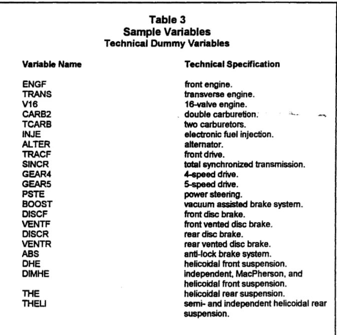
The data set has a large number cf charaderistics per sub-model (see table 3).

The data are composed cf numerical and dummy variables. The numerical variables

represent perfonnance and technical (physical) charaderistics. Dummy variables take

the value cf one if the particular sub-model possesses the charaderistic (as standard

equipment) and zero if it does not. The dummies variables are mostly related to

technicaVphysicaJ characteristics, though some dummies have been aeated to contrai the

sample.

As stated earlier, most models come in different sub-models. Some sub-models

differ by angine size, horsepower, or other components already incJuded among the

anywhere in the regression model. Therefore, I have introduced "Iuxury" dummy variables

to separate these sub-models. These variables (L 1, L2, and L3) allow me to account for

to up to four similar sub-models of a mode/. Wrthout these variables, some sub-models in our sample would differ only by price and market share.

Variable Name

ENGF TRANS V16

CARB2 TCARB

INJE

ALTER TRACF SINCR GEAR4 GEAR5 PSTE BOOST DISCF VENTF DISCR VENTR

ABS

DHE DIMHE

THE THEU

Table 3 Sample Variables

Technical Dummy Variables

Technical Specification

front engine. transverse engine. 16-valve engine. , double carburetion.

two carburetors. electronic fuel injection. altemator.

front drive.

total synchronized transmission. 4-speed drive.

5-speed drive. power steering.

vacuum assisted brake system. front disc brake.

front vented disc brake. rear disc brake.

rear vented disc brake. anti-Iock brake system. helicoidal front suspension. independent, MacPherson, and helicoidal front suspension. helicoidal rear suspension.

semi- and independent helicoidal rear suspension.

Variable Name SPEED ACCE DIST CONS C080 Variable Name CIlIN DISP HPS HPA LENG WBAS WEIG TANK TRUNK Variable Name AlCO GAS POPU l1,L2,l3 DOOR4 HATCH Table 3 Sample Variables Performance Variables Numerical Technical Specification top speed.

time to speed: 0-100 Kmlh. stopping distance: 80-0 KmIh. average tuel consumption.

fueI consumption at c:onsIantspeed (80 KmIh).

Technical Variables Numerical

Technical Specification

number of cylinders displacement horsepower horsepower length wheelbase weight tuel capacity trunk capacity

Dummy Contrai Variables

Unit KrnIh sec meter Km/J Km/J Unit unit cc continuation hp (SAE) hp (ABNT)

centimeter centimeter Kg liter liter Technical Specification fuel: ethanol. tuel: gasoline. ·popular" model. luxury leveis 1, 2, and 3. fourdoors.

•

Other control variables are DOOR4 to identify four-door models, POPU to

distinguish "popular" cars from the others, and ALCO and GAS to identify cars using

ethanol and gasoline, respectively, as fue!. "Popular" and cars with engine sizes under

1,000 cc carry significantly lower taxes. Thus, their prices are lower for reasons not

accounted for by their characteristics.11 Similarly, ethanol-fueled vehicles have a

lower price than their gasoline-fueled counterparts (also due to tax incentives), higher

fuel consumption, and, in general, higher horsepower.

4. The Regression Results

In spite of the theoretical questions about using the hedonic technique to

estimate quality change, diSOJSSed in section 2, some econometric specffication problems

must also be addressed by the researcher.12

A common problem one faces when estimating hedonic regressions is the

identification of the relevant set of characteristics. In the case of automobiles, for

example, the first dilemma is the choice between performance and physical

characteristics. When a consumerdecides to buy an automobile she is interested in the

performance cf the vehicle and not in its physical characteristics, per se. That is, she will be interested in the speed, handling, steering, driving position, comfort, etc. In

such case, the hedonicestimation should be based on performance variables because they

enter the utility function directly.

HoNever, most previous studies have been based on physical ratherthan performance

data. Two reasons for this are that physical information is more readily available and

that most perfoonance data is based on subjective conditions that may introduce a serious

measurement error.

The use of physical characteristics is justified by the assumption that

performance charaderistics are fundions cf physical charaderistics. As long as this

relationship does not change significantly, the use of physical characteristics as

proxies for performance d1aracteristics causes no probJem. lhis assumption may be

true

for the short run. However, most cf the innovation occurring in the car industry has

resulted in increased performance with little or no change in physical charaderistics.

For example, a new design may result in higher speed and acceleration rate. Using

horsepower to proxy for speed, without induding Itdesign" in the equation, would bias our results.

Otha and Griliches (1976) address this question and conclude that substituting

physical charaderistics for performance variables does not significantly affect the

tit, at least not for the short period from 1963 to 1966. In any case, I have combined

both kinds cf charaderistics. To avoid the bias introduced by subjective evaluations

I include just a few of the many performance variables available, the ones least

Another difficulty inherent in hedonic estimation is the omission of relevant

variables, which results in biased estimators.'3 _{For this study, an effort was made to}

build as complete a data set as possible. However, many pieces cf information available in one period cf time are not available in others. Additionally, information on some variables are not available for ali sub-models. Throughout 1 have faced a trade-off

belween the range of characteristics and sample size.

Multicollinearity is bound to be an issue in this kind cf study. Luxury models are higher quality, and 50 possess most of the quality charaderistics. Thus, one should

expect a high correlation among the variables in the sample. Two points should be made

here. First, of course it would be nice if the explanatory variables of a regression

"'

__ .

model were linearfy independent. However, to exclude variables with this gosl in mind

isto negatethe model'sfundamentals. As stated earfier, excluding variables may

aeate

specification problems, since one may be omitting a relevant variable. Additionally, it

is worth recalling that the least squares estimator will remain the best unbiased

estimator cf the parameters. As Greene points out (1993, p. 270), the problem with multicollinearity is that "best" is not very good.

Second, a consequence of multicollinearity is that the individual shadow

(implicit) price of a particular characteristic will not be well-identified. Although

multicollinearity affects the estimates of an individual variable's coefficient, it does

not affect their combined effect on prices. In this study, I am not particularly

the fitted path, that is, the effect of the whole set of characteristics (quality

variables) on price. Thus, with respect to the main purpose of this study,

multicollinearity is not a problem at ali.

A novelty presented in this analysis is the use of normalized variables. This

procedurehasbeen introducedtocompensateforthebiasc::reatedwhen comparingbig cars

with small ones. For example, as heavier cars need a longer distance to stop, I divided

DIST by WEIG (DISWEI). A similar rationaJe applies to horsepower: Cars with big engines

tend to have more horsepowerthan cars with small engines. To normalize the horsepower variable, I dMded HPS (ar HPA) by DISP (HPSCC ar HPACC).104 Note that this procecire also takes care cf the bias created by the V6 and V8 engines during the first

two

decades. Moreover, technically, HPS(A)CC is a better measurefor engine quality, namely, the power

per unit of displacement, that is horsepower per cubic centimeter.

WELENG (WEIG divided by LENG) is another norma/ized variable. lhe use ofthe weight variable has been justified as a proxyformore features, since a heaviercartends

to incorporate more features than a lighter one. On the other hand, its use has been

aiticized because, overtime the industry has reduce car weights (and lengths) without

reducing their quality. Smaller, Iighter cars with no significant loss in comfort

(intemal room) or performance have been introduced. Thus, the use of weight as an

explanatory variable should be pursued with caution.

Employing WELENG reduces the bias toward larga cars. However, the problem of

innovations that, other things equal, reduce car's weight remains. In summary, I have

replaced the usual set of physical characteristics: weight, length and horsepower by

WELENG and HPS(A)CC.

At last, it is worth to note that some variables may account for more than one

desired atbibute. For example, the variable TRANS, as well as being a proxy for a modem

engine, also ac:counts for internai space and modem design, because a transversa rather

than a longitudinal engine allows for more intemal room in a given

caro

The same is true

for DISWEI, which may account for both the quality of the brake system and for the

vehicle's stability.

"'L __

--In an attempt to improve the results of this study, I have decided to weight the

data. The rationale for this is that sometimes a manufacturer may set the ''wrong price,"

given the quality of its vehicle. Not accounting for such deviations from the "right

price" may bias our conclusions. To minimize the bias from mistakes and idiosyncrasies

in manufacturers' pricing policies, I have weighted the data by the mamet share cf each sub-model.15

Thus, the procedure used to estimate the hedonic equations was weighted least

squares, with mar1<et share as theweight. Weighted datawere computed by multiplying the original data by the square root cf the weights. The estimated coefficients are nothing

1~raphing the squared residuais (ofa non-weighted regresSon) against marketshare showed eWJence that observations with smaller marketshare tend to produce estimates with a higher deviation from the true price.

more than ordinary least squares coefficients forthe regression with weights. However,

the constant is no longer a constant, but is instead the square root of the weights.

Twogroupsofequations have been estimated, one based onthevariables SPEED and

VVELENG, aDthedherbasedCJ1Hps(A)CCa"d\NELENG. Thedatawere~

intfTee-year intervals, with the exception of the 1960s. Given the small number of observation during the 1960s, I opted for a four-year pooling (1960~3 and 1964~7).

The sample has been split according to the different phases in the industry's

development. This is an important issue: pooling different years is to assume that no

significant changes in consumers' taste or production costs occurred during the chosen

interval (refer to section 3 of this chapter).

"""--- ~

Thus, the first

two

periods are the industry's maturation phase. The "Miracle"

phase is split into

two

periods: 1968-70 and 1971-73. Intervals 1974-76 and 1977-79,

represent the "Retrenchment" phase. The 1980s were the era of the ethanol car and economicstagnation. Three intervals accountforthis phase: 1980-82, 1983-85, and

1986-88. lhe last phase, marked by trade liberalization, is represented by the periods 1989-91 and 1992-9418

•

I estimate equations for current prices, constant prices and US dollar prices.

As should be expected, the estimated coefficients have not been affected by changes on

price measurement. The use of different price series affects the "constanf' term, year-dummy coefficients, and the goodness of the fit, or more specifically, the R-squared statistic.

Given high inflation, especial/y during the last

two

decades, the use cf current

prices produces R-squared statistics very close to 1 (see table 4). The annual change in

prices is captured bythe year-dummies, and those changes

were

above 1 00 percent during

the 19aJs, and exceeded 2,CXXl percent in 1he 1990s. ftsl am interested in c:hanges on price due the charaderistics (quality) variables, it makes no difference which price series

is used.

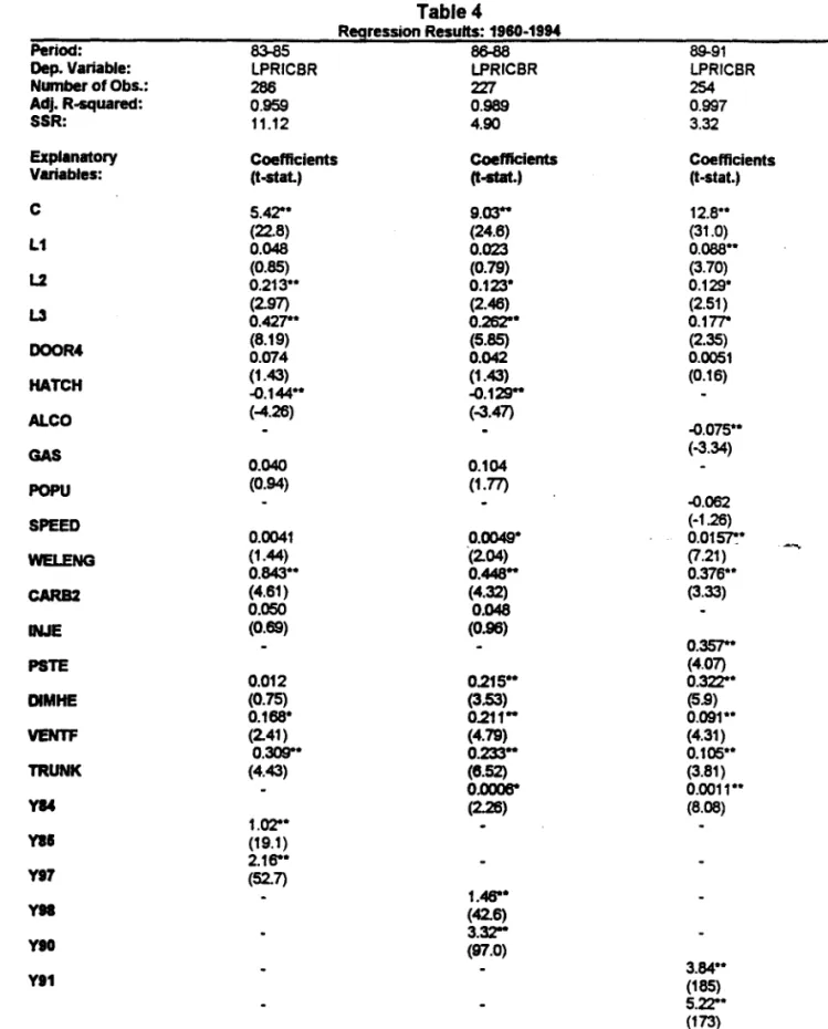
Tables 4 presents the results for group 1 (SPEED), using current prices. The tit

ofthese regessions is Vf!!4y good. 17 lhe CXIeffidents on SPEED and VVELENG are quite stable

and significantly different from zero from one equation to another. The notable

exception is the WELENG coefficient for the period 1983-85 that is well above the values

--forthe other periods. This behavior may reflect the fast growth rate in vehicles average

weight during the period (see tablas A. 1 and A.2). As will be discussed later, this probablymar1<s a shift in demandfrom small models to higher qualitymedium and

medium-larga models.

Table 4

R!!Iresslon Results: 1980-1994

Period: 60-63 64-67 68-70 71-73

Cep. Variable: LPRICBR LPRICBR LPRICBR LPRICBR

Number o'Obs.: 31 42 48 81

Adj. R-squared: 0.981 0.955 0.968 0.954

SSR: 0.112 0.250 0.112 .248

ExpIanatory Coeflicients Coefliclents Coefficients Coeflicients

Variables: _(t-stat» (t-stat, (teStat.) (t-stat»

C -2.10** -O.56Er 0.968" 1.11**

Li 0.210-(-3.33) 0.093 (-2.11) 0.135" (5.85) (9.16) 0.065*·

L2 (5.85) _-0.020 (1.24) (5.06) (2.00) _0.190'

DOOR4 (-0.41) _{-0.020 0.024} (2.64)

SPEED _{0.0082 0.0096'"} (-0.49) _0.0061*' (0.73) _0.0072"

WELENG (1.22) _0.342*' (2.85) _0.405** (4.06) _0.319'* (5.43) _0.345"

CARB2 (4.14) _0.139 (4.35) _0.089 (10.8) _0.011 (3.93)

0.023

PSTE (0.97) (1.56) (0.27) (0.48)

0.111 0.267** 0.196*'"

DHE (1.62) (6.20) (3.98)

0.0003 -0.195' 0.051 0.082"

DISCF (0.006) (-2.23) (1.71) (2.86)

0.099 ~O.O87*· _ .,

BOOST (1.73) (3.06)

0.054

Vii (1.90)

0.205"

VI2 (4.32) 0.426"*

VI3 (9.10)

1.12"

VII (28.4)

0.383·*

VII (5.24)

0.567"*

VI7 (7.59)

0.746**

VI' (9.06)

0.153"

Y70 (6.14)

0.255'*

Y72 (8.26)

0.107**

Y73 (3.79)

0.171** {6.16l • Significant at 95 percent. .* Slgnificant at 99 percent. t-statistics are in parentheses.

Table 4

R!,gression Results: 1980-1994

Period: 74-76 n-79 80-82

Cep. VariabJe: LPRICBR LPRICBR LPRICBR

Number of Obs.: 132 154 263

AdJ. R-equared: 0.973 0.971 0.981

SSR: 0.363 0.629 2.71

EzpIanatory _{Coeflic:ients Coefficients Coefficients}

VariabIes: _{(t-stat.) (t-stat.) (t-stat)}

C _{2.00-* 248** 3.54**}

L1 (15.3) _.0.65** (17.6) _0.063** (22.0) _0.089**

L2 _0.014 (3.71) _0.103** (2.80) (5.01) _0.131**

L3 (0.78) (3.00) (281) _0.260**

DOOR4 _{0.055* 0.049 0.064} (7.32)

HATCH (222) _0.0010 (1.37) _-0.039 (1.55)

-0.073*

ALCO (0.04) (-0.17) (-232)

-0.033

SPEED (-1.72)

0.0045** 0.0031 0.0025*

WELENG (3.08) (1.59) (255)

0.234- 0.503- 0.659**

CARB2 (4.66) (4.55) (6.10)

0.071* 0.147"* 0.084-· --.

PSTE (200) (4.31) (2.87)

0.369** 0.139 0.199**

DItE (9.02) (1.45) (2.87)

0.123** 0.072

DlMHE (4.96) (1.97)

0.11'-DlSCF (4.15)

0.071**

BOOST (3.22)

0.074** 0.153** 0.170**

VENTF (3.37) (4.95) (6.51)

0.014

Y71 (0.41)

0.327**

Y7. (16.4)

0.539**

Y78 (30.2)

0.317**

Y7I (12.2)

0.732**

Vl1 _(27.6)

YI2 0.816** _(50.2)

1.64**

~87.11

* Slgnificant at 95 percent. ** Significant at 99 percent. t-statistics are in parentheaes.

Table4

R!:gression Results: 1960-1994

Period: 83-85 86-88 89-91

Cep. Variable: LPRICBR LPRICBR LPRICBR

Number of Obs.: 286 2ZT 254

Adj. R-squared: 0.959 0.989 0.997

SSR: 11.12 4.90 3.32

Explanatory _{Coefficients Coefficients Coeflicients}

Variables: _(t-stat.) (t-stat.) (t-stat.)

C 5.42*- 9.03"

12.8--L1 (22.8) _0.048 (24.6) _0.023 (31.0) _0.088" L2 _0.213--(0.85) (0.79) _0.123- (3.70)

0.129-L3 _0.42~-(2.97) _0.262"-(2.46) _0.17r (2.51)

DOOR4 _0.074 (8.19) (5.85) _{0.042 0.0051} (2.35)

HATCH (1.43) _{-0.144-- -o.12r} (1.43) (0.16)

ALCO (-4.26) (-3.47)

-0.075--GAS (-3.34)

0.040 0.104

POPU (0.94) (1.77)

-0.062

SPEED (-1.26)

0.0041 0.0049- 0.01sr _~

...

WELENG (1.44) '(2.04) (7.21)

0.843-- 0.448"

0.376--CARB2 (4.61) (4.32) (3.33)

0.050 0.048

INJE (0.69) (0.96)

o.~

PSTE (4.07)

0.012 0.215--

0.322*-DlMHE (0.75) (3.53) (5.9)

0.168- 0.211"

0.091--VENTF (2.41 ) (4.79) (4.31)

0.309-- 0.233"

0.1OS--TRUNK (4.43) (8.52) (3.81)

o.oooe-

0.001'--YI4 (2.26) (8.08)

1.02*-VI'

(19.1 )

2.16"-VI7 (52.7)

1.46"-VII (42.6)

3.3r

VIO (97.0)

3.84--VI1 (185)

5.22*-~173l

- Slgnificant aí 95 percent. --Significant at 99 percent. t-etatistics are in parentheses.

Table4

Regression Results: 1980.19114

Period: 92·94

Cep. Variable: lPRICBR

Number of Obs.: 185

AdJ. R-squared: 0.999

SSR: 1.57

Explanatory Coefficients

Variables: (t-stat.)

C _22.9"

Li (64.3) 0.061

l2 _0.256"· (1.68)

DOeR. (7.32) _0.025

ALCO (0.65) _-0.0002

POPU (-0.007) _-0.3230

•

SPEED (~.79)

0.0025

WELENG (1.40)

0.372"

INJE (3.29)

0.093··

PSTE (2.83)

0.31400

VENTF (5.95)

0.1530 •

A8S (2.71)

0.2280 •

TRUNK (3.95)

0.0007*·

YI7 (3.17)

VII no

VIi

VIS

2.900 •

YM (76.7)

6.56" (147)

o Slgnificant at 95 percent. "SlgniflCant at 99 percent. t·&tatistics are in parentheses.

Vou may note that SPEED and WElENG are the only variables that appears in ali

estimations. The set of the remained variables changes over time according to their

quality relevance. For example, double carburetion was a major innovation until1989,

when it was replaced by electronic fuel injection. Thus, starting in 1989, the relevant

variablebecomes INJE instead of CARB2. Othervariables, as frontdisc brake(DISCF) and vacuum-assisted brakesystem (BOOST), forexample, become standard duringthe period,

losing its relevance to the analysis (see tables A.1 and A.2).

lhe estimated c:oefficients give us the percentage change in price associated with

a change on the relevant characteristic. For example, in 198Q..82, a one KmIh inaease in theaveragetop speed ofBrazilian-made passengercarsWouId result in an inaease ofO.25

percent in the average price. The same estimation suggests that the introdudion of

vacuum-assisted brake system would increase the average price by 17 percent. 18

The quality change index was built by multiplying the charaderistics' change in

the period by their estimated coefficients, and adding them up. The result gives us the

percentage change in price attributable to quality changes. Thus, assuming 1980 as the

base

year

(1980=1 (0), the weighted index value for 1981 was c:onstruc:ted as follows: The

quality change from 1980 to 1981 is (0.0025 x 3) + (0.659 x -0.002) + (0.084 x 0.025) +

(0.199 x -0.001) + (0.111 x 0.048) + (0.17 x 0.194) + (0.014 x O.O)

=

0.046. Thus, the index for 1981 is 104.6.

'9

18As stated earlier, beca use of multicollinearity, this interpretation should be taken with caution.

Figures 2 depids the quality change index for specification 1 (SPEED) and 2

(HPCC), based onthe non-weighted sample (Ieft graph) and theweighted one (right graph). Note that changing specification barely affects our results, except when comparing. a

series over a brief period of time.

Figure 2a

Quality Change Indexes

Brazman AutornobiIe 1ndus1ry Nan-Wllighlad Sampla

lGt10 - 1904

200~---~

180 ... . 180

140 120 100 80

~-80 ,~98O+++,+-4966.-t+t~,9~70+++,9t175~,~980+++,+-1966~ ... ,990+++++I

- Equation 1 (SPEED) - Equation 2 (HPIDISP)

Figure 2b

Quality Change Indexes

Brazilian Automobile lnc1Jstry

W8Ighlad Sampla 1Q60 - 1;94

180 -r---,~ 180 140 120 100

8Ot...~~

8O+H~~~~~~~*H~~

1980 1965 1970 1975 1980 1985 1990

- Equation 1 (SPEEDt- Equation 2 (HPIDISP)

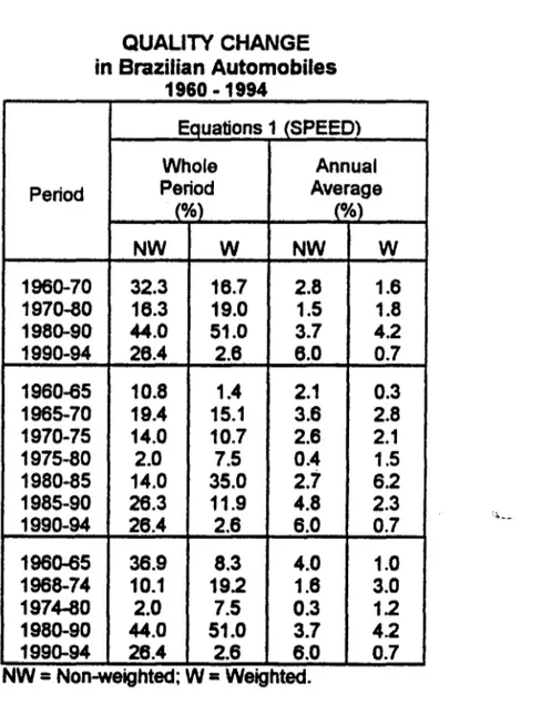
A summary of the quality change in Brazilian automobile is presented in the

following table. Table 5 shows the change in automobile quality (equations 1) for

TABLE 5

QUALlTY CHANGE

in Brazilian Automobiles 1960 -1994

Equations 1 (SPEED)

Whole Annual Period Period Average

(%) (%)

NW W NW W

1960-70 32.3 16.7 2.8 1.6 1970-80 16.3 19.0 1.5 1.8 1980-90 44.0 51.0 3.7 4.2 1990-94 26.4 2.6 6.0 0.7

1960-65 10.8 1.4 2.1 0.3 1965-70 19.4 15.1 3.6 2.8 1970-75 14.0 10.7 2.6 2.1 1975-80 2.0 7.5 0.4 1.5 1980-85 14.0 35.0 2.7 6.2 1985-90 26.3 11.9 4.8 2.3 1990-94 26.4 2.6 6.0 0.7

1960-65 36.9 8.3 4.0 1.0 1968-74 10.1 192 1.6 3.0 1974-80 2.0 7.5 0.3 12 1980-90 44.0 51.0 3.7 4.2 1990-94 26.4 2.6 6.0 0.7 NW

=

Non-welQhted: W

=

WelQhted.

Figure 3 compares the quality change index for the non-weighted and weighted

samples, specification 1 (SPEED). Note that the index based on the non-weighted sample iIIustrates quality change in the automobile supply, while the index based on the

weighted sample yields the quality evolution cf the average domesticaJJy-produced car

sold in the Brazilian market. The distinction is important. It aJlow us to identify

quality changedriven bychanges in demand versus those driven by supply-sidefadors.

For example, a significantly higher rate of change in the weighted index suggests a shift

Figure 3

Quality Change Indexes

Brazilian Automobile Industry

Equation 1 (SPEED)

1960 - 1994

200~---~

180+---~

160+---~.-~~

140+---~--~--~

120+---~_,~----~

100r---~~~~~~---_1

~~~~~---I

OO~~~HH~~~~~++~~~~~~

1960 1965 1970 1975 1980 1985 1990

- Non-Weighted Index - Weighted Index

As can be see on figures 2 and 3, and table 5, the quality of Brazilian=-made passenger cars grew steadily for almost ali cf the first two decades of the industry's existence. It is interesting that the enormous rate of growth of output during 1968-74

(see figure 1), apparently had little effect on the rate of quality change.

After 1980, the numbers change dramatically. While the Brazilian economy, and

consequently, the automobile industryfaced a big recession, the quality of automobiles

increased at a rate without precedent. Comparing the non-weighted series with the

weighted one reveals

two

major dlanges. During the first half cf the 1980s, the weighted index rose by 35 percent, compared to a rise cf 14 percent in the non-weighted index. This

reflects a shift in demand toward cars cf higher quality. 111e opposite happened in the 1990s. From 1990to 1994, the non-weighted indexgrewby26.4 percentwhiletheweighted

index rose by only 2.6 percent, reflecting a shift in demand for domestic automobiles

toward lower quality models20 .

A comparíson cfthese results with similar estimates for the U.S. automobile

market shows that, from 1960 to 1985, the quality ofthe average Brazilian-made car has

improved proportionally more than the quality of the average car sold in America (see

table 6).

Table 6 presents estimates cf quality change for U.S. automobiles. However, these qua/ity change indexes are cf no use if we want to compare the quality of an average

Brazilian car with an average American caro 111e on/y comparison possib/e is of the quality evolution in the

two

markets, that is, the proportional change in car quality.

;J. __

111e index says nothing about absolute qua/ity. Moreover, the reduction in vehicJe size

during the 19705 and 19805, was much more marked in the U.S. than in Brazi!. Historically, the average size cf cars so/d in the U.S. was much bigger than that of cars

so/d in Brazi!. As length and weight are primary characteristics used in these

regressions, we should expect a smaller rate of change in the U.S. during this período

Also, one should acknowledge that most product innovation in Brazil's auto

industry has consisted cf adopting

new

technology already used in other countries. Thus

higher rate cf change, instead cf indicatíng better quality cars, may be a signal cf lower

quality at the beginning of the período The lower the initial qua/ity, the bigger will

be the proportional change needed to bring quality doser to the state-of-the-art.

TABLE6

Quality Change in U.S. Automobiles

Domestic Cars

Rate of Change (%)

Period Source

Total Average

1906-14 87.4 17.0 Raff and Trajtenberg

1914-24 -4.9 -1.0 (1995)

1924-32 57.4 12.0

1930-40 -44.2 -11.0

1937-50 22.7 1.6 Griliches (1961)a

1950-54 2.2 0.5

1954-60 20.0 3.1

1954-60 16.1 2.5

1960-68 -8.0 -1.2 Triplett (1969)

1947-50 -7.4 -2.5 Gordon (1990)b

1950-55 14.1 2.7

1955-60 11.6 2.2

1960-65 -10.1 -2.1

::,ç.--1965-70 5.4 1.1 ~

...

1970-75 5.1 1.0

1975-80 -8.1 -1.7

1980-83 -1.6 -0.5

1979-84 5.6 1.1 Feenstra (1985t

Japanese Imported Cars

1979-85 27.1 3.5 Feenstra (1985)C

a. Row 1 and 3: adjacent years; row 2 and 4: pooling 1954-80.

b. Values calculated deducting the change in the average stripped price (Tb. 8.3) from th change in the hedonic index (Tb. 8.8).

c. Small cars.

Despite ali these considerations, the speed of quaJity change in Brazilian

automobiles after 1980, is still impressive. The U.S. industry on/y achieved higher

their largest contributions to society.21 This shows that it is not difficult for an

industry consisting of transnational firms to bring its product to the state-of-the-art

leveI. It just needs the right incentives.

The hedonic technique can also be used to estimate the process innovation effec:t.

One may decompose a price change into

two

components: produd and process innovation

related. The quality change index estimated here identifies the change in prices due to

produd innovation. The residual change, that is, the change in the quality-adjusted

price, may be considered an effect of process innovation. However, as Raff and

Trajtenberg (1995) wam, this decomposition should be undertaken cautious/y. Prices can change due to many other fadors, such as, changes in input price or in the degree of

~

c:ompetition in the market Moreover, some produdivity gains may not be passed

âiõng

to prices, and so will not be captured by price movements.

Figure 4 presents the real weighted average price of passenger cars, excluding station wagons. The prices have been deftated by the wholesale price indax (IPA-DI) and

are measured in auzeiros of November-December cf 1963. The figure depids two series of real prices, one not adjusted for and the other adjusted for quality.

The unadjusted real weighted average price fell from 2,980 to 1 ,445 auzeiros

between 1960 and 1980. During the 1980s, it inaeased by more than 90 percent, reaching its peak value cf 2,758 in 1988. The unadjusted real weighted average price then fell again and practically stabilized a fittle above 2,000 auzeiros. On the other hand, the quafity-adjusted price kept falfing, though not without interruption, until 1986. After

reaching a low cf 840 cruzeiros, the adjusted average price became quite stable

at

the 950 cruzeiros levei (see table A.5).

Figure 4

Weighted Average Real Price

Brazilian Passenger Cars

1960 -1994

3,000 ___ - - - ,

2,500 ... ~""'"l---++_-~

2,000 +----~.;ap. ___ -__.. _ _+---~~

1,500

+---+_-""'---1

1,000

+---...

~_:___f~=__:A-f

Prices in 1963 Cr$ waighted by market shara.

500~+H~~~~~~~~+HH+~~

1960 1965 1970 1975 1980 1985 1990

- Non Adjusted Price - Quality Adjusted Price

Ifwe assume that a price change, holding produd quality constant, is a result of

process

innovation,

we

can build an index of

process

innovation passed on to consumers.

Figure 522 _{compares such an index with labor produdivity in the automotive industry. It}

is clear that the

two

series foUow a very similar path during the first

two

decades. The

correlation coefficientfor the 1960-79 period is .955, but faUs to .672 when calculated

By the end of the 1970s, as labor productivity stopped rising, the process

innovation index starts to f1uduate wildly. As this index is calculated as a residual,

the higher variance for the 1980s and 1990s is probably a result of very high inflation.

In this case, quality-adjusted prices would be changing for reasons other than changes

in productivity, such as unfulfilled inflation expectations.

lhe comparison between the process innovation index and labor produdivity is

evidence that, during periods of lower inflation (or at least not extremely high

inflation), changes in quality-adjusted real price was driven mostly by changes in

productivity.

Figure 5

Process Innovation Index

and Labor Productivity

Brazillan Automotive Industry

16~---T~

Vehicles per 14 employees.

12

10 8 6 4

1960-1994

250

200

150

2 100

1960 1965 1970 1975 1980 1985 1990

5. Conclusion

The ma in target of this work was to build a quality change index for the Brazilian

automobile industry. To the best of my knowledge, this is the first time such index has

been constructed. Moreover, as important as the estimation of the index was the

construction cf the data set for the Brazilian passenger cars. The data set comprise

information on attributes, prices, and volume of sales for the period 1960-1994.

The estimation cf a quality change index for the Brazil's auto industry has two

major significance. They allow a better understanding cf produd innovation in Brazil's

auto industry, as well as a better understanding of the behavior of auto prices.

;'t.__ .--,.

For example, it has been shown that the real average price, when adjusted for

changes in quality, has fallen more than commonly supposed. Moreover, duringthe 1980s and 1990s, most cfthe real price inaease was due

to

an inaease in vehide quality. The

quality-adjusted real average price, pradically remained constant. Interesting too,

is the suggestion that trade liberalization had no apparent effect on prices.

In the matter cf product innovation, the index show us that the "Iost decade," as

the 1980s have been known, was, in fad, a period of significant evolution in the quality

cf the Brazilian-made automobiles. Additionally, the index construded here allows us

Reference

ANFAVEA(1995), StatisticalYearbook, TheBrazi5anAutomotivelndustry: 1957-1994, São Paulo: Associação Nacional dos Fabricantes de Veículos Automotores.

Bemdt, E.R. (1990), '111e Measurement cf Quality Change: Construding an hedonic price index for computers using multi pie regression methods," in Bemdt, E.R., The

Pradice ofEconornetrt:s: CIassic and Contemporary, Reading, MA: Addison-Wesley,

pp. 102-149.

Court, A T. (1939), ''Hedonic Price Indexes with Automotive Examples," in Ihe Dynamicsof

Automobile Demand, New York: The General Motors Corporation, pp. 99-117

Epple, D. (1987), "Hedonic Prices and Implicit Markets: Estimating Demand and Supply Functions for Differentiated Products," Journal of Political Economy, 95, February, pp. 59-80.

Feenstra, R.C. (1987), "Voluntary export restraint in U.S. autos, 1980-81: Quality, employment, and Welfare effects," in Bhagwati, J.N. (ed.), Intemational Trade:

selected readings, Cambridge: MIT Press, pp. 203-30.

'"-~ ....

Feenstra, R.C. (1988), "Quality change under trade restraints in Japanese autos,"

Quarter/y Journal of Economics, February, pp. 131-146.

Ferro, J.R. (1994), liA Indústria automobilística no Brasil: desempenho, estratégias e opcões de política industrial," mimeo.

Fonseca, R (1996), "Produd Innovation in Brazilian Autos," Ph.D. Dissertation, U.C. Berkeley, Department of Economics.

Gordon, RJ. (19a»), TheMeasuremenfofDurableGoodsPrms, NBERMonograph, Chicago: University of Chicago Press.

Greene, W.H. (1993), Econometric Analysis, 2nd _{Edition, New York: Macmillan.}

Griliches, Z. (1961), "Hedonic price indexes for automobiles: an econometric analysis of quality change," The Price statistics of the Federal Government (General Series, No. 73), NewYork: National Bureau ofEconomic Research. Reprinted in Griliches, Z. (ed.), Price Indexes and Quality Change: Studies in new methods of

Griliches, Z. (1971), "Introduction: Hedonic Price Indexes Revisited," in Griliches, Z. (ed.), Price Indexes and Quality Change: Studies in new methods of measurement,

Cambridge: Harvard University Press, 1971.

Griliches,

Z.

(1990), "Hedonic Price Indexes and the Measurement of Capital and Productivity: Some Historical Reflections," in E.R. Bemdt and J.E. Triplett, FiIty Years of

Eax70rnC

Measurement: The Jubüee dthe Conference on Research

in

Income and Wealth, Chicago: University cf Chicago Press.

Lancaster,

K

(1971 ), ConsumerDemand: a newapproach, New

York:

Columbia University Press.

McFadden, D. (1981), "EconometricModelsofProbabilisticChoice," inC.Manskiand

D.

McFadden (eds.), Strucfural Analysis of Discrete Data with Econometric Applications. Cambridge: MIT Press.

Ohta, M. andZ. Grilid1es (1976), "Automobile Prices Revisited: Extensions ofthe Hedonic Hypothesis,"in Terleckyj, N.E. (ed.), HouseholdProductionandConsumption, NBER

Studies in Income and Wealth, vol. 40, New York: Columbia University Press,

pp.325-390. "-__ -.

Ohta, M. and Z. Griliches (1986), "Automobile Prices and Quality: Did the gasoline price

increases

change

consumer tastes

in

lhe

U.S.?," Joumal of Busness & Economic Statistics, April, vol. 4, no. 2, pp. 187-198.

Payson, S. (1994), Quafrty Measurementin Econornics: New Perspectiveson theevolution of goods and services, Hants, U.K: Edward Elgar.

Raff, D.M.G and M. Trajtenberg (1995), "Quality-Adjusted Prices for the American Automobile Industry: 1906-1940," NBER Working Paper No. 5035, February.

Rosen, S. (1974), "Hedonic Prices and Implicit Markets: Product Differentiation in Pure Competition," Journal of Polítical Economy, 82, January-February, pp. 34-55.

Train, K (1986), Qualitativa Choice Analysis: Theory, Econometrics, and an App/ication

to Aufomobile Demand, Cambridge: The MIT Press.

Trajtenberg, M. (1990), EconornicAna/ysisofProductlnnovation: The CaseofCTScanners,

Cambridge: Harvard University Press.

Triplett, J.E. (1990), "Hedonic Methods in Statistical Agency Environments: Arl intellectual biopsy," in

E.R.

Bemdt and J.E. Triplett, Fifty Years of Economic Measurement: The Jubilee ofthe Conference on Research in Income and Wealth,

Chicago: University of Chicago Press.

Womack, J.P., D.T. Jones, andO. Ross(1990), TheMachinethatChangecJthe World, New

YEAR LENG

Cm 1960 442 1961 446 1962 450 1963 448

1964 445 1965 445 1966 450 1967 451 1968 458 1969 459 1970 454 1971 459 1972 456 1973 453

1974 452 1975 451 1976 449 19n 450

1978 446

1979 447 1980 438 1981 435 1982 430 1983 423 1984 422 1985 426 1986 427 1987 429 1988 432 1989 426 1990 426 1991 426 1992 418 1993 422 1994 419 1990 426 1991 427 1992 421 1993 425 1994 424 1990 364

1991 364

1992 382 1993 383 1994 380

TABLE A.1

Characteristics of Brazilian Passenger Cars (excl. S.W.)

WBAS Cm 255 257 258 256 255 255 258 258 263 263 260 262 260 259 260 259 259 259 258 257 252 251 247 245 246 247 248 249 249 249 250 250 246 250 251 250 250 247 251 252 236 236 237 237 238

on- elal ted am~e: 1

-N W' h S I 960 1994

Averaae

WEIG TANK TRUNK DISP HPS HPA

Kg liter liter cc hp (SAE) hp (ABNT)

1.044 n.a. n.a. 1.664 69 n.a. 1.071 n.a. n.a. 1762 72 n.a. 1,110 n.a. n.a. 1835 78 n.a. 1092 n.a. n.a. 1,794 79 n.a. 1126 n.a. n.a. 1,756 78 ·n.a. 1,126 n.a. n.a. 1,756 79 n.a. 1,172 n.a. n.a. 1888 90 n.a.

1155 n.a. n.a. 1981 93 n.a.

1223 n.a. n.a. 2282 103 n.a. 1.173 n.a. n.a. 2439 103 n.a. 1120 n.a. n.a. 2453 101 n.a. 1,158 n.a. n.a. 2807 112 n.a. 1133 n.a. n.a. 2858 113 n.a. 1142 n.a. n.a. 2862 114 n.a. 1143 n.a. n.a. 2826 114 n.a. 1128 n.a. n.a. 2654 109 n.a. 1114 n.a. n.a. 2.562 110 n.a. 1129 n.a. n.a. 2,480 10T- _lt.a. 1123 n.a. n.a. 2,392 105 n.a.

1132 61 n.a. 2480 108 n.a.

1066 59 n.a. 2-,-194 96 n.a.

1047 59 n.a. 2.072 94 n.a.

1002 56 n.8. 1,733 85 71

966 59 n.a. 1,669 86 72

974 60 n.a. 1700 n.8. 76

1008 62 n.8. 1851 n.8. 83

1032 63 360 1887 n.a. 87

1038 62 370 1925 n.a. 90

1.041 66 363 1901 n.8. 89

1036 63 343 1913 n.a. 92

1,036 62 336 1901 n.a. 93

1033 60 337 1923 n.8. 94

1029 59 325 1.n9 n.a. 92

1073 60 335 1801 n.8. 96

1067 61 329 1,n1 n.8. 98

c Ing 'opu es

~ 100 .p lar" Mod 1

1,038 62 338 1910 n.8. 93

1036 60 338 1936 n.8. 95

1041 59 332 1835 n.8. 95

1094 61 345 1868 n.a. 100

1096 63 344 1859 n.8. 104

·POPular" Models

820 55 224 994 n.8. 48

820 50 224 994 n.8. 48

852 51 215 996 n.a. 49

855 51 229 1096 n.8. 55

842 48 213 1080 n.8. 54

TABLE A.1

Characteristics of Brazllian Passenger Cars (excl. S.W.) N on- elql t W' h ed S ample: I 1960 1994

-AveraQa

YEAR WBLENG WELENG HPSCC HPACC DISWEI Kg/Cm hplcc hp/cc meter/KQ

1960 0.5763 2.330 0.0414 n.a. 0.0274 1961 0.5748 2.368 0.0410 n.a. 0.0269 1962 0.5738 2.437 0.0422 n.a. 0.0263 1963 0.5722 2.411 0.0438 n.a. 0.0270 1964 0.5729 2.495 0.0442 n.a. 0.0257 1965 0.5729 2.495 0.0454 n.a. 0.0257 1966 0.5723 2.567 0.0473 n.a. 0.0251 1967 0.5714 2.517 0.0478 n.8. 0.0274 1968 0.5749 2.626 0.0453 n.a. 0.0264 1969 0.5729 2.526 0.0434 n.8. 0.0285 1970 0.5719 2.430 0.0433 n.a. 0.0262 1971 0.5716 2.493 0.0420 n.8. 0.0256 1972 0.5717 2.459 0.0417 n.a. 0.0263 1973 0.5733 2.497 0.0420 n.a. 0.0259 1974 0.5757 2.501 0.0425 n.a. 0.0270 1975 0.5763 2.478 0.0431 n.a. 0.0280 1976 0.5no 2.452 0.0453 n.a. 0.0291 19n 0.5no 2.480 0.0457 n.a. 0.02n

-1978 0.5794 2.490 0.0462 n.a. 0.0290 1979 0.57n 2.499 0.0458 n.a. 0.0303 1980 0.5783 2.404 0.0454 n.a. 0.0336 1981 0.5n3 2.3n 0.0469 n.a. 0.0338 1982 0.5765 2.314 0.0500 0.0421 0.0345 1983 0.5789 2.275 0.0521 0.0438 0.0354 1984 0.5850 2.301 n.8. 0.0455 0.0345 1985 0.5823 2.354 n.a. 0.0463 0.0331 1986 0.5825 2.404 n.8. 0.0478 0.0320 1987 0.5818 2.411 n.8. 0.0488 0.0310 1988 0.5784 2.403 n.8. 0.0482 0.0308 1989 0.5864 2.427 n.8. 0.0497 0.0301 1990 0.5889 2.427 n.8. 0.0499 0.0299 1991 0.5884 2.418 n.8. 0.0501 0.0300 1992 0.5912 2.453 n.8. 0.0514 0.0313 1993 0.5953 2.537 n.a. 0.0530 0.0291 1994 0.6009 2.538 n.8. 0.0548 0.0291

ExcludinQ ·PoPular" Models

1990 0.5883 2.4293 n.8. 0.0500 0.0298 1991 0.5875 2.4201 n.a. 0.0502 0.0299 1992 0.5889 2.4692 n.a. 0.0515 0.0308 1993 0.5928 2.5651 n.a. 0.0533 0.0283 1994 0.5973 2.5781 n.a . 0.0553 0.0280

loPU e

• p lar" Mod Is

TABLE A.i

Characteristlcs ot Brazillan Passenger Cars (excl. S.W.) on- e.gl ample:

-N W· hted 5 I 1960 1994

Average Pro ~ortion of new cars wlth YEAR SPEED ACCE DIST DOOR4 ENGF TRACF TRANS

Knv'h sec meter % % % %

1960 126 30.3 26.2 83.3 66.7 16.7 0.0

1961 127 29.5 26.7 85.7 71.4 14.3 0.0

1962 128 29.2 27.1 87.5 75.0 12.5 0.0

1963 127 29.2 27.9 90.0 70.0 10.0 0.0

1964 127 27.0 26.7 88.9 66.7 11.1 0.0

1965 128 25.2 26.9 88.9 66.7 11.1 0.0

1966 137 23.7 27.4 90.9 72.7 9.1 0.0

1967 138 23.7 29.4 84.6 69.2 15.4 0.0

1968 142 22.0 29.9

n.8

66.7 0.0 0.0

1969 144 20.1 31.7 78.9 84.2 21.1 0.0

1970 144 19.8 27.6 65.0 75.0 25.0 0.0

1971 150 17.6 27.9 60.0 80.0 20.0 0.0

1972 152 17.6 28.3 41.7 75.0 20.8 0.0

1973 150 18.4 28.2 31.3 78.1 15.6 0.0

1974 150 17.3 29.4 33.3 82.1 17.9 0.0

1975 149 17.8 29.9 35.4 . 81.3 18.8 0.0

1976 151 17.5 30.6 35.6 88.9 28.9 0.0

19n 147 17.3 29.5 38.0 92.0 28.0 -- 2:'0

1978 150 17.6 30.7 32.0 92.0 30.0 6.0

1979 148 18.2 32.0 35.2 88.9 25.9 7.4

1980 145 19.1 34.0 30.7 88.6 40.9 8.0

1981 145 18.8 33.8 33.3 . 89.6 47.9 7.3

1982 145 18.8 33.4 27.8 92.4 60.8 13.9

1983 149 17.0 33.6 35.0 98.1 76.7 27.2

1984 152 15.8 33.0 35.6 99.0 n.2 39.6

1985 154 15.3 32.6 30.1 98.8 78.3 37.3

1986 157 14.5 32.2 29.7 98.6 75.7 33.8

1987 155 13.9 31.7 29.2 100.0 80.6 43.1

1988 157 13.7 31.6 35.7 100.0 n.4 36.9

1989 159 13.0 30.7 34.9 100.0 84.9 50.0

1990 160 12.5 30.5 29.9 100.0 87.6 51.5

1991 160 12.6 30.5 30.7 100.0 88.0 58.7

1992 164 13.5 31.6 25.0 100.0 95.0 68.3

1993 169 13.3 30.4 29.0 100.0 98.6 63.8

1994 173 12.9 30.2 32.3 98.4 98.4 66.1

c Ing 'opu e

~ 100 • P lar" Mod Is

1990 160 12.4 30.5 30.2 100.0 87.5 51.0

1991 160 12.5 30.5 31.1 100.0 87.8 58.1

1992 166 12.8 31.5 26.8 100.0 96.4 69.6

1993 171 12.7 30.2 30.2 100.0 100.0 63.5

1994

1n

12.4 30.0 32.7 100.0 100.0 65.5

·Popular" Models

1990 136 20.0 31.2 0.0 100.0 100.0 100.0

1991 136 20.0 31.2 0.0 100.0 100.0 100.0

1992 133 23.5 32.5 0.0 100.0 75.0 50.0

TABLE A.1

Characteristics 01 BraziJIan Passenger Cars (excl. S.W.)

an- elai ample:

-N W I hted S I 1960 1994

Pro i)ortion 01 new cars with

YEAR CARB2 TCARB INJE AlTE SINCR PSTE BOOST DISCF

% % % % % % % %

1960 33.3 0.0 0.0 0.0 33.3 0.0 0.0 0.0

1961 42.9 0.0 0.0 0.0 42.9 0.0 0.0 0.0

1962 50.0 0.0 0.0 0.0 37.5 0.0 0.0 0.0

1963 50.0 10.0 0.0 0.0 70.0 0.0 0.0 0.0

1964 33.3 22.2 0.0 0.0 66.7 0.0 0.0 . 0.0

1965 33.3 22.2 0.0 0.0 n.8 0.0 0.0 0.0

1966 45.5 18.2 0.0 63.6 81.8 0.0 0.0 0.0

1967 46.2 7.7 0.0 76.9 84.6 7.7 0.0 0.0

1968 55.6 11.1 0.0 66.7 88.9 11.1 0.0 0.0

1969 36.8 5.3 0.0 84.2 100.0 10.5 0.0 5.3

1970 30.0 15.0 0.0 100.0 100.0 10.0 10.0 20.0 1971 32.0 16.0 0.0 100.0 100.0 12.0 12.0 24.0 1972 29.2 16.7 0.0 100.0 100.0 12.5 20.8 70.8 1973 28.1 12.5 0.0 100.0 100.0 9.4 21.9 68.8 1974 28.2 10.3 0.0 100.0 100.0 7.7 30.8 82.1 1975 41.7 10.4 0.0 100.0 100:0 6.3 33.3 85.4 1976 48.9 4.4 0.0 100.0 100.0 8.9 53.3 95.6

19n 54.0 6.0 0.0 100.0 100.0 8.0 54.0- ""96.0 1978 54.0 6.0 0.0 100.0 100.0 8.0 60.0 96.0 1979 59.3 7.4 0.0 100.0 100.0 11.1 50.0 96.3 1980 47.7 11.4 0.0 100.0 100.0 15.9 58.0 95.5 1981 46.9 12.5 0.0 100.0 100.0 15.6 64.6 95.8 1982 46.8 11.4 0.0 100.0 100.0 10.1 78.5 94.9 1983 61.2 5.8 0.0 100.0 100.0 5.8 89.3 98.1 1984 63.4 5.0 0.0 100.0 100.0 5.9 89.1 100.0 1985 60.2 3.6 0.0 100.0 100.0 7.2 91.6 100.0 1986 71.6 4.1 0.0 100.0 100.0 10.8 90.5 100.0 1987 81.9 0.0 0.0 100.0 100.0 11.1 94.4 100.0 1988 78.6 0.0 0.0 100.0 100.0 19.0 100.0 100.0 1989 86.0 0.0 1.2 100.0 100.0 19.8 100.0 100.0 1990 83.5 0.0 4.1 100.0 100.0 22.7 100.0 100.0 1991 80.0 0.0 5.3 100.0 100.0 24.0 100.0 100.0 1992 48.3 0.0 41.7 100.0 100.0 28.3 100.0 100.0 1993 43.5 0.0 53.6 100.0 100.0 39.1 100.0 100.0 1994 30.6 1.6 67.7 100.0 100.0 43.5 98.4 100.0

Excludina ·Popular" Models

1990 0.0 4.2 100.0 100.0 100.0 22.9 100.0 100.0 1991 0.0 5.4 100.0 100.0 100.0 24.3 100.0 100.0 1992 0.0 44.6 100.0 100.0 100.0 30.4 100.0 100.0 1993 0.0 58.7 100.0 100.0 100.0 42.9 100.0 100.0 1994 0.0 74.5 100.0 100.0 100.0 49.1 100.0 100.0

·PODular" Models