www.ann-geophys.net/31/1285/2013/ doi:10.5194/angeo-31-1285-2013
© Author(s) 2013. CC Attribution 3.0 License.
Annales
Geophysicae
Geoscientific
Geoscientific
Geoscientific
Geoscientific
A study of solar and interplanetary parameters of CMEs causing
major geomagnetic storms during SC 23
C. Oprea1, M. Mierla1,2,3, D. Bes¸liu-Ionescu1,4, O. Stere1, and G. Maris¸ Muntean1
1Institute of Geodynamics of the Romanian Academy, 19–21 Jean-Louis Calderon, Bucharest, Romania 2Research Center for Atomic Physics and Astrophysics, Faculty of Physics, University of Bucharest, Romania 3Royal Observatory of Belgium, Brussels, Belgium
4MoCA, School of Mathematical Sciences, Monash University, Clayton, Victoria 3800, Australia
Correspondence to: C. Oprea (const [email protected])
Received: 5 September 2012 – Revised: 26 June 2013 – Accepted: 28 June 2013 – Published: 1 August 2013
Abstract. In this paper we analyse 25 Earth-directed and
strongly geoeffective interplanetary coronal mass ejections (ICMEs) which occurred during solar cycle 23, using data provided by instruments on SOHO (Solar and Heliospheric Observatory), ACE (Advanced Composition Explorer) and geomagnetic stations. We also examine the in situ param-eters, the energy transfer into magnetosphere, and the geo-magnetic indexes. We compare observed travel times with those calculated by observed speeds projected into the plane of the sky and de-projected by a simple model. The best fit was found with the projected speeds. No correlation was found between the importance of a flare and the geomagnetic Dst (disturbance storm time) index. By comparing the in situ parameters with the Dst index we find a strong connection between some of these parameters (such as Bz, Bs·V and the energy transfer into the magnetosphere) with the strength of the geomagnetic storm. No correlation was found with proton density and plasma temperature. A superposed epoch analysis revealed a strong dependence of the Dst index on the southward component of interplanetary magnetic field, Bz, and to the Akasofu coupling function, which evaluates the energy transfer between the ICME and the magnetosphere. The analysis also showed that the geomagnetic field at higher latitudes is disturbed before the field around the Earth’s equa-tor.
Keywords. Magnetospheric Physics (Solar
wind-magnetosphere interactions; Storms and substorms) – Solar Physics, Astrophysics, and Astronomy (Flares and mass ejections)
1 Introduction
Coronal mass ejections (CMEs) are huge quantities of so-lar magnetised plasma released into interplanetary (IP) space (see, e.g. the review by Hudson et al., 2006; Webb and Howard, 2012). CMEs that are detected in situ by space missions are called interplanetary coronal mass ejections (ICMEs) (Zurbuchen and Richardson, 2006; Jian et al., 2006). Some features observed in CMEs are not found in ICMEs and vice versa. For example, the bright core of the CME composed of cooler and denser prominence material is difficult to detect in interplanetary space. However, for isolated cases this prominence plasma (supposedly chromo-spheric material) was observed in situ (Schwenn et al., 1980; Gosling et al., 1980). Some ICMEs show shocks in interplan-etary space, but these are very difficult to detect in the coro-nagraph data (Rodriguez et al., 2005). Usually, high speed CMEs (v >1500 km s−1) are more likely to produce shocks which can be observed in white-light images (Ontiveros and Vourlidas, 2009). Generally, ICMEs are detected by a se-ries of characteristic signatures. In a review, Zurbuchen and Richardson (2006) list these signatures as the sudden in-crease of speed, the inin-crease of magnetic field magnitude, the decrease in proton temperature, the rotation of the magnetic field, the small plasma beta, etc. Very few ICMEs possess all possible signatures together and usually at least three signa-tures are required to identify an ICME (Jian et al., 2006).
one complex ICME (Gopalswamy et al., 2001; Wang et al., 2003).
In general, the CMEs reaching Earth’s magnetosphere pro-duce large perturbations of the geomagnetic field known as geomagnetic storms (Gonzalez et al., 1994). These CMEs predominantly originate from sources near the central merid-ian, mostly from the Western Hemisphere (Srivastava and Venkatakrishnan, 2004; Zhang et al., 2007). The most geoef-fective tend to be the energetic frontside halo CMEs, which are associated with larger, soft X-ray flares (Gopalswamy et al., 2007). The variation of the Dst geomagnetic index shows a quantitative measurement of the geomagnetic per-turbation and can be correlated with some solar parameters. The first indication of a geomagnetic storm is shown by a decrease of this index. Geomagnetic storms are classified according to Dst magnitude: small (Dst<−30 nT), moder-ate (−50 nT>Dst>−100 nT), and intense (Dst<−100 nT) (Gonzalez et al., 1994). We refer to the storms with Dst <−150 nT as major geomagnetic storms.
During the solar cycle 23 (SC 23) (June 1996–December 2008), there were 25 major geomagnetic storms for which unique CME signatures were observed at the Sun.
The analysis of the chain CMEs – ICMEs – major geo-magnetic storms is a subject that has been intensively stud-ied in recent years (see, e.g. Huttunen et al., 2002; Srivastava and Venkatakrishnan, 2004; Zhang et al., 2007; Echer et al., 2008; Gopalswamy et al., 2005, 2007, 2008; Gopalswamy, 2008, etc.).
The purpose of our study is to conduct a complete survey for the solar and interplanetary parameters that could have created the major geomagnetic storms (Dst<−150 nT) dur-ing SC 23. The list of our events is a subset of geomagnetic storms analysed by Zhang et al. (2007), who analysed all SC 23 storms with Dst<−100 nT. Unlike their analysis, we do not discard any CMEs that may have been associated with the same storm. Because of this, our list contains 57 possible CMEs for the 25 geomagnetic storms, while the CMEs list of Zhang et al. (2007) contains 25 CMEs producing these 25 major geomagnetic storms. Note that Zhang et al. (2007) also list multiple CMEs associated with one geomagnetic storm, but the first of these multiple CMEs is considered the princi-pal solar driver. We apply the analysis to both lists (ours and Zhang’s CME list) and compare the results. We also analyse the in situ and geomagnetic signatures through correlation coefficient analysis and superposed epoch analysis.
2 Data description
During solar cycle 23, there were 28 major geomagnetic storms (Dst≤ −150 nT). Out of these, we found associated CMEs for 25 events (for two of them in 1998 there were no data available as SOHO was not operational, and for the one event in 2002 no clear halo CME could be found). Therefore in the present study, only 25 events which occurred during
SC 23 (1996–2008) have been reported. The first CME from our database was recorded by LASCO (Large Angle and Spectrometric Coronagraph) on May 1998 and the last one in August 2005. The likely sources of these storms were 57 halo coronal mass ejections which were directed towards Earth starting 2 to 5 days before the initiation of each storm. The large number of CMEs (57) responsible for the 25 geomag-netic storms shows that some CMEs likely interacted in in-terplanetary space and arrived at Earth as a complex event.
2.1 Catalog description
The data were gathered in a table (available as electronic ma-terial) as follows.
– The first set of columns shows the solar signatures:
date and time of the CME observed by LASCO-C2; the angular width of the CME (full or partial halo); the projected speed and the projected height at which this speed was measured; the acceleration (the kinematic parameters were taken from: http://cdaw.gsfc.nasa.gov/ CME list/); source type (flare or prominence), start time and location on the solar disk of the source; and Hale magnetic type for the active region (data taken from http://solarmonitor.org/).
– The second set of columns shows the interplanetary
sig-natures: disturbance time; beginning- and end-time for the ICME (data taken from http://www.ssg.sr.unh.edu/ mag/ace/ACElists/ICMEtable.html); maximum speed and the time this speed was registered; average speed; average value of the interplanetary magnetic field; the minimum value of Bz and the time this value of Bz was registered; proton density; temperature (mean values) (data taken from http://omniweb.gsfc.nasa.gov/form/ dx1.html); and the type of the interplanetary phenom-ena (ICME or ejecta,magnetic cloud (MC), etc.). The disturbance time is defined as the time when the ICME shock was recorded by the spacecraft. If the shock is missing, then the disturbance time coincides with the beginning of the ejecta. In our study, ICME refers to the ejecta as defined by Rouillard (2011) (i.e. the whole in-terplanetary disturbance excluding the shock, the sheath (SH) and the compression region).
– The third set of columns shows the geomagnetic
sig-natures: minimum value of Dst, and date and time the minimum value of Dst was registered (data taken from http://omniweb.gsfc.nasa.gov/form/dx1.html).
2.2 Solar signatures
flares range from C2.0 to X17.2 class flares. Six events out of 57 have no flare association. There were 15 C-class, 25 M-class and 11 X-class flares. A total 14 events were associ-ated with erupting or disappearing filaments. All the events, except 2 (from 20 September 1999 and 6 September 2002), had the source region associated with a NOAA active region (AR).
2.3 In situ signatures
In this study, we adopt the definition of an ICME as given in Zurbuchen and Richardson (2006). In general, the entire solar wind region altered by a solar transient includes the shock, the sheath, solar wind pile-up or compression region, “driver” or ejecta or ICME, plus ejecta wake (the trailing edge of the ICME) or CME legs (Rouillard, 2011). Magnetic clouds are a subclass of ICMEs characterized by smooth ro-tation of the magnetic field, low plasma beta and low tem-perature (Burlaga et al., 1982; Forsyth et al., 2001). The dis-turbances observed in situ are summarized in Table 1. Of the 25 events studied here, one was an ICME (without an MC signature), one was an MC, six had SHs and ICMEs, ten had SHs and MCs, and seven were complex events.
Our data list includes the shock (if associated) and the beginning- and end-time of the ejecta. The mean values of parameters (temperature, density, speeds, etc.) are calculated for the period of the ejecta only.
2.4 Geomagnetic signatures
The geomagnetic storms produced by the CMEs included in our list are represented by the minimum value of Dst index during the corresponding geomagnetic storms. The minimum Dst index varies from −422 nT to −159 nT. Most of the storms started with a sudden commencement (SSC); only two of them showed a gradual commencement (i.e. on 6 April 2000 and 3 October 2001; source: http: //www.spacescience.ro/new1/GS HSS Catalogue.htm). The storm of 28 October 2001 had a SSC registered at 13:16 (source: ftp://ftp.ngdc.noaa.gov/STP/SOLAR DATA/ SUDDEN COMMENCEMENTS/STORM2.SSC), and the Dst minimum value registered later at 11:00. This SSC could have been caused by the ICME inhomogenous signatures, classified as a complex event of two CMEs (of 24 and 25 October 2001). The storm on 30 October 2003, 22:00 UTC, has an uncertain commencement due to overlap with a previ-ous disturbance.
3 Data analysis
This section is divided into five steps. In the first two steps we analyse the connection between the solar signatures (X-ray flare importance, CME speed, etc.) and the strength of the geomagnetic storms. We compared our results with the corresponding results of Zhang et al. (2007) (referred to as
Zhang CME list in this manuscript). Those authors took the most probable CME that may have caused the corresponding ICME signatures, while in the present study we considered all CMEs. A comparison between the two studies is made throughout this paper. In the third step we analyse the geo-magnetic storms, depending on different phases of the solar cycle 23. Different phenomena associated with in situ sig-natures are also compared with the phases of the SC 23. In the fourth step, described in the following part, we calculate the correlation coefficients between different ICME physical quantities (speed, temperature, density, etc.) and Dst value. Another subsection is dedicated to describing the fifth and final step: the superposed epoch analysis for interplanetary structures parameters and geomagnetic indexes (Dst and Kp).
3.1 CME–flare dependence
As most of the literature states, there is not a one-to-one cor-respondence between CMEs and flares. The general opinion is that both flares and CMEs are different manifestations of a magnetic field reorganisation (Harrison, 1995). One of the purposes of this study is to see if there is any relationship between the strength of the geomagnetic storm and the flare importance factor, Qx, which evaluates the energy emitted
by the flare in the range 1–8 ˚A.
The 25 ICMEs in our study are correlated with 57 erup-tive events, out of which 50 are associated with X-ray flares. Following the work of Maris et al. (2002), we computed the importance factor of these flares (Qx) in order to correlate it
with the strength of the resulting geomagnetic storm.Qxis
defined as
Qx=ix·tx, (1)
whereix is the intensity scale of the importance of X-ray
flare spectral class and tx is the duration of the flare in
minutes. The duration of a flare is the time difference be-tween the beginning and end of the flare, as taken from the GOES flare list (ftp://ftp.ngdc.noaa.gov/STP/space-weather/ solar-data/solar-features/solar-flares/x-rays/goes/).
We plottedQx as function of Dst in Fig. 1. We see that
there is no correlation between the flare importance fac-tor and the Dst index. It can be observed that, in general, more than one flare was associated with the same geomag-netic storm. Nevertheless, each of the two CMEs associated with the strongest flares, class X10 (29 October 2003) and class X17.2 (28 October 2003), produced severe geomag-netic storms, i.e. Dst of−383 nT and−353 nT, respectively. The importance of the X17.2 flare was larger than 7000 and is not plotted in Fig. 1. The correlation coefficient between Dst andQx calculated using the Zhang et al. (2007) CME
Table 1. Interplanetary phenomena causing strong geomagnetic storms. The table has been made according to the phenomena described in Zhang et al. (2007).
Abbrev. Name Short description
MC Magnetic cloud Extensions of magnetic flux ropes into interplanetary space with strong magnetic fields, smooth north–south, south–north rotations and low plasma beta
ICME Interplanetary Coronal Mass Ejection Ejecta without magnetic cloud structure SH+ICME Sheath region and ICME Sheath region followed by an ICME SH+MC Sheath region and MC Sheath region followed by a MC
CIR Corotating interaction region Interaction regions between high and low speed solar wind streams
Complex Complex structure Complex phenomena deriving from CIR and ICME or ICME and ICME interactions or a shock propagating through a preceding ICME or MC
Fig. 1. The importance of soft X-ray flare indices (Qx) versus Dst
indices. For the 28 October 2003 flare,Qx=7000 and is not plotted in this figure in order to better show the spread of data points.
3.2 CMEs speeds and travel times to Earth
CMEs speeds play an important role in producing major geomagnetic storms (see, e.g. Srivastava and Venkatakrish-nan, 2002). For the time period in our study (May 1998 to August 2005), the only instruments from where the CME speeds can be inferred are LASCO coronagraphs (Brueck-ner et al., 1995) onboard the SOHO spacecraft. This means that only one viewpoint is available, and the measured speeds (in coronagraphs field of view – FOV) are projected in the plane of the sky. These speeds are taken from the LASCO CME catalog (http://cdaw.gsfc.nasa.gov/CME list/) and rep-resent the speed estimated from the last measured point in the
LASCO-C3 FOV (3.7 to 30 solar radii), which is determined by fitting a second order polynomial function to the mea-sured height–time profiles. The CMEs included in our study are halo CMEs (angular width around the occulter from 120 to 360 degrees) with source regions on the visible part of the solar disc. Usually, the feature used for obtaining the height– time profile is the fastest one, along the leading edge at a particular position angle, observed in LASCO images. These projected speeds represent lower limits of the true, radial speeds. There are different ways to derive the true speeds: (1) point-assumption de-projection method (it assumes that the CME is a point which propagates radially from its source region); (2) geometrical fitting method (assumes the CME has a geometrical shape: cone-like, sphere-like, flux-rope-like, etc. structure). With the first method we derive speeds higher than 10 000 km s−1, which are not feasible since the fastest CMEs observed are about only 3000 km s−1. These results confirm the fact that a CME is not a point source, re-gardless of the presence of the shock. The second approach is widely used in getting the direction of propagation and real speeds of CMEs when only one view direction is available. It has been shown that three-part limb CMEs (composed of a bright core, dark cavity and bright leading edge) are well fit-ted with a flux-rope like model (Thernisien et al., 2006). For halo CMEs a good approach for determining the true speed is the so-called cone model (Zhao et al., 2002; Xie et al., 2004; Cremades and Bothmer, 2005; Michalek, 2006). In this study we used a simpler approach. We assume that the CME is a sphere which expands self-similarly and propagates radially from its source region on the disk. The method is described in detail in Srivastava et al. (2009) and Mierla et al. (2012).
Fig. 2. Travel time calculated using the projected speeds versus real travel time.
We derived the correlation coefficient between the travel times of the CME from the Sun to Earth calculated with dif-ferent speed values and the observed travel time. The best correlation with the real travel time was found for the travel time calculated using the projected speeds (correlation coef-ficient 0.4) (see also Fig. 2). The correlation coefcoef-ficient of 0.4 is poor and does not show any significant correlation. The scatter in the plot indicates that the speed of the CME changed while propagating in interplanetary space because of the interaction with the ambient solar wind or/and inter-action with other CMEs. In the case of the Zhang CME list, the best correlation to the observed travel time was found for the travel time using ICME speeds (0.8), and the travel time using projected speeds (0.73).
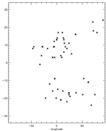
As seen in Fig. 3, the majority of source regions of the CMEs under study lie around the central meridian. This re-sult is in agreement with that of Srivastava and Venkatakrish-nan (2004) and Zhang et al. (2007) who also found that the source regions of CMEs causing major geomagnetic storms lie close to the central meridian (latitude between−22 and 18 degrees and longitude between−30 and 72 degrees). Our study also shows that there is a slight tendency of events to originate from the western part of the solar disc.
Fig. 3. Latitude versus longitude distribution of CMEs sources.
3.3 Dependence of in situ parameters on Dst index with
solar cycle phase
The in situ parameters of our events are analysed within event groups for different phases of the solar cycle, namely ascend-ing, maximum and descending phase.
The SC 23 phases are as follows: the ascending (June 1997–August 1999); maximum (September 1999–July 2002) with two peaks April 2000 and November 2001, descending (August 2002–January 2006). The intervals June 1996–May 1997 and February 2006–December 2008 represent mini-mum phases of solar activity (Maris and Maris, 2010).
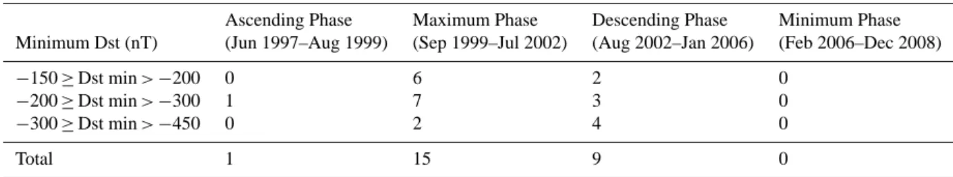
From the analysis of the geomagnetic storms presented in Table 2 and in the Catalog (the electronic material attached to the paper), it was found that in the ascending phase of SC 23 only one major geomagnetic storm (Dst =−205 nT) oc-curred. During the maximum phase, there were 15 major ge-omagnetic storms (60 %), with minimum Dst values ranging between−157 nT and−387 nT. In the descending phase of the solar cycle, there were nine geomagnetic storms with Dst minimum between -181 nT and -422 nT. No major geomag-netic storm was observed at the minimum of solar activity.
Table 2. The distribution of the major geomagnetic storms according to the phase of solar cycle and minimum Dst values.
Ascending Phase Maximum Phase Descending Phase Minimum Phase Minimum Dst (nT) (Jun 1997–Aug 1999) (Sep 1999–Jul 2002) (Aug 2002–Jan 2006) (Feb 2006–Dec 2008)
−150≥Dst min>−200 0 6 2 0
−200≥Dst min>−300 1 7 3 0
−300≥Dst min>−450 0 2 4 0
Total 1 15 9 0
Table 3. Geoeffectiveness of the interplanetary phenomena on the main three phases of the SC 23. Each phase is further sub-divided, de-pending on the strength of the geomagnetic storm: (1)−150 nT≥Dst min>−200 nT; (2)−200 nT≥Dst min>−300 nT; (3)−300 nT≥Dst min>−450 nT.
Ascending Phase Maximum Phase Descending Phase
Type (1) (2) (3) (1) (2) (3) (1) (2) (3) Total
MC – – – 1 – – – – – 1
ICME – – – 1 – – – – – 1
SH+ICME – – – 1 3 1 – 1 – 6
SH+MC – – – 1 2 1 1 1 4 10
CIR – – – – – – – – – 0
Complex – 1 – 2 2 – 1 1 – 7
the maximum phase of the solar cycle, two out of 15 geo-magnetic storms had an minimum Dst<−300 nT, (13 %).
In general, more than one CME is associated with a ma-jor geomagnetic storm, meaning that some CMEs interact in interplanetary space and produce a complex event. But in the case of three severe storms (Dst<−300 nT) (one in July 2000 and two in October 2003), each storm corresponds to one CME. As most of the severe storms (Dst<−300 nT) were observed during the descending phase of SC 23 (four compared with two at maximum of activity), we also exam-ined if the magnitude of the storm is correlated with the mag-netic polarity reversal period. According to Bilenko (2002), the north polar reversal took place in February 2001, or in May 2001 as reported by Durrant and Wilson (2003). For the Southern Hemisphere, the polar reversal took place in September 2001 (Durrant and Wilson, 2003), or in January 2002 as reported by Bilenko (2002). Thus, the poles reversed completely during the maximum of solar activity, before the descending phase started (August 2002) and when the severe storms occurred.
We statistically evaluated various types of disturbances re-sponsible for triggering major geomagnetic storms, depend-ing on the phases of the SC 23 activity. The relationship be-tween the interplanetary phenomena (disturbances) and the geoeffectiveness of the storms are presented in Table 3. The analysis of the geomagnetic storms was done by dividing the Dst index value into three groups: (1) −150 nT≥Dst min>−200 nT; (2) −200 nT≥Dst min>−300 nT; and (3)−300 nT≥Dst min>−450 nT.
Considering the ejecta signatures types in the interplane-tary space, these manifestations can be divided into several classes: MC, ICME, SH+ICME, SH+MC, CIR, and Com-plex (Zhang et al., 2007), as described in Table 1. According to these signatures, we observed that in the ascending phase of SC 23 only one major geomagnetic storm occurred associ-ated with Complex structures. In the maximum phase, 15 ma-jor geomagnetic storms occurred that were produced by MC, ICME, SH+ICME, SH+MC and Complex structures. Finally, in the descending phase, the interplanetary phenomena that caused the nine major geomagnetic storms were SH+ICME, SH+MC and Complex structures.
Most of the storms (ten, 40 %) were produced by SH+MC, seven storms (28 %) by Complex events, six (24 %) by SH+ICME, one storm (4 %) by an MC and one storm (4 %) by an ICME alone.
In conclusion, the statistical study presented above showed that the most geoeffective phenomena are SH+MC, followed by Complex structures and then SH+ICME.
3.4 Correlation between the IP parameters and the
geomagnetic indices
between parameters. The threshold for a correlation to be sig-nificant is 0.05.
We analysed 22 of our 25 ICMEs; three were not included for analysis due to a lack of in situ data (one on 6 Novem-ber 2001 and two on 30 OctoNovem-ber 2003). We computed the correlation coefficients and significance for the most impor-tant parameters of these interplanetary structures (the aver-age values of the interplanetary magnetic field (B), plasma speed (V), proton density and plasma temperature) and the corresponding value of minimum Dst, as shown in Table 4.
We also calculated the correlation coefficients and signif-icance between minimum Dst and the Bz component of the IMF, the plasma speed, Bs·V (where Bs =|Bz|when Bz<0 and Bs = 0 when Bz≥0), the proton density and the plasma temperature, parameters taken at time (t0), one hour earlier (t−1), two hours earlier (t−2) and three hours earlier (t−3) than the time of minimum Dst. Another parameter corre-lated with minimum Dst was the total energy injected into the magnetosphere during the principal phase of the geomag-netic storm (Wε), computed through the Akasofu coupling
function,ε(see Akasofu, 1983). The Akasofu coupling func-tion takes into considerafunc-tion the processes of reconnecfunc-tion within the magnetosphere, as it is considered to be the prin-cipal source of the injected energy (De Lucas et al., 2007):
ε=107V B2l02sin4(θ/2),[J s−1] (2) whereV is the plasma speed,B is the interplanetary mag-netic field (IMF),θis the IMF clock angle in the plane per-pendicular to the Sun–Earth line,l0is the magnetopause ra-dius (l0=7RE),θ=tan−1(By/Bz).
Wε= tm Z
tb
εdt ,[J] (3)
where Wε is obtained by integrating ε over the principal
phase of each geomagnetic storm, from the beginning of the storm (tb) to the time when the minimum Dst was registered (tm). All units are in international system (SI) units of mea-surement.
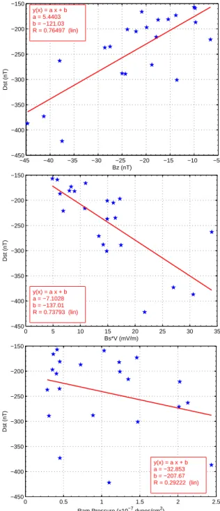
The best correlation coefficients and significance with minimum Dst were found for Bz registered two and three hours earlier than minimum Dst (correlation coefficient (r) of 0.76 and, 0.68 respectively; significance of 3.3×10⁻⁵and 5.1×10⁻⁴) respectively, for Bs·V (r= −0.74; significance = 8.8×10⁻⁵) and for the average value of B (r= −0.66; significance of 9×10⁻⁴). Also, for the total energy injected into the magnetosphere parameter,Wεhad a good correlation
with minimum Dst (r= −0.71, significance = 2.1×10⁻⁴). No significant correlation was found for the plasma tempera-ture and proton density with the strength of the geomagnetic storm.
In Fig. 4 we graphically represent Dst versus Bz (top panel) and Dst versus Bs·V (middle panel). The IP param-eters (Bz andV) are measured two hours before minimum
−45 −40 −35 −30 −25 −20 −15 −10 −5
−450 −400 −350 −300 −250 −200 −150
Bz (nT)
Dst (nT)
y(x) = a x + b a = 5.4403 b = −121.03 R = 0.76497 (lin)
0 5 10 15 20 25 30 35
−450 −400 −350 −300 −250 −200 −150
Bs*V (mV/m)
Dst (nT)
y(x) = a x + b a = −7.1028 b = −137.01 R = 0.73793 (lin)
0 0.5 1 1.5 2 2.5
−450 −400 −350 −300 −250 −200 −150
Ram Pressure (x10−7 dynes/cm2)
Dst (nT)
y(x) = a x + b a = −32.853 b = −207.67 R = 0.29222 (lin)
Fig. 4. Graphic representation of Dst versus various ICME param-eters: Bz vs. Dst (top panel, recorded two hours before minimum Dst), Bs·V vs. Dst (middle panel, recorded two hours before min-imum Dst) and ram pressure vs. Dst (bottom panel, recorded three hours before minimum Dst). The values of Bs·V are multiplied by 10−3.
Table 4. The correlation and significance between the interplanetary structures parameters and the minimum value of Dst. The interplanetary parameters are calculated at the same time as the Dst minimum (t0), one hour (t−1), two (t−2) and three hours earlier, respectively.
Correlation coefficient (r) [Significance]
No Crt. IP parameters IP average IP att0 IP att−1 IP att−2 IP att−3
1. B −0.66 [9.3×10⁻⁴] – – – –
2. Bz – 0.09 [6.7×10⁻¹] 0.46 [2.9×10⁻²] 0.76 [3.3×10⁻⁵] 0.68 [5.1×10⁻⁴] 3. V −0.37 [9.1×10⁻²] −0.20 [3.6×10⁻¹] −0.21 [3.5×10⁻¹] −0.21 [3.3×10⁻¹] −0.29 [1.9×10⁻¹] 4. Bs·V – −0.28 [2.0×10⁻¹] −0.49 [2.1×10⁻²] −0.74 [8.8×10⁻⁵] −0.74 [7.3×10⁻⁵] 5. Ram pressure – −0.15 [4.9×10⁻¹] −0.26 [2.3×10⁻¹] −0.07 [7.3×10⁻¹] −0.29 [1.8×10⁻¹] 6. Proton density −0.25 [2.6×10⁻¹] −0.07 [7.5×10⁻¹] −0.13 [5.7×10⁻¹] 0.07 [7.4×10⁻¹] −0.09 [6.9×10⁻¹] 7. Plasma temperature −0.23 [3.1×10⁻¹] 0.16 [4.8×10⁻¹] 0.18 [4.1×10⁻¹] 0.03 [8.9×10⁻¹] 0.01 [9.6×10⁻¹]
8. Wε −0.71 [2.1×10⁻⁴] – – – –
−20 −10 0 10 20 30 40
−250 −200 −150 −100 −50 0
Dst(nT)
0 −25
−20 −15 −10 −5 0 5
Time (hours)
Bz (nT)
−20 −10 0 10 20 30 40
−250 −200 −150 −100 −50 0
Dst(nT)
0 20
30 40 50 60 70 80
Time (hours)
Kp(x10)
−20 −10 0 10 20 30 40
−250 −200 −150 −100 −50 0
Dst(nT)
0 0
2 4 6 8 10 12 14
x 1012
Time (hours)
Akasofu (J/s)
−20 −10 0 10 20 30 40
20 30 40 50 60 70 80
Kp(x10)
0 0
2 4 6 8 10 12 x 1012
Time (hours)
Akasofu (J/s)
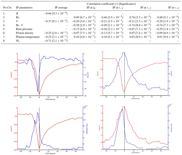
Fig. 5. Superposed epoch analysis for the hourly mean values of Dst and Bz (upper left panel), Dst and Akasofu coupling function (lower left panel) and for the 3-hourly mean values of Dst and Kp (upper right panel), Kp and Akasofu coupling function (lower right panel).
indicates a weak dependence for this pair of parameters. This is different from the result of Srivastava and Venkatakrishnan (2004) who found a better correlation between the two quan-tities.
The minimum Dst versus proton density and the minimum Dst versus plasma temperature, values taken in the same manner as in the upper panels cases, do not show any cor-relation.
Even if the amount of data considered for this study was small (25), it is obvious that certain ICME parameters have a good correlation with the Dst index and thus the intensity of the geomagnetic storm.
3.5 Superposed epoch analysis
48 h after the minimum, as this interval is sufficient to reveal the changes and the evolution of the studied parameters.
To have a better overview, we represented two parame-ters on each plot in Fig. 5. For this purpose, we computed the hourly mean values of Dst index (red line) and Bz (blue line), in the upper left panel and the Dst index (red line) and Akasofu coupling function (blue line), in the lower left panel. Due to the fact that the Kp index is determined on a three-hourly interval, we calculated the 3-hourly mean values of Dst and Akasofu coupling function in order to superpose these parameters onto the Kp index values. We represented the Dst index (red line) and Kp index (blue line) in the upper right panel, and the Kp index (red line) and Akasofu coupling function (blue line) in the lower right panel of Fig. 5. All the values are averages of the 22 events.
The superposed epoch analysis revealed the strong depen-dence of the geomagnetic storm intensity on the southward component of the interplanetary magnetic field, Bz, which leads to magnetic reconnection between the IP structures and Earth’s front-side magnetic field. This strong dependence be-tween the storm intensity and Bz has been well established by the past studies (see, e.g. Wu and Lepping, 2002; Srivas-tava and Venkatakrishnan, 2004; Echer et al., 2008).
A tight dependence between the Akasofu coupling func-tion and both the Dst and Kp values is also evident (see, e.g. Akasofu, 1983; De Lucas et al., 2007). This fact reveals the significant role played by the reconnection in the amount of the energy injected into the magnetosphere in the main phase of each geomagnetic storm.
Upper-right panel of Fig. 5 shows that Kp value increases more rapidly than the decrease of the Dst index, revealing the fact that the field at higher latitudes is disturbed before the field around the Earth’s equator (see e.g. Davis et al., 1997).
4 Summary
The aim of this study was to survey the major geomagnetic storms that took place in SC 23. We analysed the sources, the kinematics and the interplanetary parameters of 57 CMEs that likely caused 25 major geomagnetic storms in solar cycle 23.
All the 57 CMEs were halos and were directed towards Earth. The majority of them emerged complex active regions (βγ orβγ δmagnetic configurations).
The associated flares had a wide energy range, from C2.0 to X17.2. No correlation was found between the geoeffec-tiveness and the importance of a flare.
The CME speed analysis revealed that the projected speeds gave a better estimate of the observed travel time than the ones calculated from a self-similarly expending sphere model. The possible explanations are that the model used to derive the true speed is too simple and/or the CME propa-gates with the same speed in all directions. The CMEs in this study show both acceleration and deceleration while
propagating in interplanetary space due to the interaction with the ambient solar wind or/and the interaction with other CMEs.
The distribution of the major geomagnetic storms over different phases of SC 23 showed that there were no ma-jor storms during the cycle minimum, only one storm with clear solar signatures in the ascending phase, fifteen during the maximum, and nine in the descending phase.
Overall, ten storms (40 %) were produced by SH+MC, seven storms (28 %) by Complex structures, six (24 %) by SH+ICME, one storm (4 %) by an MC and one storm (4 %) by an ICME.
The best correlation coefficients and significance were found between minimum value of Dst and Bz measured two and three hours earlier than minimum Dst. A good correla-tion was also found between the total energy injected into the magnetosphere and Dst. No significant correlation was found between the solar wind plasma temperature, proton density and the strength of the geomagnetic storm.
The superposed epoch analysis revealed the strong depen-dence of the geomagnetic storm intensity to the southward component of the interplanetary magnetic field, Bz, and to the Akasofu coupling function, demonstrating the significant role played by the reconnection between interplanetary and geomagnetic fields and thus the amount of the energy in-jected into the magnetosphere in the main phase of each geo-magnetic storm (see also, Gonzalez and Echer, 2005; Zhang et al., 2007; Echer et al., 2008). The analysis also showed that the field at higher latitudes is disturbed earlier than the field around the Earth equator.
Supplementary material related to this article is
available online at: http://www.ann-geophys.net/31/1285/ 2013/angeo-31-1285-2013-supplement.pdf.
Acknowledgements. This research was supported from the CNC-SIS project TE 2, No. 73/11.08.2010. We acknowledge the use of SOHO, ACE and geomagnetic data. We thank the anonymous ref-erees for their useful comments, which greatly improved the paper. Topical Editor M. Pinnock thanks N. Srivastava and one anony-mous referee for their help in evaluating this paper.
References
Akasofu, S.-I.: Solar-wind disturbances and the solar-wind magne-tosphere energy coupling function, Space Sci. Rev., 34, 173–183, 1983.
Bilenko, I. A.: Coronal holes and the solar polar field reversal, As-tron. Astrophys., 396, 657–666, 2002.
Burlaga, L. F., Klein, L., Sheeley Jr., N. R., Michels, D. J., Howard, R. A., Koomen, M. J., Schwenn, R., and Rosenbauer, H.: A mag-netic cloud and a coronal mass ejection, Geophys. Res. Lett., 9, 1317–1320, 1982.
Cremades, H. and Bothmer, V.: Geometrical Properties of Coro-nal Mass Ejections, IAU Symposium Proceedings of the Inter-national Astronomical Union 226, Held 13–17 September, Bei-jing, edited by: Dere, K., Wang, J., and Yanm, Y., Cambridge: Cambridge University Press, 48–54, 2005.
Davis, C. J., Wild, M. N., Lockwood, M., and Tulunay, Y. K.: Ionospheric and geomagnetic responses to changes in IMF BZ: a superposed epoch study, Ann. Geophys., 15, 217–230, doi:10.1007/s00585-997-0217-9, 1997.
De Lucas, A., Gozales, W. D., Echer, E., Guarnieri, F. L., Dal Lago, A., da Silva, M. R., Vieira, L. E. A., and Schuch, N. J.: Energy balance during intense and super-intense magnetic storms using an Akasofuε parameter corrected by the solar wind dynamic pressure, J. Atmos. Sol.-Terr. Phy., 69, 1851–1863, 2007. Durrant, C. J. and Wilson, P. R.: Observations and Simulations of
the Polar Field Reversals in Cycle 23, Solar Phys., 214, 23–39, 2003.
Echer, E., Gonzalez, W. D., Tsurutani, B. T., and Gonzalez, A. L. C.:Interplanetary conditions causing intense geomagnetic storms (Dst≤100 nT) during solar cycle 23 (1996–2006), J. Geophys. Res., 113, A05221, doi:10.1029/2007JA012744, 2008.
Forsyth, R. J., Rees, A., Balogh, A., and Smith, E. J.: Magnetic Field Observations of Transient Events at Ulysses, 1996–2000, Space Sci. Rev., 97, 217–220, 2001.
Gonzalez, W. D. and Echer, E.: A study on the peak Dst and peak negative Bz relationship during intense geomagnetic storms, Geophys. Res. Lett., 32, L18103, doi:10.1029/2005GL023486, 2005.
Gonzalez, W. D., Joselyn, J. A., Kamide, Y., Kroehl, H. W., Ros-toker, G., Tsurutani, B. T., and Vasyliunas, V. M.: What is a geo-magnetic storm?, J. Geophys. Res., 99, 5771–5792, 1994. Gopalswamy, N.: Solar connections of geoeffective magnetic
struc-tures, J. Atmos. Sol.-Terr. Phy., 70, 2078–2100, 2008.
Gopalswamy, N., Yashiro, S., Kaiser, M. L., Howard, R. A., and Bougeret, J.-L.: Radio Signatures of Coronal Mass Ejection In-teraction: Coronal Mass Ejection Cannibalism?, Astrophys. J., 548, L91–L94, 2001.
Gopalswamy, N., Yashiro, S., Michalek, G., Xie, H., Lepping, R. P., and Howard, R. A.: Solar source of the largest geo-magnetic storm of cycle 23, Geophys. Res. Lett., 32, L12S09, doi:10.1029/2004GL021639, 2005.
Gopalswamy, N., Yashiro, S., and Akiyama, S.: Geoeffectiveness of halo coronal mass ejections, J. Geophys. Res., 112, A06112, doi:10.1029/2006JA012149, 2007.
Gopalswamy, N., Akiyama, S., Yashiro, S., Michalek, G., and Lep-ping, R. P.: Solar sources and geospace consequences of inter-planetary magnetic clouds observed during solar cycle 23, J. At-mos. Sol.-Terr. Phy., 70, 245–253, 2008.
Gosling, J. T., Asbridge, J. R., Bame, S. J., Feldman, W. C., and Zwickl, R. D.: Observations of large fluxes of He/+/ in the solar wind following an interplanetary shock, J. Geophys. Res., 85, 3431–3434, 1980.
Guo, J., Feng, X., Emery, B. A., Zhang, J., Xiang, C., Shen, F., and Song, W.: Energy transfer during intense geomag-netic storms driven by interplanetary coronal mass ejections
and their sheath regions, J. Geophys. Res., 116, A05106, doi:10.1029/2011JA016490, 2011.
Harrison, R. A.: The nature of solar flares associated with coronal mass ejections, A&A, 304, 585–591, 1995.
Hudson, H. S., Bougeret, J.-L., and Burkepile, J.: Coronal Mass Ejections: Overview of Observations, Space Sciences Series of ISSI, 21, ISBN 978-0-387-45086-5, Springer, 13–30, 2006. Huttunen, K. E. J., Koskinen, H. E. J., Schwenn, R., and dal Lago,
A.: Causes of major magnetic storms near the latest solar maxi-mum, in: ESA SP-506, 1, Noordwijk, edited by: Wilson, A., ESA Publications Division, ISBN 92-9092- 816-6, 2002.
Jian, L., Russell, C. T., Luhmann, J. G., and Skoug, R. M.: Proper-ties of Interplanetary Coronal Mass Ejections at One AU During 1995–2004, Solar Phys., 239, 393–436, 2006.
Maris, G. and Maris, O.: Rapid solar wind and geomagnetic vari-ability during the ascendant phases of the 11-yr solar cycles, So-lar and StelSo-lar Variability: Impact on Earth and Planets, Proceed-ings of the International Astronomical Union, IAU Symposium, 264, 359–362, 2010.
Maris, G., Popescu, M. D., and Mierla, M.: The North-South Asym-metry of Soft X-Ray Solar Flares, Romanian Astronomical Jour-nal, 12, 131–146, 2002.
Michalek, G.: An Asymmetric Cone Model for Halo Coronal Mass Ejections, Solar Phys., 237, 101–118, 2006.
Mierla, M., Besliu-Ionescu, D., Chiricuta, O., Oprea, C., and Maris, G.: Studies of coronal mass ejections that have produced major geomagnetic storms, Sun and Geosphere, 7, 13–16, 2012. Ontiveros, V. and Vourlidas, A.: Quantitative Measurements of
Coronal Mass Ejection-Driven Shocks from LASCO Observa-tions, Astrophys. J., 693, 267–275, 2009.
Rodriguez, L., Woch, J., Krupp, N., Fr¨anz, M., von Steiger, R., Cid, C., Forsyth, R., and Glaßmeier, K.-H.: Freezing-In Temperatures of Oxygen, Carbon and Iron in Magnetic Clouds, Proceedings of the Solar Wind 11/SOHO 16, “Connecting Sun and Heliosphere” Conference (ESA SP-592), 12–17 June 2005 Whistler, Canada, edited by: Fleck, B., Zurbuchen, T. H., and Lacoste, H., p. 759, 2005.
Rouillard, A. P.: Relating white light and in situ observations of coronal mass ejections: A review, J. Atmos. Sol.-Terr. Phy., 73, 1201–1213, 2011.
Schwenn, R., Rosenbauer, H., and Muehlhaeuser, K.-H.: Singly-ionized helium in the driver gas of an interplanetary shock wave, Geophys. Res. Lett., 7, 201–204, 1980.
Srivastava, N. and Venkatakrishnan, P.: Relationship between CME Speed and Geomagnetic Storm Intensity, Geophys. Res. Lett., 29, 1287, doi:10.10292001GL013597, 2002.
Srivastava, N. and Venkatakrishnan, P.: Solar and interplanetary sources of major geomagnetic storms during 1996–2002, J. Geo-phys. Res., 109, A10103, doi:10.1029/2003JA010175, 2004. Srivastava, N., Inhester, B., Mierla, M., and Podlipnik, B.: 3D
Re-construction of the Leading Edge of the 20 May 2007 Partial Halo CME, Solar Phys., 259, 213–225, 2009.
Thernisien, A. F. R., Howard, R. A., and Vourlidas, A.: Modeling of Flux Rope Coronal Mass Ejections, Astrophys. J., 652, 763–773, 2006.
Webb, D. F. and Howard, T. A.: Coronal Mass Ejections: Obser-vations, Living Rev. Solar Phys., 9, 3, doi:10.12942/lrsp-2012-3, 2012.
Wu, C.-C. and Lepping, R. P.: Effects of magnetic clouds on the occurrence of geomagnetic storms: The first 4 years of Wind, J. Geophys. Res., 107, 1314, doi:10.1029/2001JA000161, 2002. Xie, H., Ofman, L., and Lawrence, G.: Cone model for halo CMEs:
Application to space weather forecasting, J. Geophys. Res., 109, A03109, doi:10.1029/2003JA010226, 2004.
Zhang, J., Richardson, I. G., Webb, D. F., Gopalswamy, N., Hut-tunen, E., Kasper, J. C., Nitta, N. V., Poomvises, W., Thomp-son, B. J., Wu, C.-C., Yashiro, S., and Zhukov, A. N.: So-lar and interplanetary sources of major geomagnetic storms (Dst≤ −100 nT) during 1996–2005, J. Geophys. Res., 112, A10102, doi:10.1029/2007JA012321, 2007.
Zhao, X. P., Plunkett, S. P., and Liu, W.: Determination of geo-metrical and kinematical properties of halo coronal mass ejec-tions using the cone model, J. Geophys. Res., 107, 1223, doi:10.1029/2001JA009143, 2002.