The Outdoor Dust Information Node (ODIN) – development and performance assessment of a low cost ambient dust sensor

(1)

AMTD

8, 7511–7533, 2015

ODIN development and performance

G. Olivares and S. Edwards

Title Page

Abstract Introduction

Conclusions References

Tables Figures

◭ ◮

Back Close

Full Screen / Esc

Printer-friendly Version Interactive Discussion

Discussion

P

a

per

|

Discussion

P

a

per

|

Discussion

P

a

per

|

Discussion

P

a

per

|

Atmos. Meas. Tech. Discuss., 8, 7511–7533, 2015 www.atmos-meas-tech-discuss.net/8/7511/2015/ doi:10.5194/amtd-8-7511-2015

This discussion paper is/has been under review for the journal Atmospheric Measurement Techniques (AMT). Please refer to the corresponding final paper in AMT if available.

The Outdoor Dust Information Node

(ODIN) – development and performance

assessment of a low cost ambient dust

sensor

G. Olivares and S. Edwards

National Institute of Water and Atmospheric Research (NIWA), 41 Market Place, Auckland Central 1010, Auckland, New Zealand

Received: 15 June 2015 – Accepted: 30 June 2015 – Published: 22 July 2015

Correspondence to: G. Olivares ([email protected])

(2)

AMTD

8, 7511–7533, 2015

Title Page

Tables Figures

◭ ◮

Back Close

Full Screen / Esc

Discussion

P

a

per

|

Discussion

P

a

per

|

Discussion

P

a

per

|

Discussion

P

a

per

|

Abstract

The large gradients in air quality expected in urban areas present a significant chal-lenge to standard measurement technologies. Small, low-cost devices have been de-veloping rapidly in recent years and have the potential to improve the spatial coverage of traditional air quality measurements. Here we present the first version of the Outdoor

5

Dust Information Node (ODIN) as well as the results of the first real-world measure-ments. The lab tests indicate that the Sharp dust sensor used in the ODIN presents a stable baseline response only slightly affected by ambient temperature. The field tests indicate that ODIN data can be used to estimate hourly and daily PM2.5concentrations

after appropriate temperature and baseline corrections are applied. The ODIN seems

10

suitable for campaign deployments complementing more traditional measurements.

1 Introduction

Global estimates indicate that between 70–90 % of the population is exposed to av-erage annual PM2.5 concentrations that exceed the World Health Organization Air

Quality Guideline of 10 µg m−3(annual average). This translates into between 2.2 and

15

7 million premature deaths year−1

worldwide (Brauer et al., 2012; Lim et al., 2012). A significant source of uncertainty in these estimates is the spatial representative-ness of the measurements used to generate them. The cost of installing and operating air quality monitoring stations means that a small number of measurements are used to represent extensive geographical areas (Wilson et al., 2005; Asian Development Bank,

20

2014). This is particularly relevant in urban areas where large gradients are expected in the concentration of pollutants especially in areas with large density of sources. These gradients can not be resolved if the spatial coverage of the measurements is inadequate (Chow et al., 2002; Holstius et al., 2014; Wilson et al., 2005).

Also, capturing accurate data to assess personal exposure to air pollution is critical

25

(3)

AMTD

8, 7511–7533, 2015

Title Page

Tables Figures

◭ ◮

Back Close

Full Screen / Esc

Discussion

P

a

per

|

Discussion

P

a

per

|

Discussion

P

a

per

|

Discussion

P

a

per

|

Determining exposure in both time and space is challenging as individual behaviour affects daily and long term exposure to air pollution (Wilson et al., 2005). Therefore, health effect studies require accurate, spatially and temporally resolved air quality data. Epidemiological studies often use ambient concentrations at a city level as a proxy for exposure. The spatial and temporal resolution of reported data sets means they

5

are unlikely to adequately reflect individual pollution exposure (Chow et al., 2002). Modelling can partially compensate for the lack of spatial resolution, but in regions with complex topography and meteorology or unevenly distributed and poorly characterised emission sources, model accuracy is constrained (Wilson et al., 2005).

The spatial and temporal resolution of air pollution data sets could be improved by

10

deploying additional sensors to supplement existing monitoring networks. Where previ-ously the cost of doing so was prohibitive, rapid advances in technology in recent years have seen increasing numbers of low cost air pollution sensors available. Individuals and non-regulatory groups have seized the opportunity and developed citizen science initiatives to monitor their local air quality (Egg, 2014; Hart and Martinez, 2006; Smith

15

and Clark, 2013; SPECK, 2015).

Whilst low-cost sensors have increased the accessibility of air pollution data to the general public, the sensors are not without limitations. Instruments used for regula-tory monitoring must meet high standards of precision, accuracy, comparability and traceability (Wang and Brauer, 2014) whereas low cost sensors are often provided

20

without calibration information and have either not been characterised under ambient conditions or tested only for a limited time leaving questions on their long term reli-ability (Snyder et al., 2013). This is not necessarily a problem if the purpose of the measurements is commensurate with the capabilities of the sensors. For example, in some cases qualitative information indicating an increase or decrease of pollutant

lev-25

(4)

AMTD

8, 7511–7533, 2015

Title Page

Tables Figures

◭ ◮

Back Close

Full Screen / Esc

Discussion

P

a

per

|

Discussion

P

a

per

|

Discussion

P

a

per

|

Discussion

P

a

per

|

composition. To date very few low-cost pollution sensors have been evaluated against compliance monitoring instruments (Holstius et al., 2014; Williams et al., 2014).

We have made some progress in the use of low cost sensors for the assessment of personal pollution exposure with the development of the Particles, Activity and Context Monitoring Autonomous Node (PACMAN) for indoor exposure studies (Olivares et al.,

5

2013). In this work we describe the development of the outdoor counterpart of PAC-MAN the Outdoor Dust Information Node (ODIN), a new, low-cost, battery powered sensor package to monitor outdoor particulate concentrations. We also explore the performance of the dust sensor at the heart of ODIN and PACMAN in terms of baseline stability. Finally, we present results of the first field tests of the ODIN co-located with

tra-10

ditional standard instrumentation at a regulatory monitoring site in Christchurch, New Zealand. These tests indicate that the ODIN is able to capture PM2.5 concentrations

once suitable corrections are applied which make it a viable instrument to measure PM in combustion dominated areas complementing traditional measurements.

2 Methods 15

2.1 ODIN

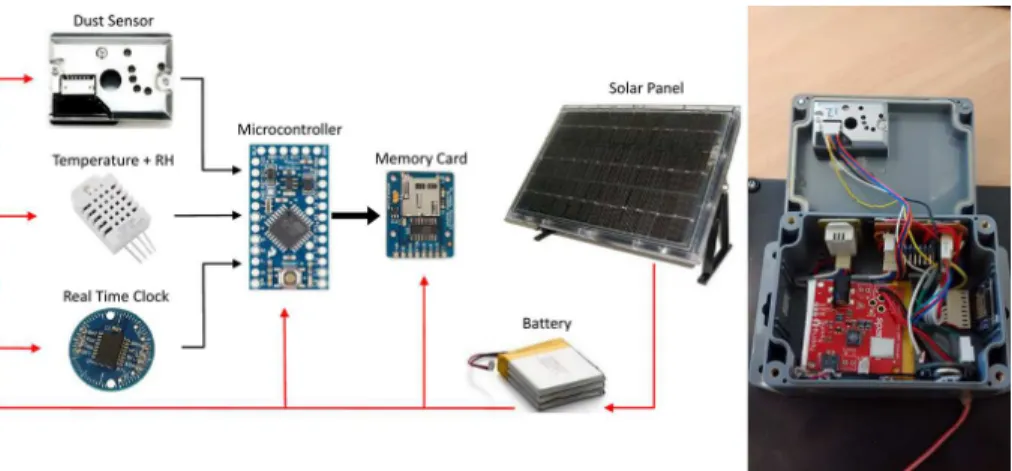
The Outdoor Dust Information Node (ODIN) was developed leveraging on the extensive open source hardware and software communities using readily available components. In very broad terms, the ODIN is a set of sensors that are integrated by a microcon-troller that logs the data. Figure 1 shows a diagram of the operation of ODIN and a view

20

of the internal layout of the device. Power is drawn from either the battery or the so-lar panel depending on the sunshine. To maximize the battery life, the ODIN uses its microcontroller’ssleep mode and only wakes up to take a single measurement every minute.The sensors feed information to the microcontroller which in turn saves it to the memory card. The electric design files are available from Olivares and Edwards (2014)

25

(5)

AMTD

8, 7511–7533, 2015

Title Page

Tables Figures

◭ ◮

Back Close

Full Screen / Esc

Discussion

P

a

per

|

Discussion

P

a

per

|

Discussion

P

a

per

|

Discussion

P

a

per

|

– Dust sensor: the Sharp Optical Dust Sensor GP2Y1010AU0F was selected

be-cause of its low power consumption (SHARP, 2015).The basic measurement prin-ciple of this sensor is infra-red light scattering. An infra-red light emitting diode (IRLED) and a photodetector (PD) are arranged 90◦ to each other around the sensing volume. The particles in the sensing volume scatter the light from the

5

IRLED which is measured by the PD. This sensor requires 5–7 Vdc to operate and outputs a 0–3 Vdc signal proportional to the total dust mass measured. The operation of this sensor is as a 10 ms sampling cycle consisting of a high phase of 0.32 ms and a low phase of 9.68 ms. A single measurement is taken 0.28 ms into the high phase (SHARP, 2015). To smooth the output of this sensor, the

mi-10

crocontroller takes 100 samples of 10 ms each and records their average.

Note that the dust sensor does not have a defined measurement size range but that the upper and lower cut offsizes are controlled by the sensitivity of the internal amplifying circuit. It is expected that this circuit has significant inter-instrument variability as well as its response to depend on the type of aerosol sampled.

15

– Temperature and relative humidity: the AM2302 temperature-humidity sensor

from AOSONG was selected for its size, power consumption and ease of inter-face. According to the manufacturers, the AM2302 is accurate to within 2 % RH and 0.5◦C and it is able to operate in a wide range of conditions (AOSONG, 2015).

– Microcontroller: Sparkfun’s Arduino Pro Mini (Sparkfun, 2014) based on the

AT-20

Mega328 microcontroller was selected primarily because of its ease of use and the programming libraries available for the Arduino system. The firmware used on this microcontroller is available in the project’s GitHub repository (Olivares and Edwards, 2014).

– Memory: a 2 GB micro SD card is used to log the data. Adafruit’s micro SD card

25

(6)

AMTD

8, 7511–7533, 2015

Title Page

Tables Figures

◭ ◮

Back Close

Full Screen / Esc

Discussion

P

a

per

|

Discussion

P

a

per

|

Discussion

P

a

per

|

Discussion

P

a

per

|

– Clock: the DS3231 based temperature compensated RTC Chronodot v2.0

(Macetech, 2013) was used to keep track of time. This component is documented to have a drift smaller than one minute per year. A specific library was used to communicate with this component (Maks, 2012).

– Power: a lithium ion polymer battery pack (3.7 V) delivers the power required for

5

the unit. A 6 Ah battery is capable of powering the system for six weeks. A so-lar panel was added to the design which under ideal conditions of sunshine, is capable of powering the system as well as recharging the battery for long term deployments. Unfortunately the chosen combination of solar panel and charging circuit was unable to recover the battery so in future revisions a new solution will

10

be tested.

Figure 1 also shows the internal layout of the ODIN. As the ODIN is a passive instru-ment, i.e. there is no forced air sample, the dust sensor is located against the wall of the enclosure with its opening directly towards the outside of the instrument, protected by a rain shield and a coarse metal mesh.

15

The cost of the materials for the prototype ODIN is less than USD 300 (June 2015) and each unit takes about three hours to put together.

2.2 Deployments

Several short deployments were used to capture the data presented here. The first one was aimed at characterise the zero response of the dust sensor at the heart of the

20

ODIN. Eight Sharp dust sensors were set up in a custom made, sealed and uninsulated enclosure and placed in a controlled environment for five days at a temperature of 22±1◦C and a relative humidity of 50±5 %. Following this deployment, the same eight

units were placed outdoors in the same sealed container but exposed to sunshine. The sensors were subject to temperatures ranging from 6 to 26◦C. More than 4000 records

25

(7)

AMTD

8, 7511–7533, 2015

Title Page

Tables Figures

◭ ◮

Back Close

Full Screen / Esc

Discussion

P

a

per

|

Discussion

P

a

per

|

Discussion

P

a

per

|

Discussion

P

a

per

|

To evaluate the response of the ODIN to woodsmoke and assess its performance against standard air quality instrumentation, one unit (ODIN_01) was located at En-vironment Canterbury’s1 air quality monitoring site at Coles Place (−43.511236◦S;

172.633687◦W) between the 24 July and the 14 August 2014. The unit was attached to the meteorological mast at the same height as the inlets for the PM10 and PM2.5

5

instruments at the site (Fig. 2). The data were manually downloaded from the internal memory at the end of the test period.

Data from the air quality monitoring station were obtained from Environment Can-terbury. These data were provided before the normal QA process as 60 min moving average, every 10 min of, PM₁₀, PM_2.5measured by a TEOM-FDMS instrument, wind

10

speed and direction and air temperature. The details of these measurements are de-scribed by Aberkane et al. (2010).

2.3 Data analysis

All the data analysis was done using R Team (2014) and the Openair R package (Carslaw and Ropkins, 2012). The raw data are available from Olivares (2015a) and

15

the analysis scripts are available from Olivares (2015b).

The baseline of each instrument was obtained by averaging all the measurements taken during the temperature controlled baseline deployment described above. This baseline was then subtracted from the raw measurements to obtain thebaseline

cor-rectedsignal. The temperature response of the sensors was estimated using data from

20

the variable temperature baseline deployment. A linear regression between the

base-line correctedsignal and the ambient temperature in the enclosure was performed to

describe the effect of ambient temperature on the response of the Sharp dust sensors. For the co-location deployment the data analysis included the following: we first re-moved baseline drift, then corrected for temperature effects and then found the

calibra-25

tion coefficients to approximate PM2.5. 1

(8)

AMTD

8, 7511–7533, 2015

Title Page

Tables Figures

◭ ◮

Back Close

Full Screen / Esc

Discussion

P

a

per

|

Discussion

P

a

per

|

Discussion

P

a

per

|

Discussion

P

a

per

|

More in detail, the baseline drift was estimated from the linear trend of the raw re-sponse from ODIN. This baseline was subtracted from the raw ODIN output.

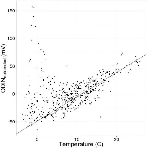
Then, a temperature correction was applied by first finding the linear regression be-tween the de-trended ODIN signal and the instrument temperature. This was done by considering only data above 10◦C. Figure 3 shows that above 10◦C the temperature

5

effect dominates the ODIN response. The data were then corrected by subtracting the linear regression with the temperature from the de-trended ODIN output.

To obtain the correction coefficients to estimate PM2.5, this de-trended and

tempera-ture corrected ODIN signal was used in a linear regression with PM2.5as the dependent

variable and the ODIN signal. To explore the stability of this correction, the linear

re-10

gression was performed on the first 1/3 of the data while the error estimate (RMSE) was calculated using the whole dataset.

3 Results

3.1 Dust sensor behaviour

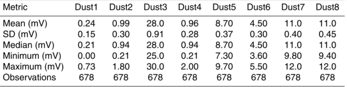
Table 1 shows the results of the baseline test for the eight sensors tested and highlights

15

the inter-instrument variability for the Sharp dust sensor with the range of baselines be-tween 0.24 to 28 mV. For each sensor, the standard deviation of the baseline estimate suggests a relatively stable baseline for the sensors tested.

In our previous work with similar sensors we found a linear relationship between the baseline response of the dust sensor and ambient temperature in field deployments

20

(Olivares et al., 2013). Our original hypothesis was that this interference by temperature was a property of the sensor so, as described above, we placed several units in a clean environment exposed to a range of temperatures.

If the effect of ambient temperature on the Sharp dust sensor readings was related to the sensor itself we would expect that there would be a significant increase in their

25

(9)

AMTD

8, 7511–7533, 2015

Title Page

Tables Figures

◭ ◮

Back Close

Full Screen / Esc

Discussion

P

a

per

|

Discussion

P

a

per

|

Discussion

P

a

per

|

Discussion

P

a

per

|

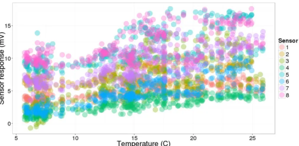
As shown in Fig. 4, ambient temperature appears to change the response of the sensors by around 0.3 mV for every 1◦C. This, however is a much weaker response to temperature than what is found when using the sensor as part of the ODIN. Table 2 shows that the temperature correction applied to the ambient data is of 4.4 mV for every 1◦C. This suggests that the impact of temperature on the response from the

5

Sharp dust sensor is dominated by impacts on the aerosol instead of being a property of the devices. However, future tests will further explore this behaviour.

3.2 ODIN’s performance evaluation

Figure 5 shows that the raw ODIN data show a significant baseline drift and they only capture a small fraction of the features observed in the PM2.5time series. The

base-10

line correction showed a significant drift of almost−30 % during the deployment

(Ta-ble 2). After removing the baseline drift, the temperature correction was estimated as 4.4 mV◦C−1 (Table 2) which, as noted above, is significantly higher than what was ob-tained in clean conditions but similar to what was observed by our group in a previous work (Olivares et al., 2013).

15

Table 2 shows that, after applying the baseline and temperature corrections, a cali-bration factor of 0.6 and an offset of 19 µg m−3is sufficient for the ODIN data to capture most of the variability of PM2.5. Figure 6 shows that the corrected ODIN data captured

both the timing and intensity of all the high concentration events observed in the PM_2.5 data. However, for PM2.5concentrations below 25 µg m−

3

the scatter plot shows a less

20

defined relationship between ODIN and PM_2.5.

Figure 6 also shows that the correction calculated for the beginning of the deploy-ment significantly overestimates the low concentrations observed towards the end of the dataset. This could be due to a residual baseline drift not accounted for by the method used but it does not seem to affect the fit for the higher concentrations.

25

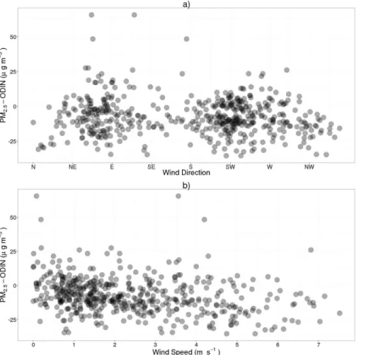
Finally, and to evaluate the behaviour of the ODIN’s inlet, we compared the error in the ODIN estimate (PM2.5−ODIN) with the observed wind speed and direction.

(10)

AMTD

8, 7511–7533, 2015

Title Page

Tables Figures

◭ ◮

Back Close

Full Screen / Esc

Discussion

P

a

per

|

Discussion

P

a

per

|

Discussion

P

a

per

|

Discussion

P

a

per

|

with wind speed. This difference in higher wind speeds could be related to a different source mix than in low wind speeds which typically occur during night time (Aberkane et al., 2010). However, PM2.5concentrations are generally lower in high wind speeds

which, as indicated before, is closer to the detection limit of the Sharp dust sensor.

4 Conclusions 5

The small, low-cost dust monitor ODIN, based on an optical dust sensor has been shown to be able to capture most of the features of the PM_2.5 time series in a wood-smoke impacted area after suitable baseline and temperature corrections are applied. In controlled conditions, the optical dust sensor used in ODIN was shown to have a stable baseline with a small dependence with ambient temperature. However, field

10

data indicates a significant baseline drift and temperature interference. The baseline drift of nearly 30 % in three weeks indicates that regular checks will be required if the ODIN is to be used for extended periods of time.

The fact that the temperature interference observed in the field tests was more sig-nificant than that observed in lab conditions suggests that the changes in the response

15

of the ODIN to ambient temperature are related to the nature of the aerosol sampled and not only to the sensor themselves. This has implications for the transferability of the correction factors to other locations.

Also, the performance of the ODIN is worst for PM_2.5concentrations below 25 µg m−3. This is to be expected as the datasheet of the Sharp dust sensor has a response curve

20

starting at 100 µg m−3. This is a common characteristic of low-cost sensors (Wang and Brauer, 2014) and one should be cautious when using these sensors in low-concentration environments as their response may reflect more their noise than a real measurement.

A simple test of the performance of ODIN against wind speed and direction found that

25

(11)

AMTD

8, 7511–7533, 2015

Title Page

Tables Figures

◭ ◮

Back Close

Full Screen / Esc

Discussion

P

a

per

|

Discussion

P

a

per

|

Discussion

P

a

per

|

Discussion

P

a

per

|

fact that high wind speeds relate to low concentrations, where the Sharp dust sensor perform worst, and that a different source mix may be dominant in those conditions.

Nevertheless, the ODIN is shown to be a useful complement to regulatory mea-surements for campaigns and its calibration parameters are stable for deployments of around one month.

5

The next steps in understanding the response of the ODIN to urban aerosols are to explore more in detail the performance of the Sharp dust sensor to specific aerosol pop-ulations (size and composition), explore the inter-instrument variability and the drivers for the baseline drift and temperature interference found here. We also expect to ex-plore the transferability of correction coefficients with data currently being captured in

10

Auckland and Christchurch and it is expected to generate results by September 2015. Future versions of the ODIN are expected to include distributed telemetry for high density deployments at a city scale as well as improved energy efficiency for long term deployments.

Acknowledgements. The development of ODIN was funded through NIWA’s Atmosphere and

15

Health 2013-14 programme (ATHS1301). The ODIN deployments and data analysis were funded through NIWA’s Impacts of Air Pollutants 2014-15 programme (CAAP1504). Also, we gratefully acknowledge the support from Environment Canterbury through Teresa Aberkane in giving us access to Christchurch’s air quality monitoring sites and data.

References 20

Aberkane, T., Harvey, M., and Webb, M.: Annual Ambient Air Quality Monitoring Report 2009, no. U04/58 in Environment Canterbury Technical Report, Environ-ment Canterbury, Christchurch, available at: http://www.crc.govt.nz/publications/Reports/ annual-ambient-air-quality-monitoring-report-2009-000310.pdf (last access: 8 Juy 2014), 2010. 7517, 7520

25

(12)

AMTD

8, 7511–7533, 2015

Title Page

Tables Figures

◭ ◮

Back Close

Full Screen / Esc

Discussion

P

a

per

|

Discussion

P

a

per

|

Discussion

P

a

per

|

Discussion

P

a

per

|

Air Quality Egg: Air Quality Egg, available at: http://airqualityegg.com/, last access: 4 July 2014. 7513

AOSONG: Aosong(Guangzhou) Electronics Co.,Ltd., available at: http://www.aosong.com/en/ products/details.asp?id=117, last access: 19 May 2015. 7515

Asian Development Bank: Improving Air Quality Monitoring in Asia: a Good Practice

Guid-5

ance, Tech. rep., Asian Development Bank, Mandaluyong City, Philippines, available at: http://cleanairasia.org/portal/sites/default/files/improving_aqmt_in_asia.pdf (last access: 19 May 2015), 2014. 7512

Brauer, M., Amann, M., Burnett, R. T., Cohen, A., Dentener, F., Ezzati, M., Henderson, S. B., Krzyzanowski, M., Martin, R. V., Van Dingenen, R., van Donkelaar, A., and Thurston, G. D.:

10

Exposure assessment for estimation of the global burden of disease attributable to outdoor air pollution, Environ. Sci. Technol., 46, 652–660, doi:10.1021/es2025752, 2012. 7512 Carslaw, D. C. and Ropkins, K.: openair – an R package for air quality data analysis, Environ.

Modell. Softw., 27–28, 52–61, doi:10.1016/j.envsoft.2011.09.008, 2012. 7517

Chow, J. C., Engelbrecht, J. P., Watson, J. G., Wilson, W. E., Frank, N. H., and Zhu, T.: Designing

15

monitoring networks to represent outdoor human exposure, Chemosphere, 49, 961–978, doi:10.1016/S0045-6535(02)00239-4, 2002. 7512, 7513

Hart, J. K. and Martinez, K.: Environmental sensor networks: a revolution in the earth system science?, Earth-Sci. Rev., 78, 177–191, doi:10.1016/j.earscirev.2006.05.001, 2006. 7513 Holstius, D. M., Pillarisetti, A., Smith, K. R., and Seto, E.: Field calibrations of a low-cost aerosol

20

sensor at a regulatory monitoring site in California, Atmos. Meas. Tech., 7, 1121–1131, doi:10.5194/amt-7-1121-2014, 2014. 7512, 7514

Lim, S. S., Vos, T., Flaxman, A. D., Danaei, G., Shibuya, K., Adair-Rohani, H., AlMazroa, M. A., Amann, M., Anderson, H. R., Andrews, K. G., Aryee, M., Atkinson, C., Bacchus, L. J., Ba-halim, A. N., Balakrishnan, K., Balmes, J., Barker-Collo, S., Baxter, A., Bell, M. L., Blore, J. D.,

25

Blyth, F., Bonner, C., Borges, G., Bourne, R., Boussinesq, M., Brauer, M., Brooks, P., Bruce, N. G., Brunekreef, B., Bryan-Hancock, C., Bucello, C., Buchbinder, R., Bull, F., Bur-nett, R. T., Byers, T. E., Calabria, B., Carapetis, J., Carnahan, E., Chafe, Z., Charlson, F., Chen, H., Chen, J. S., Cheng, A. T.-A., Child, J. C., Cohen, A., Colson, K. E., Cowie, B. C., Darby, S., Darling, S., Davis, A., Degenhardt, L., Dentener, F., Des Jarlais, D. C., Devries, K.,

30

(13)

Gio-AMTD

8, 7511–7533, 2015

Title Page

Tables Figures

◭ ◮

Back Close

Full Screen / Esc

Discussion

P

a

per

|

Discussion

P

a

per

|

Discussion

P

a

per

|

Discussion

P

a

per

|

vannucci, E., Gmel, G., Graham, K., Grainger, R., Grant, B., Gunnell, D., Gutierrez, H. R., Hall, W., Hoek, H. W., Hogan, A., Hosgood, H. D., Hoy, D., Hu, H., Hubbell, B. J., Hutch-ings, S. J., Ibeanusi, S. E., Jacklyn, G. L., Jasrasaria, R., Jonas, J. B., Kan, H., Kanis, J. A., Kassebaum, N., Kawakami, N., Khang, Y.-H., Khatibzadeh, S., Khoo, J.-P., Kok, C., Laden, F., Lalloo, R., Lan, Q., Lathlean, T., Leasher, J. L., Leigh, J., Li, Y., Lin, J. K., Lipshultz, S. E.,

5

London, S., Lozano, R., Lu, Y., Mak, J., Malekzadeh, R., Mallinger, L., Marcenes, W., March, L., Marks, R., Martin, R., McGale, P., McGrath, J., Mehta, S., Memish, Z. A., Men-sah, G. A., Merriman, T. R., Micha, R., Michaud, C., Mishra, V., Hanafiah, K. M., Mok-dad, A. A., Morawska, L., Mozaffarian, D., Murphy, T., Naghavi, M., Neal, B., Nelson, P. K., Nolla, J. M., Norman, R., Olives, C., Omer, S. B., Orchard, J., Osborne, R., Ostro, B.,

10

Page, A., Pandey, K. D., Parry, C. D., Passmore, E., Patra, J., Pearce, N., Pelizzari, P. M., Petzold, M., Phillips, M. R., Pope, D., Pope, C. A., Powles, J., Rao, M., Razavi, H., Re-hfuess, E. A., Rehm, J. T., Ritz, B., Rivara, F. P., Roberts, T., Robinson, C., Rodriguez-Portales, J. A., Romieu, I., Room, R., Rosenfeld, L. C., Roy, A., Rushton, L., Salomon, J. A., Sampson, U., Sanchez-Riera, L., Sanman, E., Sapkota, A., Seedat, S., Shi, P., Shield, K.,

15

Shivakoti, R., Singh, G. M., Sleet, D. A., Smith, E., Smith, K. R., Stapelberg, N. J., Steen-land, K., Stöckl, H., Stovner, L. J., Straif, K., Straney, L., Thurston, G. D., Tran, J. H., Van Dingenen, R., van Donkelaar, A., Veerman, J. L., Vijayakumar, L., Weintraub, R., Weiss-man, M. M., White, R. A., Whiteford, H., Wiersma, S. T., Wilkinson, J. D., Williams, H. C., Williams, W., Wilson, N., Woolf, A. D., Yip, P., Zielinski, J. M., Lopez, A. D., Murray, C. J.,

20

and Ezzati, M.: A comparative risk assessment of burden of disease and injury attributable to 67 risk factors and risk factor clusters in 21 regions, 1990–2010: a systematic analysis for the Global Burden of Disease Study 2010, Lancet, 380, 2224–2260, doi:10.1016/S0140-6736(12)61766-8, 2012. 7512

Macetech: chronodot_v2.0, macetech documentation, available at: http://docs.macetech.com/

25

doku.php/chronodot%5C_v2.0 (last access: 19 May 2015), 2013. 7516

Maks, S.: Stephanie-Maks/Arduino-Chronodot, available at: https://github.com/Stephanie-Maks/Arduino-Chronodot (last access: 1 May 2015), 2012. 7516

McKone, T. E., Ryan, P. B., and Özkaynak, H.: Exposure information in environmental health research: current opportunities and future directions for particulate matter, ozone, and toxic

30

air pollutants, J. Expo. Sci. Env. Epid., 19, 30–44, doi:10.1038/jes.2008.3, 2008. 7512 Olivares, G.: ODIN Test and Co-Location Data, available at: http://figshare.com/articles/ODIN_

(14)

AMTD

8, 7511–7533, 2015

Title Page

Tables Figures

◭ ◮

Back Close

Full Screen / Esc

Discussion

P

a

per

|

Discussion

P

a

per

|

Discussion

P

a

per

|

Discussion

P

a

per

|

Olivares, G.: ODIN Analysis Script June 2015, available at: http://figshare.com/articles/ODIN_ analysis_script_June_2015/1449236 (last access: 15 June 2015), 2015b. 7517

Olivares, G. and Edwards, S.: ODIN Firmware, doi:10.6084/m9.figshare.1094459, 2014. 7514, 7515, 7527

Olivares, G., Longley, I., and Coulson, G.: Development of a Low-Cost Device for

Ob-5

serving Indoor Particle Levels Associated With Source Activities in the Home, available at: http://figshare.com/articles/Development_of_a_low_cost_device_for_observing_indoor_ particle_levels_associated_with_source_activities_in_the_home/646186 (last access: 27 August 2014), 2013. 7514, 7518, 7519

SHARP: GP2Y1010AU0F – Air Sensor, Sharp Microelectronics Europe, available at: http:

10

//www.sharpsme.com/optoelectronics/sensors/air-sensors/GP2Y1010AU0F, last access: 19 May 2015. 7515

Smith, P. and Clark, M.: Microsampling Air Pollution, available at: http://well.blogs.nytimes.com/ 2013/06/03/microsampling-air-pollution/ (last access: 19 May 2015), 2013. 7513

Snyder, E. G., Watkins, T. H., Solomon, P. A., Thoma, E. D., Williams, R. W., Hagler, G. S. W.,

15

Shelow, D., Hindin, D. A., Kilaru, V. J., and Preuss, P. W.: The changing paradigm of air pol-lution monitoring, Environ. Sci. Technol., 47, 11369–11377, doi:10.1021/es4022602, 2013. 7512, 7513

Sparkfun: Arduino Pro Mini 328 – 5 V/16 MHz – DEV-11113, SparkFun Electronics, available at: https://www.sparkfun.com/products/11113 (last access: 19 May 2015), 2014. 7515

20

SPECK: Speck™, available at: https://www.specksensor.com/, last access: 19 May 2015. 7513 Team, R. C.: R: a Language and Environment for Statistical Computing, available at: http://

www.R-project.org/, last access: 9 July 2014. 7517

Wang, A. and Brauer, M.: Review of Next Generation Air Monitors for Air Pollution, available at: https://circle.ubc.ca/handle/2429/46628 (last access: 19 May 2015), 2014. 7513, 7520

25

Williams, R., Kaufman, A., Hanley, T., Rice, J., and Garvey, S.: Evaluation of Field-deployed Low Cost PM Sensors, Tech. Rep. EPA/600/R-14/464, U.S. EPA, available

at:

http://www.epa.gov/heasd/images/PM%20Sensor%20Evaluation%20Report%20EPA-600-R-14-464.pdf (last access: 19 May 2015), 2014. 7514

Wilson, J. G., Kingham, S., Pearce, J., and Sturman, A. P.: A review of intraurban variations

30

(15)

AMTD

8, 7511–7533, 2015

Title Page

Tables Figures

◭ ◮

Back Close

Full Screen / Esc

Discussion

P

a

per

|

Discussion

P

a

per

|

Discussion

P

a

per

|

Discussion

P

a

per

|

Table 1.Results from the dust sensor baseline experiment where eight Sharp dust sensors were placed in a clean, temperature controlled environment.

Metric Dust1 Dust2 Dust3 Dust4 Dust5 Dust6 Dust7 Dust8

Mean (mV) 0.24 0.99 28.0 0.96 8.70 4.50 11.0 11.0

SD (mV) 0.15 0.30 0.91 0.28 0.37 0.30 0.40 0.45

Median (mV) 0.21 0.94 28.0 0.94 8.70 4.50 11.0 11.0

Minimum (mV) 0.00 0.21 25.0 0.21 7.30 3.60 9.80 9.40

Maximum (mV) 0.73 1.80 30.0 2.00 9.70 5.50 12.0 12.0

(16)

AMTD

8, 7511–7533, 2015

Title Page

Tables Figures

◭ ◮

Back Close

Full Screen / Esc

Discussion

P

a

per

|

Discussion

P

a

per

|

Discussion

P

a

per

|

Discussion

P

a

per

|

Table 2.Details of the corrections applied to the data. The error estimates correspond to the 95 % confidence interval of the coefficients. The RMSE andR2correspond to the whole dataset estimates.

Correction Expression Notes

Baseline Initial: 403 mV

Drift:₋0.22 mV h−1

Temperature ODIN=(₋4.4_±0.5)_·Temperature (₋49_±8)

Calibration PM_2.5=(0.6_±0.04)_·ODIN+(19_±2) RMSE=14.1 µg m−3

(17)

AMTD

8, 7511–7533, 2015

Title Page

Tables Figures

◭ ◮

Back Close

Full Screen / Esc

Discussion

P

a

per

|

Discussion

P

a

per

|

Discussion

P

a

per

|

Discussion

P

a

per

|

(18)

AMTD

8, 7511–7533, 2015

Title Page

Tables Figures

◭ ◮

Back Close

Full Screen / Esc

Discussion

P

a

per

|

Discussion

P

a

per

|

Discussion

P

a

per

|

Discussion

P

a

per

|

(19)

AMTD

8, 7511–7533, 2015

Title Page

Tables Figures

◭ ◮

Back Close

Full Screen / Esc

Discussion

P

a

per

|

Discussion

P

a

per

|

Discussion

P

a

per

|

Discussion

P

a

per

|

(20)

AMTD

8, 7511–7533, 2015

Title Page

Tables Figures

◭ ◮

Back Close

Full Screen / Esc

Discussion

P

a

per

|

Discussion

P

a

per

|

Discussion

P

a

per

|

Discussion

P

a

per

|

Figure 4.Scatter plot of one minute dust sensor data (mV) against temperature (◦_{C). Colour}

(21)

AMTD

8, 7511–7533, 2015

Title Page

Tables Figures

◭ ◮

Back Close

Full Screen / Esc

Discussion

P

a

per

|

Discussion

P

a

per

|

Discussion

P

a

per

|

Discussion

P

a

per

|

(22)

AMTD

8, 7511–7533, 2015

Title Page

Tables Figures

◭ ◮

Back Close

Full Screen / Esc

Discussion

P

a

per

|

Discussion

P

a

per

|

Discussion

P

a

per

|

Discussion

P

a

per

|

(23)

AMTD

8, 7511–7533, 2015

Title Page

Tables Figures

◭ ◮

Back Close

Full Screen / Esc

Discussion

P

a

per

|

Discussion

P

a

per

|

Discussion

P

a

per

|

Discussion

P

a

per

|