© Author(s) 2013. CC Attribution 3.0 License.
and Physics
Geoscientiic
Geoscientiic
Geoscientiic
Geoscientiic
Ensemble filter based estimation of spatially distributed parameters
in a mesoscale dust model: experiments with simulated and real data
V. M. Khade1, J. A. Hansen2, J. S. Reid2, and D. L. Westphal2
1University Corporation for Atmospheric Research, Visiting Scientist Program, Boulder, CO 80307, USA 2Naval Research Laboratory, Monterey, CA 93943, USA
Correspondence to:V. Khade ([email protected])
Received: 13 September 2012 – Published in Atmos. Chem. Phys. Discuss.: 5 November 2012 Revised: 26 February 2013 – Accepted: 4 March 2013 – Published: 27 March 2013
Abstract.The ensemble adjustment Kalman filter (EAKF) is used to estimate the erodibility fraction parameter field in a coupled meteorology and dust aerosol model (Coupled Ocean/Atmosphere Mesoscale Prediction System (COAMPS)) over the Sahara desert. Erodibility is often em-ployed as the key parameter to map dust source. It is used along with surface winds (or surface wind stress) to calcu-late dust emissions. Using the Saharan desert as a test bed, a perfect model Observation System Simulation Experiments (OSSEs) with 40 ensemble members, and observations of aerosol optical depth (AOD), the EAKF is shown to recover correct values of erodibility at about 80 % of the points in the domain. It is found that dust advected from upstream grid points acts as noise and complicates erodibility estimation. It is also found that the rate of convergence is significantly im-pacted by the structure of the initial distribution of erodibil-ity estimates; isotropic initial distributions exhibit slow con-vergence, while initial distributions with geographically lo-calized structure converge more quickly. Experiments using observations of Deep Blue AOD retrievals from the MODIS satellite sensor result in erodibility estimates that are consid-erably lower than the values used operationally. Verification shows that the use of the tuned erodibility field results in bet-ter predictions of AOD over the west Sahara and the Arabian Peninsula.
1 Introduction
Uncertainty in initial conditions, incorrect boundary condi-tions, and model inadequacies render forecasts of the atmo-sphere generated using numerical weather prediction (NWP)
models inaccurate. To obtain the best initial conditions pos-sible, estimation techniques (e.g, data assimilation) are used to combine the state estimates given by the model and those given by the observations. There are a multitude of data assimilation (DA) techniques used in the geophysical community. The first truly operational DA systems have been based on relatively simple 2-D variational techniques Zhang et al. (2008). Apart from 2-D techniques, 4-D vari-ational techniques have been implemented in both research and quasi-operational modes (Wang et al., 2001; Uno et al., 2008; Benedetti et al., 2009). Dubovik et al. (2008) have implemented an inversion technique to retrieve global aerosol source. Perhaps the most promising development for broad applications, however, has been in the application of ensemble-based techniques to not only estimate the state but also to tune aerosol source functions (Lin et al., 2008a, b; Schutgens et al., 2010; Sekiyama et al., 2010; Yumimoto and Takemura, 2011; Huneeus et al., 2012). Recently Schutgens et al. (2012) have developed an ensemble Kalman smoother to estimate aerosol emissions.
oceanographic problems. The performance of ensemble DA in mesoscale models has been investigated by Dirren et al. (2007) by using radio soundings and aircraft observa-tions in the Weather Research and Forecasting Model. Wang et al. (2008) have explored a hybrid DA technique using the WRF model over the North American domain with ra-diosonde observations. Szunyogh et al. (2008) showed that a global analysis and forecast can be efficiently produced us-ing the parallelized local ensemble transform Kalman filter. Keppenne and Rienecker (2002) have designed and imple-mented a parallelized multivariate ensemble Kalman filter in an ocean model in the pacific domain using sparse tempera-ture data.
Apart from incorrect initial conditions, imperfections in model parametrizations are also responsible for inaccurate forecasts. The technique of ensemble-based parameter esti-mation (Annan et al., 2005) has been employed by numerous researchers as a means of attempting to reduce model error. Ensemble-based parameter tuning, apart from state estima-tion, is becoming increasingly popular in the estimation com-munity. The ensemble Kalman filter was employed in Aksoy et al. (2006) to estimate multiple parameters in a sea-breeze model. The EnKF was used in Hacker and Snyder (2005) for PBL state estimation by assimilating simulated surface mesonet observations. That work concluded that the PBL state can be effectively constrained by surface observations, thereby reducing forecast errors. The moisture availability parameter was also correctly estimated. Encouraged by these results Hacker and Rostkier-Edelstein (2007) implemented the EnKF to estimate the PBL profiles using real surface ob-servations. It was found that the error could be reduced by up to 85 % compared to the case when data are not assimilated. Model imperfection not only results in significant forecast errors but also distorts the estimates of model predictability (Khade and Hansen, 2004).
The previously mentioned success with ensemble DA methods is suggestive of a number of aerosol-related prob-lems. Aerosol modeling and estimation of uncertainties in its emission and transport is an important subset of atmo-spheric sciences (Cakmur et al., 2006; Cooke and Wilson, 1996; Lavoue, et al., 2000; de Meij, et al., 2006; Textor, et al., 2007). Already skill improvement in aerosol loadings by en-semble DA techniques is well documented (aforementioned (Lin et al., 2008a, b; Schutgens et al., 2010; Sekiyama, et al., 2010; Yumimoto and Takemura 2011)). A second area of great promise is application to model parameterization prob-lems. Perhaps greatest of these are aerosol source functions, which are widely known to have high uncertainties and often drive significant divergence between aerosol modeling sys-tems. Given the relative simplicity of chemical transforma-tional processes associated with dust relative to other species, as well as its strong, clear and intercontinental signal in re-mote sensing data sets, dust is an ideal species to examine how ensemble data assimilation can impact not only aerosol loading, but other model parameterizations such as source
functions. Indeed, while commonly used dust models often converge in observables such as bulk regional aerosol optical depth (AOD), there is considerable divergence in lifecycle processes and budgets (Huneeus, et al., 2011).
In this study we perform a series of studies to exam-ine the application of ensemble-based methods to improve model simulations of dust production. Throughout this work Coupled Ocean/Atmosphere Mesoscale Prediction System (COAMPS) is used in the North Africa/Saharan domain. In this work,
– the ensemble adjustment Kalman filter (Anderson, 2001; Karspeck and Anderson, 2007) is employed within the DART framework (Anderson et al., 2009; Whitcomb, 2008),
– the aerosol state (AOD and the dust concentration) and parameters (erodibility as a proxy for source region) re-lated to dust production are estimated by assimilating observations of AOD, and
– estimation experiments with both simulated and real satellite observations are performed.
In this work thestateincludes the meteorological state and the aerosol state. The meteorological state is temperature, three components of wind speed, and humidity. The aerosol state is dust concentration and AOD. The augmented state is the erodibility. This paper is organized as follows. The model is described in Sect. 2. The tuning experiments using simu-lated observations are presented in Sects. 3, 4 and 5. Sec-tion 3 describes the setup of the simulated data tuning exper-iments. Section 3 also discusses the tuning of erodibility at a particular grid point in detail. The tuning of erodibility over the whole domain is discussed in Sect. 4. In this section the perturbations in the erodibility at each grid point are assumed to be independent. The case of correlated perturbations in erodibility is considered in Sect. 5. The tuning experiments with real satellite data are described in Sect. 6. The tuned erodibility is used to run verification experiments whose re-sults are presented in Sect. 6. The conclusions of this work are summarized in Sect. 7.
2 COAMPS Mesoscale aerosol model
ordinate. COAMPS includes advanced parameterizations for subgrid scale mixing, radiation, cumulus parameterization, and explicit moist physics. In this work COAMPS is run with 30 vertical levels. The highest model level is at 31 km. Throughout this work the model uses a resolution of 81 km in the horizontal.
Both the research and operational versions of COAMPS includes a dust module to model the generation, transport and physical effects of aerosols particles, including their size and physical transformations (Liu et al., 2003, 2007). The module includes simulation of sinks such as sedimentation, dry depo-sition and wet removal. The integration of the aerosol mod-ule provides outputs of various quantities like mass loading, size distribution, optical depth etc. COAMPS can be used for research purposes.
The details of the COAMPS dust aerosol model are as fol-lows. The vertical dust fluxF at a particular grid point(i, j )
is given by Westphal et al. (1988) as
Fi,j =k×αi,j×u4∗i,j, (1)
where the subscript i, j denotes the latitude and longitude index, respectively.
k=1.42×10⁻⁵
αi,j is the erodibility,u∗i,j is the friction velocity in m s−1.
The dust is generated only ifu∗i,j > u∗t i,j, whereu∗t i,j is
a threshold friction velocity.
The amount of dust mobilized depends upon the transfer of (atmospheric) momentum to the earth’s surface. This trans-fer of momentum is proportional to the surface stressτ(Gill, 1982). The friction velocityu∗is related to the surface stress throughu∗=√τ/ρwhereρis the density. Using theory and experimentation it is shown that the dust flux is proportional to the fourth power of the friction velocity (Gillette and Passi, 1988; Nickling and Gillies, 1993). This proportionality forms the basis of Eq. (1). The dust is mobilized because the surface wind erodes the land surface. Different land surfaces have different susceptibilities to erosion by wind. The susceptibil-ity basically depends on the type of soil covering the land surface. For example, a land surface covered by thick veg-etation is less susceptible to erosion than one covered with loose and disturbed soil. The production of dust requires a threshold friction velocity to be reached before dust particles can be lifted from the surface. This threshold friction veloc-ity is represented byu∗t. At a given grid point dust is not
mobilized foru∗< u∗t. The values of u∗t for various land
types have been estimated using field experiment data and laboratory experimentation (Gillette and Passi, 1988). Vari-ous modeling studies (Westphal et al., 1988; Liu et al., 2007) use a value ofu∗t= 0.6 m s−1for all land types for simplicity.
Given a particular model grid box, the whole grid box need not be covered by erodible land. Therefore, even ifu∗ ex-ceedsu∗t, only a part of the grid box that is erodible may
as a spatial weighting function. The erodibility gives the frac-tion of the grid box covered by dust. At each grid point the erodibility has a value between 0 (no emission) and 1.0 (all emission). In this work α is used to denote the erodibility vector whose components αi,jare the erodibilities at
var-ious grid points. Accurate forecasts of dust production and transport depend critically on an accurate map of erodibility (Liu et al., 2007). The value of the constantk in Eq. (1) is taken from Westphal et al. (1987), which in turn was moti-vated by Gillette (1981). This value ofkis the slope of the linear fit to the scatter plot of experimentally obtained flux data for various values of friction velocity. Since the current study focuses on satellite data assimilation, we model only the actively optical and transportable dust with an assumed diameter of 2 microns for microphysical purposes.
The amount of dust in the atmosphere is quantified by the dust concentration(cm)in µg m−3. The AOD is another mea-sure of the amount of dust. The AOD at a particular grid point
i, jis obtained by vertically integrating the dust light extinc-tion over the atmospheric column, which is simply defined here as the mass concentration times a mass extinction effi-ciency(ae)taken as 0.5 m2g−1.
AODi,j =
Z
aecmi,j
dz,
wherezis the height. Hence, here we are assuming that AOD is linearly proportional to total mass concentration. In reality, dynamics of dust particle size, especially large particles near sources can be quite complicated. However, for the purpose of this work this assumption is valid because we want to tune the dust emitting areas to the first order.
The dust generated at various locations in the domain is mixed vertically and advected horizontally. The dust in the atmosphere at a given grid point and vertical level is due to local generation and that advected from upstream areas. The share of the advected and local dust in the total dust depends on meteorological conditions, specifically the wind field. The amount of local dust depends on the erodibility and friction velocity at that grid point. It is possible that for a particu-lar grid point at a particuparticu-lar time at some vertical levels the advected dust dominates, while at other levels the local dust constitutes the major portion of the dust. In general the total dust contains contributions from local production and dust transported from other areas. Since AOD is the vertical inte-gral of dust concentration, the total AOD at a grid point has contribution from local and transported dust.
The AOD at a particular grid point can be expressed as AODi,j =AODlocali,j +AOD
transport
i,j .
The transported AOD is due to dust that is produced in up-stream regions and advected by winds. The local generation is given by the dust fluxFi,j. Therefore,
AODi,j =
Z Z
The horizontal area element is represented bydaand the time step is given bydt. Substituting for the dust flux from Eq. (1), AODi,j can be expressed as
AODi,j=
Z Z
aek×αi,j×u4∗i,j
da dt+AODtransporti,j . (2) Though the sink term is not mentioned in these equations, the actual model calculates the removal of the aerosol. The dust that is emitted locally but not advected away is included in the transport term. Equation (2) decomposes the total AOD into the local and advected component. This decomposition is central to the understanding of the tuning of erodibility as will be evident in Sect. 4. The erodibility plays an impor-tant role in the calculation of AOD. The determination of the value ofαat various locations on the earth is a formidable task. Many researchers (Westphal et al., 1988; Tegen and Fung, 1994; Park and In, 2003; Walker et al., 2009) have made significant efforts to produce maps of α for impor-tant dust producing regions of the earth. The efforts made by these researchers involve the analyses of different types of landforms and the variation of their properties with season etc. These efforts involve the visual inspection of atlases and also observations of AODs.
In the current work we aim to use satellite observations of AOD to estimateαin the North African region by employing an ensemble Kalman filter based estimation approach. Note that the satellite observations of the total AOD, that is the left hand side of Eq. (2) are available. Observations of local and transported AOD are not separately available. In the next sec-tion we describe the estimasec-tion experiments with simulated AOD data.
3 Observation System Simulation Experiment (OSSE)
The ultimate objective of this work is to improve the fore-casts of AOD over the Sahara by tuning α using satellite observations of AOD. However, prior to performing exper-iments with satellite data, an Observation System Simulation Experiment (OSSE) is performed. OSSEs are important tools to assess the amenability of a model to tuning. The OSSE uses simulated observations drawn from theperfect model experiment. A particular set of values of erodibility are de-fined to be correct (or perfect). Observations of AOD are drawn from a model run using the defined correct values of erodibility. An imperfect model is defined by choosing val-ues ofαdifferent from the perfect model values.
The meteorological boundary and initial conditions are ob-tained from Navy Operational Global Atmospheric Predic-tion System (NOGAPS) global model (Hogan and Rosmond, 1991). Ensemble analysis boundary conditions are used ev-ery 6 h. These ensemble analysis are obtained by the local Ensemble transform technique (McLay, et al., 2010). The ensemble analysis is used as initial conditions so that each ensemble member is a different realization of meteorology.
Since each ensemble members corresponds to a different re-alization of initial and boundary conditions the advection (that is wind) is different for each ensemble member. The resulting spread in the boundary layer wind is of the order of 0.7 m s−1. For the lateral dust boundary conditions we have assumed that dust does not enter the domain, which is quite large. For the period of our study there is no dust storm east of the Arabian Peninsula. So these dust boundary conditions approximately hold. This approximation may impact the es-timation results in the real data experiments but it does not impact the OSSE results in any way.
The perfect model experiment uses a particular ensem-ble member of meteorology. The AOD observations from the assumed perfect model are assimilated into the imperfect model and the following question is posed: Are the perfect values of erodibility recovered by the ensemble-based tun-ing? Because one has defined the imperfect model to be dif-ferent from perfect model only inα, the OSSE represents the best-case scenario. Compared to nature the model has many errors apart from imperfectα. Hence, if the perfectαvalues are not recovered in the OSSE, thenαwill certainly not be tuned correctly using real data.
The OSSE is run using the meteorology of June/July 2009, corresponding to the well-known peak in the Saharan dust production and its westward transport into the subtropical At-lantic Ocean. Throughout this work the meteorological state is not estimated. The boundary conditions used contain ob-servational information. The operational values ofαover the Sahara domain are shown in Fig. 1a and are used in the oper-ational run of COAMPS. These values are used here for the perfect model run. An index of the frequency with which the threshold friction velocity is achieved in June/July 2009 at 12:00 Z is shown in Fig. 1b. This index is the fraction (ex-pressed in percent) of the total days in June/July 2009 pe-riod thatu∗exceeded 0.6 m s−1at 12:00 Z. The observations of AOD are used to update the AOD, dust concentration, and the erodibility map. Note that the dust concentration is a three-dimensional field. Operationally, a threshold value ofu∗t =0.6 is used. However, using the threshold value of
u∗t=0.6 in the OSSE would tune values only in high
fric-tion velocity regions, thus complicating the interpretafric-tion of OSSE results. Therefore, in the OSSE a value ofu∗t=0.0 is
used.
Throughout this work an ensemble size ofN=40 is used. Each ensemble member has a different initial value ofα. At each grid point the ensemble for αi,j is obtained by
sam-pling 40 ensemble members from a Gaussian distribution
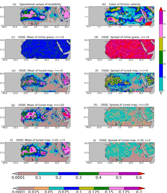
Fig. 1.Shows the mean and standard deviation of erodibility (α) map, except for(b). The vertical colorbar applies to(b). The upper
horizontal colorbar applies to the left column. The lower horizontal colorbar applies to the right column (except for(b)). The mean and standard deviations are those for the OSSE.(a)These operational values are used as the perfect values of erodibility (α) in the OSSE.(b)An index of the strength of friction velocity during June/July 2009. The color gives the fraction (expressed as percentage) of the total number (48) of times the friction velocity exceeds a value of 0.6 m s−1. For example, in the Horn of Africa the friction velocity is very strong, exceeding 0.6 m s−1at all times during the 48 cycles. See the vertical colorbar. The map ofu∗(not shown) looks different at each update cycle.(c)and(d): mean and standard deviation of the initial guess ofαmap, respectively, for the tuning experiment described in Sects. 3, 4 and 5.(e)and(f): mean and standard deviation of the map (after 48 update cycles), respectively, for the tuning experiment described in Sect. 4.(g)and(h): mean and standard deviation of the tunedαmap, respectively, for the tuning experiment with correlation length scale l=20 and cutoff radiusc=20 described in Sect. 5.(i)and(j): mean and standard deviation of the tunedαmap, respectively, for the tuning experiment with correlation length scalel=5 and cutoff radiusc=5 described in Sect. 5.
at 12:00 Z, 12 June 2009. The DA cycling frequency is 24 h. That is, the DA cycle (update) is implemented at 12:00 Z, every day. This frequency for update is chosen because real satellite data are available at 12:00 Z every day. The OSSE is run for 48 days, ending on 18 July 2009 at 12:00 Z, so that there are 48 update cycles. Only the AOD is observed. The
dust concentration and erodibility are not observed. In this work meteorological observations are not assimilated. The observational error is set to 10 % of the mean AOD observa-tion.
The forecasts did not improve with aerosol state estimation alone. The results from this experiment show that improv-ing the initial conditions in the dust concentration(cm)is not important. This is because the source and sinks of dust are strong over a 24 h period and play the key role in deciding the forecast. In other words, over a 24 h period the sources dominate the dust transport especially over areas of strong dust generation.
The theory underlying parameter estimation is the same as that of state estimation. Therefore, the state is augmented by the parameters (α) and data are assimilated. However, the dynamical equations to integrate the parameters in time for an untuned model are not known, which gives rise to some problems. The next section describes these problems and the methodology used in this work to address these problems. 3.1 Spread inα
The meteorological state variables (temperature, the three components of wind speed and humidity) have dynamics evolution equations that are used to integrate these variables forward in time between consecutive updates. However, in the imperfect model the parameterα(which is tuned in this work) does not have a dynamics evolution equation. At a par-ticular grid point we use the following equation to step for-ward each ensemble member ofαi,j
αijk (t+1)=αijk (t ) ,
wherekdenotes a particular ensemble member andtdenotes time. This is equivalent to using dα/dt=0 as the dynamical equation. If the trueα is constant in time, this equation is exact for a tuned system but is inexact for an untuned model. The dynamic evolution equation forα, used in this work, gives rise to another issue – that of spread inα. Theory of data assimilation states that each time data assimilation up-datesα, the spread inα must decrease or remain constant. The smaller the spread in α, the less impact observations in succeeding update cycles will have. Because dα/dt=0, the prior spread at a particular update is simply the posterior spread at the last update cycle. This problem is addressed in this work by using conditional inflation (Aksoy et al., 2006). If the posterior spread inαi,j falls below a particular
threshold value (1αt h), the posterior perturbations inαi,jare
scaled so that the spread is equal to a particular fixed value (1αfix).
αijk (t+1)=αijk (t )+1αfix
αijk (t )− ˜αij(t )
,
whereα˜i,jis the mean erodibility.
In this work the threshold value used is1αt h=0.05 and 1αfix=0.05. These values are chosen after experimentation with different values. If the mean of posteriorαi,j is close to
the limits ofαi,j (0 and 1), then a different strategy is
em-ployed. If the mean is less than 0.05 or more than 0.095, the
spread is set equal to 0.015. Also, if the posterior mean de-creases below 0.03 (inde-creases above 0.97) it is reset to 0.03 (0.97). One more issue is the risk of unphysical values of the posterior parameter ensemble. Negative values ofαi,jare
physically meaningless and it is possible that an update re-sults in negative values for some members of the posterior
αi,j. In this work such ensemble members with negative
val-ues are set equal to 0.01.
Before presenting the results of tuning over the whole do-main, in the next section the tuning ofαi,j (at a single grid
point) in the OSSE is explained. 3.2 Tuning at a grid point
It is instructive to consider the tuning of αi,j at a single
grid point, allowing the illumination of various issues in-volved in ensemble-based parameter estimation. The full three-dimensional COAMPS model is run with assimilation of simulated AOD data every 24 h. In the experiment de-scribed in this section the AOD is observed at all grid points. However, eachαi,j is updated using AOD observation only
at that grid pointi, j. This is because in this experiment the cutoff radius is set equal to zero (Hamill, et al., 2001).
The tuning ofαi,j at point K (Fig. 1a) as the update cycles
proceed is shown in Fig. 2a. It shows the mean and standard deviation of theαi,j estimate as the update cycles proceed.
The red line shows the truth; that is, the operational value of
αi,j at this point K. The mean and standard deviation of the
initial guess is 0.3 and 0.2, respectively. As the update cycles proceed the estimate ofαi,japproaches the correct value. For
this grid point, by 20 cycles the correct value is recovered. The estimates of AOD are shown in Fig. 2d.
In this example the αi,j update uses AOD observations
only at the same grid point, the mean of the posterior (or update) at any update cycle is given by
αup=αprior+ cov
(αprior,AODprior) var(AODprior)+var(AODobs)
AODobs−AODprior
. (3)
In this equation the subscripti, jis not used. All the quanti-ties in this equation are at grid point K. This equation is the Kalman equation for parameter estimation and is presented here to clarify the role of various quantities in the estimation. In this equation AODobs represents the AOD observation. The observational error variance is given by var(AODobs). The other terms are calculated from the short-term ensem-ble forecast (the prior). The covariance cov αprior,AODprior plays an important role in the update equation. This covari-ance exists because of the relation between AODprior and
α
eα
α
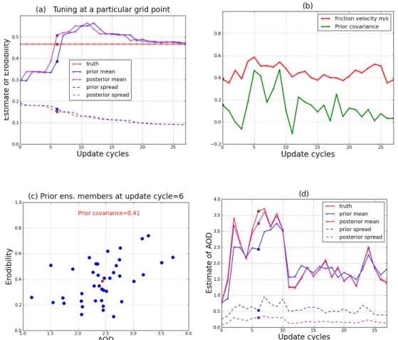
Fig. 2.Tuning of at a particular grid point marked K in Fig. 1a. The estimates of various quantities at this grid point are shown. See Sect. 3.2
for discussion.(a)Estimates ofα(means and spreads).(b)The time series of covariance betweenαand AOD is shown in green.(c)The prior ensemble members at update cycle 6. This update cycle is marked with squares in(a),(b)and(d). The red square shows the mean of the ensemble.(d)Estimates of AOD (means and spreads).
it advects dust from upstream regions. Therefore, the uncer-tainty in the AODpriorensemble is due to the uncertainties in localα, localu∗, upstreamα, upstreamu∗, and winds. From Eq. (2) the uncertainty in prior AOD can be written as Var AODprior=Var
AODlocalprior+VarAODtransportprior . (4) The contribution of uncertainty in local variables is contained in the first term on the right-hand side (rhs) of Eq. (4). The contribution from non-local variables and winds is given by the second term on the rhs of Eq. (4). Out of the total spread of AODprioronly a part is correlated with theαprior. This part is the first term of Eq. (4). The remaining spread is due to that in the transported AOD given by the second term that acts as advective additive noise. Given a particular magnitude of advective noise, the strength of the covariance between AODpriorandαpriordepends on the magnitude of the friction velocity. The time series ofu∗ and cov αprior,AODprioris shown in Fig. 2b. The covariance (scaled up by a factor of 10) is shown by the green curve. The covariance tends to be higher for higher values ofu∗. This is because stronger local generation helps the covariance signal to rise above
advec-tive noise. The prior AOD andαensembles at update cycle 6 are shown in Fig. 2c. The update cycle 6 is marked on each of the curves in Fig. 2a, b and d by squares. The red square in Fig. 2c shows the mean of the prior ensemble. The spread in the prior AOD ensemble in Fig. 2c includes spread due to localαand additive noise. A finite-size ensemble is used to estimate the true covariance. Because of the small size of the ensemble, it is expected that the ensemble estimate of covariances will not match the true covariance. Such covari-ances are termed spurious. Spurious covariance is basically an inaccurate estimate of the true covariance due to sampling errors. For example (Fig. 2b), the negative covariance val-ues at update cycle 4 and 11 are spurious. The finite (small) size of the ensemble (40 in this work) is the reason for these spurious covariances.
α
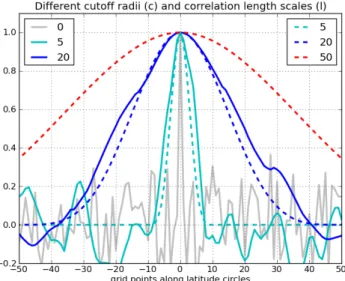
Fig. 3.Illustration of cutoff radius and correlation functions with
different length scales. The length scales are specified in units of grid points. The dashed lines show the Gaspari–Cohn localization functions with different cutoff length scales(c). The solid lines are correlation functions. For example, the solid blue line shows the correlation betweenαat the grid point marked 0 on the x-axis and the neighboring grid points forl=20.
locations are available and used in the estimation. In princi-ple,αat a single grid point is updated using all available ob-servations of AOD. The covariance betweenαand AOD at the observed grid point determines the weight given to the in-novation in the calculation of the increment. This covariance is calculated using the ensemble. If a very large ensemble size is used, the ensemble covariance is more accurate. With a small ensemble size the estimated covariance tends to be in-accurate, especially if the true covariance is small. The true covariance with a grid point geographically far away tends to be smaller, and hence the estimated covariance should be trusted less for far away grid points. The concept of a cutoff radius or a localization radius is widely used in ensemble-based filtering work to address the problem of spurious co-variances (Hamill, et al., 2001). The cutoff radius,c, dictates the distance over which observations are used to calculate the correction. This is achieved by defining a (localization) func-tion that decays as one moves away from the grid point being tuned. The Gaspari–Cohn function (Gaspari and Cohn, 1999) is used in this work. The width of this function is governed by the value ofc. In the current work, we will run experiments with various values ofc. The functions corresponding to the values ofcused in this work are shown in Fig. 3 as dashed curves for a single grid point. This grid point is marked 0 on the x-axis. The dashed cyan curve shows the Gaspari–Cohn function corresponding toc= 5 grid points. In this work the distance is mentioned in units of grid points. The horizontal resolution used in this work is 81 km (5 grid points is equal to 400 km).
The functions peak at the grid point marked 0. This is the grid point whereαis being tuned. The Gaspari–Cohn func-tion value at a particular grid point is used as a multiplicative factor to decrease the weight given to the observation in cor-recting theαat that grid point. The functions are shown in one dimension along a latitude circle in Fig. 3. However, ac-tual functions are defined in two dimensions. Practically, ob-servations at all grid points more than a distance of 2cfrom the point of interest do not have any impact on the correc-tions.
In the next section the results of tuningα(all over the do-main) is described.
4 Tuning with uncorrelatedαperturbations in OSSE
In the last section it was assumed that observations of AOD are available at all points in the domain, whereas in reality ac-tual satellite observations are available for many (but not all) locations. At any given update cycle the satellite observations are sparse. This sparseness of satellite observations is mim-icked in the OSSE by observing AOD at 20 % of grid points in the domain. These 20 % grid points are randomly chosen at each update cycle. In the satellite observations, however, the sparse regions need not change randomly with time. The observational error is set equal to 10 % of the mean AOD observation. This observational error is motivated by AOD satellite data whose error is at least 10 % of mean observa-tion.
We begin with an experiment in which the cutoff radius is set to zero. This means thatαi,j at any given grid point uses
only the AOD observation at that grid point. The mean and standard deviation of the initial guessαis shown in Fig. 1c, d. The perturbations inαin initial guess are uncorrelated. The result of this experiment; that is, the ensemble mean of the tunedα(after 48 cycles) over the domain is shown in Fig. 1e. The uncertainty in this estimated mean is given by the stan-dard deviation in the ensemble which is shown in Fig. 1f. Be-cause this experiment is an OSSE we know the perfect values of erodibility at every grid point which is shown in Fig. 1a.
ints. Th
Fig. 4.Yellow color points show the (correctly) tuned grid points.
The white or clear grid points show the untuned points. The (cor-rectly) tuned point lies within 0.05 absolute units of the perfect value at a given grid point. The blue colored contours enclose areas with strong friction velocity (Fig. 1b) . The red contours enclose ar-eas with high erodibility (Fig. 1a).(a)Shows the quality of tuning for the tuning experiment corresponding to Fig. 1e.(b)Shows the quality of tuning for the tuning experiment corresponding to Fig. 1i.
The success of the tuning experiment is further quanti-fied by comparing the tunedα value at each grid point to the true α value at that grid point. α at a particular grid point is deemed to be (correctly) tuned if its tuned value lies within 0.05 of the true value at that grid point. Other-wise it is deemed to be untuned. This criterion of 0.05 (in absolute units ofα) is an arbitrary choice. This criterion is used throughout this work to determine the quality of tun-ing. The distribution of the tuned and untuned points over the domain is shown in Fig. 4a. The grid points colored with yellow are those tuned successfully. The white grid points are the untuned grid points. The blue contours enclose ar-eas with high friction velocity. These contours correspond to areas in which the friction velocity is above 0.6 m s−1at least 20 % of times (Fig. 1b). The red contours enclose areas with high true erodibility (more than 0.25). Some of the areas with high friction velocity are marked S1, S2 and S3. Notice that in these areas the tuning is successful. In the Horn of Africa (S1) almost all the grid points are successfully tuned. Recall that the friction velocity gives rise to the covariance signal. Consequently areas with strong friction velocity tend to be tuned well. Some areas with weak friction velocity are marked W1, W2, W3 and W4. These areas tend to be poorly tuned. Consider area W1. Note that W1 is an area of weak friction velocity sandwiched between areas of high friction velocity on its north and south. Not only does it have a weak signal but also high advection noise because it lies in an area of high erodibility (it is enclosed by the red contour). As pointed out in Sect. 3.2, the advection noise is additive noise. The combination of low friction velocity (small local signal
l
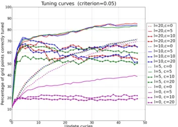
Fig. 5.The tuning curves for OSSE experiments with different
val-ues oflandc. Each curve shows the percentage of grid points tuned correctly as the update cycles proceed. The values ofl andcare specified in grid point units. A distance of 10 grid points corre-sponds to 800 km. For this problem a correlation length scale of 5 grid points (400 km) gives the best results. See Sects. 4 and 5 for discussion.
of AOD), and large amounts of advected AOD makes it diffi-cult to correctly estimate the erodibility parameters. The sit-uation is similar with area W3 in the Arabian Peninsula and W2 in the center of the domain. The area W4 in the south of the Sahara has weak friction velocity and low erodibility.
Using this criterion of 0.05, the number of grid points suc-cessfully tuned is counted and expressed as percentage of the total number of grid points. This percentage is shown in Fig. 5 as the dashed magenta curve. By the end of 48 update cycles, about 70 % of the points in the domain are correctly tuned.
with many observations, the update uses many bad covari-ances. The reason for the bad covariances is a combination of the effect of advective noise and the small size of the en-semble. The covariance betweenαat a particular point and AOD at another point is partly controlled by the correlation betweenαperturbations at these two points. For the exper-iment described in this section, the updates do not result in correlating theα perturbations; that is, the initially uncor-relatedαperturbations remain uncorrelated at the end of all the update cycles. In the current experiment the perturbations are uncorrelated, and hence dust generated by all the points within the neighborhood of point of interest contributes to the advective noise. The small ensemble finds it difficult to capture the local signal due to this advective noise resulting in spurious covariances. Hence, including the observations of AOD from neighboring grid points degrades the tuning rather than improving it. The solid magenta curve shows the result of the experiment withc= 5. Its performance is intermediate betweenc= 0 and c= 20. The experiment withc= 10 (ma-genta circles) gives almost the same result as that withc= 20. However, one would like to use as many observations as possible by settingc >0. The main hurdle to usingc >0 is the advective noise. What can be done to address this prob-lem? A possible solution to this problem is to correlate the perturbations in neighboringα, thereby reducing the advec-tive noise. Also, the results of the experiments in this section suggest that the assimilation of observations does not impose a correlation structure in theα field. That is, the observa-tions are unable to recover the correlation structure (if any) between initially uncorrelatedα. Can the assimilation of ob-servations recover the correlation structure if theα perturba-tions are initially correlated? The next section considers the issue of initially correlatedαperturbations.
5 Tuning with correlatedαperturbations in OSSE
In this section the initial perturbations ofαare spatially cor-related. Some examples of the correlation functions between theα perturbations are shown in Fig. 3. The point marked 0 on the x-axis is the point of interest. The solid blue curve gives the correlation between theαperturbations at point 0 and that at various neighboring points along the latitude cir-cle corresponding to a correlation length scale ofl=20 grid points. The standard deviation of this correlation function isl=20. This correlation is constructed by first sampling from (uncorrelated) ξ (0.25,0.25) and then constructing a spatially smoothed perturbation for each ensemble member separately. These weights are chosen proportional to a two-dimensional Gaussian function with standard deviation of
l=20. The cyan curve shows the correlation function for
l= 5. The gray curve shows the correlation function forl=0; that is, independent perturbations. The correlation function of any grid point in the experiment described in the Sect. 4 looks like the gray curve. The termcorrelation functionwill
imply correlations between α perturbations (between two grid points).
The red (squares) curve in Fig. 5 shows the tuning curve for an experiment with correlation length scalel=20 and cutoff radiusc=20. The initial mean and standard deviation for this experiment is shown in Fig. 1c and 1d, which is the same as that for the l=0 experiment described in Sect. 4. The initial guess for the magenta curves and red (squares) curve in Fig. 5 is the same, except that for the red curve the initialαperturbations are correlated over a length scale of 20 grid points. The correlation function of any grid point in the domain forl=c=20 experiment looks like the solid blue curve in Fig. 3. The red (squares) curve in Fig. 5 shows that the tuning is successful for about the first 5 update cycles and there after degrades. The reason for this degradation can be understood by considering the correlation function at a particular grid point as the update cycles proceed. The cor-relation function at a particular grid point (marked x in area W1 in Fig. 4) is shown in Fig. 6 as the solid green curve. The number in each panel indicates the update cycle. At the ini-tial time a correlation length scale ofl=20 is imposed. The green curve is the correlation between theαperturbations at the point marked 0 on the x-axis and that at the neighbor-ing grid points around the latitude circle. The dashed yellow line shows the localization function corresponding to cutoff radiusc=20. The dashed black curve in each panel shows a Gaussian with length scale of 5 grid point for reference. At each update cycle AOD data are assimilated and all these αperturbations are updated, thereby modifying the correla-tion ofαwith surrounding points. As the update cycles pro-ceed, the correlation function narrows down, as seen in the successive panels in Fig. 6. In fact, it converges towards a function with a length scale of about 5 grid points as seen in the last few update cycles. The parameter estimation re-sults in a length scale ofαperturbations of approximately 5 grid points, but the localization is allowing information from much further away to impact the local estimate ofα. The cor-relations with points further away than 5 grid points tend to be bad, and hence as the updates proceed the red (squares) curve in Fig. 5 degrades.
The correlation functions for many grid points at various locations are inspected, and it is found that the correlation length converges to about 5 grid points. A new tuning exper-iment is run withl=5,c=5. The result of this experiment is shown in Fig. 5 as the solid green curve. Clearly,l=5,
c=5 performs far better thanl=c=0 andl=c=20. An-other experiment is run withl=20,c=5. The tuning curve for this experiment is shown by the solid red curve in Fig. 5. The tuning for l=20, c=5 is as good as that for l=5,
ked
Fig. 6.Evolution of the correlation function at a particular grid point (marked x in area W1 in Fig. 4) for the experiment withl=c=20.
Each panel is for a different update cycle. The numbers inside each panel show the update cycle.
The tuned map at the last update cycle forl=20,c=5 experiment is shown in Fig. 1i. The tuned map correspond-ing to thel=c=20 experiment (solid red (squares) curve in Fig. 5) is shown in Fig. 1g. Clearly, the tuned map in Fig. 1i recovers the perfect map shown in Fig. 1a more accurately than does thel=c=0 experiment (Fig. 1e) or thel=c=20 experiment (Fig. 1g). Comparing Fig. 1f and Fig. 1j the estimate from thel=20,c=5 experiment is con-strained better thanl=c=0 experiment as can be inferred from the lower values of spread in Fig. 1j.
The spatial distribution of tuned points forl=20,c=5 experiment is shown in Fig. 4b. Comparing this figure with Fig. 4a correlating perturbations and using more observations leads to tuning gains in high advection/low friction velocity regions like W1, W2, W3 and W4. This strengthens, to some extent, our hypothesis that correlating perturbations leads to an improvement in the covariance estimates. This improve-ment in the signal (covariance) can be considered to be an
effectivedecrease in advection noise. The reduction in the degrees of freedom (because of correlations) increases the impact of observations, thereby improving the tuning. It ap-pears that for this particular problem, on an average over the domain, an emergent correlation length scale is about 5 grid points (400 km). Imposing a correlation function ofl=5 is leading to better covariances. This does not mean that ad-vection mainly happens over a length scale of 5 grid points. Advection most probably is taking place over longer length
d c at
Fig. 7.Comparison between tuning for different values oflandcat
a particular point. This point is marked x in the W1 area in Fig. 4. The evolution of the correlation function at this point is shown in Fig. 6.
scale. However, the linear signal due to advection survives only over a length scale ofl=5 grid points.
Various other experiments with different values ofl and
c are run to further investigate the interplay between cor-relation length and cutoff radius. The red and blue curves correspond to experiments with correlation length scalesl=
(squares) curve. Forl=20,c=10, the correlation function narrows down and converges to about 5 grid points, similar to the case ofl=c=20. However, the degradation is not as much as thel=c=20 because only observations within ra-dius ofc=10 grid points are being assimilated. The amount of bad covariances being used is less in the c=10 exper-iment compared to the c=20 experiment. The experiment withl=10,c=5 (solid green curve) gives a result compa-rable withl=5,c=5 andl=20,c=5. This shows that if
l > c, then the correlation length is effectivelyl=cas far as the data assimilation is concerned. As the update cycles pro-ceed,l converges to 5 grid points. Before this convergence happens sincec < l, the observational information beyond a distance ofc is not used. For thel=10 experiments with
c=10 (blue circles) andc=20 (blue squares), the behavior is similar to thel=20 experiment with similar values of c. This shows thatl >5 is too broad for this problem and ifc
is specified longer than 5, then the data assimilation narrows the correlation function to 5 grid points. Lastly, consider the dashed curves that show results forc=0 for various values of l. These curves approximately overlap, showing that it is futile to correlate perturbations without using observations in the neighborhood. The curves withc >=l, forc >5, show that using observations outside the correlated area degrades the tuning, which is because of inaccurate covariances. Fig-ure 7 shows the tuning at a particular point marked x in W1 area Fig. 4. The dashed magenta line uses observations only at the same grid point, and hence the updates take place only when data are available at that grid point. Though the solid magenta curve has access to more observations, the covari-ance estimates are not good enough because the perturbations are not correlated. The red curve (squares) uses observations over a length scale ofc=20, while as the updates progress the correlation narrows to 5 grid points. Consequently, the estimate does not converge towards the perfect value ofαat this grid point very well. The solid green, blue and red curves converge smoothly because the correlation is over a scale of 5 grid points. These curves have access to more observational information and improved signal because of correlation.
The results from all these experiments suggest that the ob-servations are able to uncover the correlation scale between neighboringαfield, provided the initialαperturbations are correlated over a broad length scale. This correlation scale for this problem is about 5 grid points. As seen in Sect. 4, if the initialαperturbations are uncorrelated, the observations are not able to impose a correlation structure as the updates proceed.
The sensitivity of the OSSE tuning results to ensemble size was found by running experiments with smaller ensem-ble sizes. As noted, for an ensemensem-ble size ofN=40, about 85 % of the grid points are tuned for thel=20,c=5 exper-iment (solid red curve in Fig. 5). This percentage decreases to 75 %, 60 % and 45 % for an ensemble size of 20, 10 and 5, respectively.
Though results from the OSSE experiments are not guar-anteed to hold for experiments with real data, they do provide valuable insights into the tuning of erodibility. They show that under ideal circumstances the erodibility is amenable to tuning, given realistic observational coverage and errors. Ideal circumstances mean that the only model error is im-perfect values of erodibility. Even so it provides confidence in the tuning methodology to proceed with experiments with real data. The next section describes the tuning experiments with real satellite data.
6 Real data
In this section the tuning experiments with satellite data are described in Sect. 6.1. In Sect. 6.2 the estimated map of erodibility is verified using satellite data.
6.1 Tuning
MODIS Deep Blue data (Remer et al., 2005; Hsu et al., 2004, 2006; Shi et al., 2011) are used for the experiments with real data. The satellite data are averaged over a box of 3 grid points (about 240 km) to obtain super observations. The er-rors in the observations could be correlated. The averaging serves to decorrelate these errors. The super observations are assimilated into the COAMPS model using the ensemble-based tuning methodology. Here the observational error is set equal to 0.15 + 10 % AOD units, but realistically the er-rors for some locations can be considerably greater (Shi et al., 2011). Shi et al. (2011) also found that lower values of AOD observations tend to have higher relative uncertainty than higher values. Incorporating 0.15 AOD units in the ob-servational error assigns high errors to observations below 0.15. The tuning experiment for the real data runs from 12 June 2009 to 8 July 2009. MODIS satellite data are assim-ilated every 24 h at 12:00 Z. In total the tuning experiment uses 28 update cycles. The period from 8 July 2009 to 30 July 2009 is used for verification. The threshold friction ve-locity is set to 0.6 m s. It has to be noted that the experiment with real data is completely separate from the OSSE experi-ment described in Sects. 3, 4 and 5.
s
α
α
Fig. 8.The tuning experiment with real satellite data. The left colorbar is for(a)and(c). The right colorbar is for the standard deviations
shown in(c)and(d).(a)The operational values ofαare used as mean of initial guess.(b)Standard deviation of initial guessαare is set equal to 0.25.(c)The mean of tuned values after 28 update cycles.(d)The standard deviation of tuned values after 28 updates cycles.
in Fig. 8c. The standard deviation in the mean of these tuned values is shown in Fig. 8d.
The estimates ofα as a function of the update cycles at four different grid points is shown in Fig. 9. For the grid point in panel (a) the estimate decreases from 0.3 to about 0.05. The convergence is not smooth, but clearly the esti-mation corrects a bias in the first guess in the downward direction. Between cycles 10 and 28 the mean wiggles be-tween 0.05 and 0.1 rather than staying at a constant value. This is because the estimated erodibility can compensate for other errors in the model like those in threshold velocity and advection. Similarly in panel (b) the estimation corrects the erodibility in an upward direction but does not remain con-stant. Panel (c) shows a case where the erodibility has clearly not converged. In panel (d) the estimate appears to converge between updates 10 and 15, but undergoes large variation af-ter update 20. The estimation curves shown in these panels are representative of many locations in the domain. The as-sumption that the model is imperfect only in the erodibility is too simplistic. There are many other imperfections in the model. The estimate of erodibility inadvertently corrects for these imperfections. The imperfections in threshold velocity and near surface wind would have the highest impact on the estimate of erodibility because these control the dust flux. The friction velocity depends on the 10 m wind. It is possible that the estimation correctsαto account for imperfection in the 10 m wind. Therefore, one has to exercise caution while interpreting the tuned map of erodibility.
Considering the tuned map (Fig. 8c), on an average in the west Sahara and the Arabian Peninsula the parameter estima-tion results in lower values ofαcompared to the operational values (Fig. 1a). It is possible that the estimation decreases the erodibility in these areas to correct for a positive bias in the friction velocity. In the south Sahara region (between lat-itude 5 and 10◦N)α converge to higher values. During the tuning process the ocean values ofα are set equal to zero
t 4
Fig. 9.Each panel shows the mean and spread of the erodibility at
4 different grid points for the real data experiment. The latitude and longitude of the point is mentioned in the title of each panel.
within the model. Comparing (Fig. 8) panel (b) and (d) it is evident that the standard deviation in the mean of the tuned values decreases to about 0.05 compared to the initial guess standard deviation.
Since one does not know the real erodibility, the tuned map has to be assessed indirectly by verifying forecasts of AOD. The next section describes such a verification experiment. 6.2 Verification
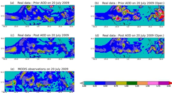
Fig. 10.Mean AOD estimates on 20 July 2009 at 12:00 Z.(a)and(b): priors using the tuned (Fig. 8c) and the operational maps (Fig. 1a),
respectively.(c)and(d): posteriors obtained by assimilating satellite data into the priors shown in(a)and(b), respectively.(e)Satellite data.
8 July 2009 to 30 July 2009 (19 days) is used for verification. Two separate data assimilation (verification) experiments are run over the verification period. In these experiments only the dust concentration and AOD fields are estimated. The erodi-bility parameter map is held fixed. The first DA experiment uses the operational erodibility map (Fig. 1a) and the second uses the tuned erodibility map (Fig. 8c). The same MODIS observations are assimilated in each of these experiments. For each experiment we have access to analysis ensemble on 19 different days. For each experiment, 24, 48, 72 and 96 h ensemble forecast is launched from each of these analy-sis ensembles. Consequently, for each of the two experiments we have 19 different forecast ensemble means. The MODIS observations at the respective days are used to verify the fore-cast means in each experiment. For a given day MODIS ob-servations are used to verify the forecast launched from the last day, but this data are also assimilated to generate the pos-terior. This is not a problem because 24 h is long enough for the dust generation and transport to render the forecast almost independent of the initial conditions. The source of dust, that is the erodibility values, plays a dominating role in deciding the spatial distribution of dust over the 24 h period. Consider the verifications of these two experiments on a particular day. Figure 10 shows the mean estimates of AOD on 20 July, 2009. Panel (e) shows the satellite observations of AOD at 12:00Z, 20 July 2009. The right side panels ((b) and (d)) corresponds to the operational experiments. Panel (a) and (c) shows the estimates from the tuned experiment. The same MODIS data are assimilated into each of these ex-periments. The prior shown in panel (a) is the mean of the 24 h ensemble forecast launched starting from the posterior AOD on 19 July 2009 for the tuned experiment. This fore-cast for the operational experiment is shown in panel (b).
Comparing panel (a) and (b) to (e), the tuned forecast agrees with the observations more than the operational forecasts. Panel (c) shows the posterior AOD field corresponding to the prior in panel (a). Panel (d) shows the posterior corre-sponding to panel (b). The same data (panel (e)) are assimi-lated into the tuned and operational priors to obtain posteri-ors in panels (c) and (d), and hence these posteriposteri-ors are sim-ilar. These posteriors are used as initial conditions to launch the next 24 h ensemble forecasts. These forecasts (priors) valid at 12:00 Z, 21 July are shown in panels (a) and (b) in Fig. 11. The satellite observations on 21 July 2009 are shown in Fig. 11c. The tuned forecast (panel (a)) matches better with the observations (panel (c)) than does the operational forecast (panel (b)). Note that these tuned and operational forecasts used similar initial conditions in AOD, which are given by panel (c) and (d) of Fig. 10. In spite of these similar initial conditions, the operational forecast (prior) is different from the tuned forecast on 21 July with operational forecasts giving higher AOD values on 21 July. Note that the same meteorology is used in both the operational and tuned ex-periments. The only difference between the tuned and opera-tional experiments is the different maps of erodibility. There-fore, the difference between these forecasts is due to different values in the erodibility maps. The lower values of AOD in tuned forecasts are attributable to lower values of erodibility in the tuned map (Fig. 8c) compared to the operational map (Fig. 1a).
rbar
Fig. 11.Mean AOD estimates on 21 July 2009 at 12:00 Z. See the colorbar in Fig. 10.(a)and(b)are the forecasts launched from the tuned
and operational posteriors on 20 July, respectively.(c)Satellite data.
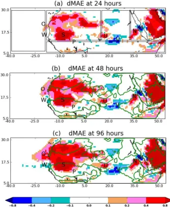
Fig. 12.Result of the verification experiment. The green contours
enclose areas of strong friction velocity.
the mean operational forecast and the MODIS observation is calculated.
ε0=AODop−AODobs
Then at each grid point, the average ofε0over different fore-casts is the mean absolute error for the operational model. Similarly, the absolute difference between the mean tuned forecast (AODtu)and observation is calculated.
εtu= |AODtu−AODobs|
Figure
Fig. 13.AOD verifications at grid points S and P in Fig. 12. Legend
in(b)applies to(a).
At each grid point, the average ofεtuover different forecasts is the mean absolute error for the tuned model. At each grid point, the operational and tuned mean absolute errors are used to calculate the metricdifference mean absolute error
Fig. 14. The scatter plots of forecast AOD (24 h lead time) and AOD observations.(a)corresponds to the box containing point S in Fig. 12a.(b)corresponds to the box containing point U in Fig. 12a. (c)corresponds to the box containing point N in Fig. 12a.
dMAE=εop−εtu
This metric is a simple and convenient way to quantify the comparative performance of the operational and tuned mod-els in forecasting the AOD, at each grid point. If dMAE>0 it means that the operational model errs more than the tuned
model in forecasting the AOD. If dMAE>0 at a particular grid point, then the tuned model outperforms the operational model. On the other hand, if dMAE<0 it means that the op-erational map performs better at that grid point.
The dMAE corresponding to the tuned map in Fig. 8c is shown in Fig. 12, with contours of high friction velocity over-laid. Figure 12a shows the dMAE calculated for the forecast lead time of 24 h. The tuned map outperforms the operational map largely in the west Sahara and Arabian Peninsula re-gions. The tuned map gives better forecasts than the opera-tional map to some extent in the Horn of Africa. In most of the other regions the dMAE is within−0.1 and+0.1, indi-cating that the tuned and operational forecast are almost sim-ilar. There are a couple of pockets near central Sahara where the tuned map gives degraded performance. These areas are blue in color. Panels (b) and (c) in Fig. 12 show the dMAE for longer lead times of 48 and 96 h, respectively. Compar-ing panels (a), (b) and (c) it is clear that broadly the pattern of areas where the tuned model outperforms the operational model are similar for all lead times. However, comparing the red areas in the vicinity of point S in panels (a) and (b) the tuned model performs better over a larger region for the 96 h forecast compared to the 24 h forecast. Also, the magnitude of improvement of the tuned model is higher for longer lead time in this area. This is also true in the Arabian Peninsula. An important dMAE feature that develops with longer lead times is in the vicinity of points O and W off the coast of Africa. The red color near point O in panel (c) indicates that the tuned model gives a better forecast at 96 h, whereas the tuned model is as good as the operational model in this area at 24 h. In Fig. 13 the relative performance of the tuned and operational models is further probed by inspecting the AOD forecasts at two of the points marked in Fig. 12.
The time series of AOD forecasts at point S are shown in Fig. 13a. The black curve shows the AOD observations. The dashed green curve showsu∗ scaled by a factor of 5, dur-ing the verification period. Clearly,u∗is above the threshold level of 0.6 m s for almost all the verification times. The solid curves show the operational forecasts at lead times of 24 and 96 h. The dashed curves show the tuned forecasts. The title of the panel shows the value of operational and tuned erodi-bility. At point S the operationalαis 0.32 and the tunedαis 0.04. The title of the panel also shows the dMAE at 24 and 96 h, which is 2.2 and 2.9, respectively. The number 78.0 and 95.0 shown in the panel are the percentage of times when the
u∗ exceeds the threshold value during the tuning and veri-fication periods, respectively. So at this point out of the to-tal number of cycles (28) in the tuning period,u∗ exceeds the threshold value 78 % of times. This point is an example of a grid point whereu∗is very strong both during the tun-ing and verification periods. Because the signal is strong dur-ing the tundur-ing period, this point istuned correctly, decreas-ing the value from 0.32 to 0.04. The phrasetuned correctly
the conclusion that the tuned value is correct. The dashed blue curve matches well with the observations while the op-erational forecast (blue curve) is too high. The low value of tuned AOD can be directly attributed to the lower value of tuned erodibility at point S. Note that the tuned AOD not only has a smaller bias (with respect to the observations) com-pared to the operational AOD values but also a smaller stan-dard deviation. In both the tuned and operational model the 96 h forecast is higher than the 24 h forecast. This suggests that there is some accumulation of dust over the 96 h. This accumulation seems to be more for the operational than the tuned model as the separation between red and blue curves is larger for the operational model. This accumulation might be because in the operational model the production is more because of higher erodibility of 0.32 (compared to 0.04). The higher dMAE of 2.9 at 96 h compared to 2.2 at 24 h means that the operational model errs more (compared to the tuned model) at 96 h than at 24 h. Note that both the operational and tuned forecasts follow the variations in the friction velocity (green curve).
In Fig. 12 consider the white area to the lower right of point S, around the point marked P. The verification for this point is shown in Fig. 13b. At this point, u∗ exceeds the threshold value for about half the time during both tuning (60 %) and verification (55 %) periods. This point has low value of erodibility in the operational map. Because the op-erational values arecorrectthe tuning methodology does not change this value much. The inference that these values are
correctis drawn from the fact that at point P both operational and tuned models do (equally) well in predicting the obser-vations.
The inspection of the forecasts’ time series and observa-tions shown in Fig. 13 suggests that the positive dMAE in Fig. 12 is because the tuned model AOD has a lower bias compared to the operational model AOD.
The biases in the tuned and operational models for vari-ous regions are shown in Fig. 14. These varivari-ous regions are marked by boxes in Fig. 12a. The panel (a) shows the scat-ter plot of AOD observations versus the forecast AOD in the west Sahara region. The red dots show the operational AOD. The grey line is a reference line with zero bias and slope equal to unity. The red line is the linear fit to the red dots. This linear fit is given by the equation AODop=a×AODobs+b
The regression coefficientsaandb(which is the bias) are shown in the upper right corner of the panel. The blue line is the linear fit to the cyan dots, which shows the tuned AOD. The tuned model reduces the bias from 0.56 to 0.31. Though the tuned model on an average overestimates the AOD by 0.31 it decreases the bias by 0.25 (compared to the opera-tional model) which is a substantial improvement.
The panel (b) shows the scatter plot for the east Saharan re-gion. In this region the tuned model increases the bias (0.12). The operational model has a small negative bias of−0.04.
0.46 from 0.72 to 0.26 in the Arabian Peninsula.
The decrease in bias in the west Sahara and the Arabian Peninsula contributes towards the positive dMAE in these regions. This decrease in bias is due to the downward cor-rection of the tuned erodibility values (compared to the oper-ational values) in these regions. In the south Saharan region the operational bias is−0.09 (result not shown). The tuned model changes this bias to 0.07. This might be due to upward correction in tuned values in the south Saharan region. The positive bias of 0.12 in the east Saharan region might be due to the increased advection from the south Saharan region. In the Atlantic region the biases in the tuned and operational model are comparable (results not shown).
Consider Fig. 12c. The red areas coincide with areas with high operational erodibility. In these areas (west Sahara and the Arabian Peninsula) the operationalα was corrected by the tuning to a lower value. In the (white) areas other than west Sahara and the Arabian Peninsula, both operational and tuned maps perform equally well. The improvement of fore-casts in west Sahara and the Arabian Peninsula is because tuning leads to a better model of dust generation by decreas-ing the erodibility. However, an improvement in the dust gen-eration over the red areas does not impact the forecasts in the other areas. This means that the effect of tuning is local-ized in space. This might be because of the model error in dust transport. Both the tuned and operational models used the same meteorology and therefore the same winds. These might be different from the winds in nature. Both the tuned and operational model suffer from the model error in meteo-rology. Because of this model error in dust transport, the im-proved dust generation in the red areas might not necessarily improve dust forecasts in other areas. In this work meteoro-logical variables are not estimated.
At almost all the points in the domain (two of which are shown in Fig. 13), the 96 h forecasts are higher than the 24 h forecasts, for the tuned and the operational model separately. The higher AOD at longer lead time points to accumula-tion of AOD either from local producaccumula-tion or from upstream transport. The higher AOD at 96 h explains the larger cov-erage of the red area in the Sahara in Fig. 12c compared to Fig. 12a. Because both the models use the same meteorology and sinks, the higher operational AOD at 96 h is due to higher production in the upstream areas. This higher production is due to the higher operational erodibility.
The tuned and operational forecasts were compared to cli-matology, and it was found that neither were able to outper-form the climatology.
7 Conclusions and further work