www.atmos-meas-tech.net/6/1747/2013/ doi:10.5194/amt-6-1747-2013
© Author(s) 2013. CC Attribution 3.0 License.
Atmospheric
Measurement
Techniques
Geoscientiic
Geoscientiic
Geoscientiic
Geoscientiic
MODIS 3 km aerosol product: applications over land in an
urban/suburban region
L. A. Munchak1,2, R. C. Levy1, S. Mattoo1,2, L. A. Remer3, B. N. Holben1, J. S. Schafer1, C. A. Hostetler4, and R. A. Ferrare4
1Earth Science Division, NASA Goddard Space Flight Center, Greenbelt, MD 20771, USA 2Science Systems and Applications, Inc., Lanham, MD 20709, USA
3Joint Center for Earth Systems Technology (JCET), University of Maryland Baltimore County, Baltimore MD, 21228, USA 4NASA Langley Research Center, Hampton, VA 23681, USA
Correspondence to:L. A. Munchak (leigh.a.munchak@nasa.gov)
Received: 31 January 2013 – Published in Atmos. Meas. Tech. Discuss.: 14 February 2013 Revised: 14 June 2013 – Accepted: 17 June 2013 – Published: 23 July 2013
Abstract.MODerate resolution Imaging Spectroradiometer (MODIS) instruments aboard the Terra and Aqua satellites have provided a rich dataset of aerosol information at a 10 km spatial scale. Although originally intended for climate appli-cations, the air quality community quickly became interested in using the MODIS aerosol data. However, 10 km resolution is not sufficient to resolve local scale aerosol features. With this in mind, MODIS Collection 6 includes a global aerosol product with a 3 km resolution. Here, we evaluate the 3 km product over the Baltimore–Washington D.C., USA, corri-dor during the summer of 2011 by comparing with spatially dense aerosol data measured by airborne High Spectral Res-olution Lidar (HSRL) and a network of 44 sun photometers (SP) spaced approximately 10 km apart, collected as part of the DISCOVER-AQ field campaign. The HSRL instrument shows that AOD can vary by over 0.2 within a single 10 km MODIS pixel, meaning that higher resolution satellite re-trievals may help to better characterize aerosol spatial dis-tributions in this region. Different techniques for validating a high-resolution aerosol product against SP measurements are considered. Although the 10 km product is more statistically reliable than the 3 km product, the 3 km product still per-forms acceptably with nearly two-thirds of MODIS/SP col-locations falling within an expected error envelope with high correlation (R >0.90), although with a high bias of∼0.06. The 3 km product can better resolve aerosol gradients and retrieve closer to clouds and shorelines than the 10 km prod-uct, but tends to show more noise, especially in urban ar-eas. This urban degradation is quantified using ancillary land
cover data. Overall, we show that the MODIS 3 km product adds new information to the existing set of satellite derived aerosol products and validates well over the region, but due to noise and problems in urban areas, should be treated with some degree of caution.
1 Introduction
air quality conditions (e.g. Hutchison, 2003; Wang and Christopher, 2003; Chu et al., 2003; Engels-Cox et al., 2004; Hutchison et al., 2004). The MODIS instruments are particu-larly appealing for air quality applications because the broad (2330 km) swath of the instrument allows most global loca-tions to be monitored on a nearly daily basis. However, the 10 km resolution of the MODIS aerosol products is insuffi-cient to resolve small-scale aerosol features, including point sources in urban areas (C. C. Li et al., 2005) and small fire plumes (Lyapustin et al., 2011). Although several research techniques exist to retrieve aerosols at higher spatial scales (100 m to 1 km) from MODIS observations (e.g. Lyapustin et al., 2011; Li et al., 2012), these have not been produced globally in an operational environment.
In response to clear scientific needs for aerosol observa-tions at a higher spatial resolution, MODIS Collection 6 will include a global aerosol product at nominal 3 km scale, in addition to the standard 10 km resolution. This 3 km product will include retrievals based on both dark target algorithms (land and ocean). Remer et al. (2013), describe the 3 km product in detail, and analyze a six-month test database to compare the performance of the 3 km and 10 km products on a global scale. The 3 km product can show more spatial de-tail than the 10 km product, but agrees less well with ground-based sun photometers on a global scale. However, the 3 km product may be better at characterizing aerosol distributions on local scales, and can only be tested through comparison with dense observations on a small spatial scale. We wish to examine the 3 km aerosol product on a regional scale to determine the additional information content that the higher resolution retrieval provides, and the possible degradation in data quality introduced by moving to a higher resolution.
In this work, we focus primarily on AOD, because it has been used for surface air quality applications (van Donkelaar et al., 2006) and can easily be compared with lidar and sun photometer data. Specifically, we can evaluate AOD prod-ucts at both 10 km and 3 km resolutions by comparing with surface- and airborne-based AOD measurements collected during the DISCOVER-AQ field campaign conducted during the summer of 2011 over the Baltimore–Washington D.C. corridor of the United States. We first assess the similarities and differences in 10 km and 3 km MODIS AOD images, and evaluate whether the 3 km product provides information that is not captured by the 10 km product. We look critically at the best method to validate the higher resolution aerosol re-trieval against sun photometer measurements, and validate the 10 km and 3 km products for the campaign duration. The ability of the MODIS product at both 10 km and 3 km resolu-tions to capture spatial variability in AOD is also addressed. Due to the limited validation data for the over ocean vari-ables, we will only address the land variables in this study.
2 The MODIS 3 km land algorithm
The retrieval method of the global MODIS 3 km aerosol product is thoroughly detailed in Remer et al. (2013). For the sake of completeness, we will briefly describe the land algorithm here. The 3 km algorithm emerges from the “dark target” retrieval methodology (Kaufman et al., 1997a; Tanr´e et al., 1997; Remer et al., 2005; Levy et al., 2007b, 2013), based on the concept that in the visible wavelengths, aerosols are bright and vegetated surfaces tend to be dark. The spec-tral contrast between aerosols and the surface can be used to retrieve quantitative information about aerosol properties.
To increase signal-to-noise, the MODIS algorithm re-trieves aerosol parameters at a lower spatial resolution than the nominal (at nadir) 500 m top of atmosphere (TOA) re-flectance measurements. The algorithm createsN byN “re-trieval boxes” of pixels, in order to filter out the subset that is not desirable for aerosol retrieval. Thus, the 10 km algorithm works with 20×20 pixel retrieval boxes (400 pixels), whereas the 3 km algorithm works with 6×6 pixel retrieval boxes (36 pixels). Remer et al. (2013) describes how pixels are masked for cloud (Martins et al., 2002), sediments in water (Li et al., 2003), snow and ice (R. Li et al., 2005) and surfaces that are too bright for retrieval. The remaining pixels are sorted by their 0.66 µm reflectance, and the brightest 50 % and darkest 20 % of the remaining pixels are discarded. This means that in the 10 km (3 km) algorithm, there are at most 120 pixels (11 pixels) remaining from which to do aerosol retrieval. The reflectances of these remaining pixels are averaged, result-ing in a set of spectral reflectance values to drive the aerosol retrieval. These spectral reflectance values are further “cor-rected” for gas absorption (e.g. Levy et al., 2013).
The expected “quality” of the retrieval is determined by the number of pixels that remain after all masking and fil-tering. If at least 51 pixels remain (out of 120) for 10 km or 5 pixels remain (out of 11) for 3 km, the retrieval is initially expected to be of “high” quality. The 10 km retrieval will be attempted only if 12 pixels remain (out of 120), but it is ex-pected to be of low quality. There is no corresponding low quality attempt for the 3 km retrieval (Remer et al., 2013).
fine and coarse aerosol models are prescribed by season and location. The resulting primary retrieved aerosol parameters over land are total AOD at 0.55 µm, the fractional contribu-tion of the fine-dominated aerosol type, the constrained sur-face reflectance, and fitting error (Levy et al., 2013). All of these assumptions (aerosol lookup tables, assumed surface reflectance relationship, and methodology of the inversion) are identical for both 10 km and 3 km retrievals (e.g. Levy et al., 2013; Remer et al., 2013).
Previously, the MODIS 10 km product has been thor-oughly evaluated against sun photometers on global scales. The global expected error (EE) of the 10 km AOD at 0.55 µm product over land is±0.05±0.15 AOD (Levy et al., 2010), and a testbed of 10 km data produced with the Collection 6 MODIS algorithm shows that, globally, 69 % of MODIS-Aqua land AOD retrievals fall within this range when col-located and compared to ground-based sun photometer mea-surements (Levy et al., 2013). Remer et al. (2013) has com-pared the same testbed of global 3 km AOD data with sun photometers and show that it tends to validate less well than the 10 km. Specifically, since only 63 % of global colloca-tions fell within expected error over land, a new expected er-ror of±0.05±0.20 AOD has been established for the 3 km land product (Remer et al., 2013). Although a new 3 km EE has been established, we choose to continue to use the more stringent 10 km EE in this paper. Therefore, in this paper, when “EE” is referred to, the±0.05±0.15 AOD definition is employed, unless otherwise stated.
3 Data sources
3.1 MODIS products
This analysis uses five minute time length sections of the MODIS orbits, termed “granules”, collected between 20 June 2011 to 31 July 2011 from both the Aqua and Terra satellites. The granules were created outside of the MODIS operational framework using the finalized MODIS aerosol Collection 6 algorithm and Level 1B inputs. Therefore, small differences between these granules and the publicly released granules are not expected, but may exist. Additionally, the MODIS land surface cover product (MCD12Q1) is used to characterize surface type. The land cover product uses a trained algorithm to characterize land surface at a 500 m resolution using 5 different classification schemes (Freidl et al., 2010). In this work, we only consider the 17-class In-ternational Geosphere-Biosphere Programme (IGBP) system (Loveland and Belward, 1997). Data from both the Terra and Aqua satellites are included in both the training dataset and the product.
3.2 AERONET/DRAGON
The AErosol RObotic NETwork (AERONET) (Holben et al., 1998) has 5 permanent stations operating in the study
region. These stations were supplemented with an additional 39 temporary stations, distributed in a roughly 10 km by 10 km grid, termed the Distributed Regional Aerosol Grid-ded Observation Networks (DRAGON). This network pro-vided an unprecedented opportunity to validate satellite de-rived aerosol properties at a high spatial resolution. Each sta-tion is equipped with a Cimel sun photometer (SP) measuring at eight spectral bands between 340 nm and 1020 nm. AOD is calculated at 550 nm using a quadratic log-log fit (Eck et al., 1999). The AOD retrieval is expected to be accurate to within±0.015 (Eck et al., 1999; Schmid et al., 1999).
In this work, we use the level 1.5 AERONET/DRAGON SP data, which are cloud screened (Smirnov et al., 2000) but not quality controlled. However, comparisons between level 1.5 and level 2.0 AOD have a correlation of 0.99, a slope of 1 and no offset, and the level 1.5 data contains more measure-ments.
3.3 High Spectral Resolution LIDAR (HSRL)
The NASA Langley Research Center airborne HSRL in-strument calculates aerosol optical depth at 532 nm using independent measurements of vertically resolved aerosol backscatter and extinction, and is therefore expected to be more accurate than a standard backscatter lidar, which typi-cally requires additional data and/or assumptions to produce extinction profiles, and therefore AOD, from the backscatter (Hair et al., 2008). The NASA Langley King Air B200 air-plane flew 25 flights with the HSRL instrument aboard on 13 days between 1 July 2011 and 29 July 2011.
4 Results
4.1 Case studies
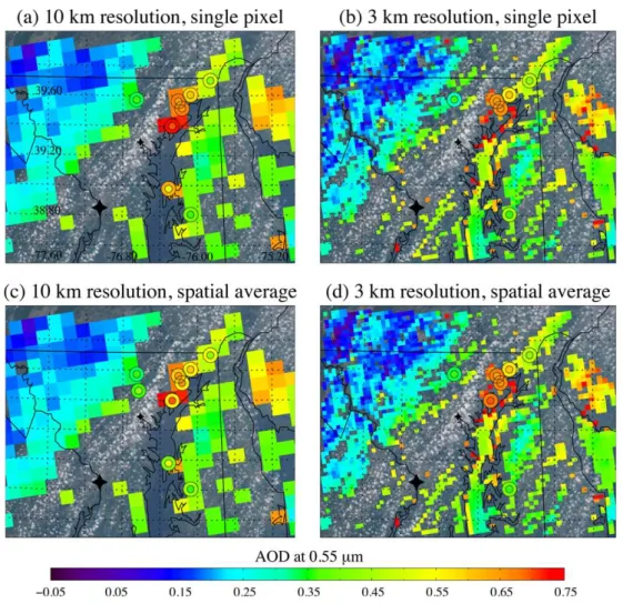
Fig. 1.AOD at 0.55 µm observed by MODIS-Aqua on 21 July 2011 at 18:30 UTC is plotted at the 10 km resolution (aandc) and 3 km resolution (bandd). MODIS/SP collocations are plotted in the circles. In(a–d), the inner circle is the SP temporally averaged AOD, which is an average of≥2 SP measurements within 30 min of MODIS overpass. In(a)and(b), the outside circle is the AOD of the MODIS pixel containing the SP site. In(c)and(d), the outer circle is the spatial average of a MODIS AOD in a 5×5 pixel box around the SP station. Only land pixels with a QA = 3 are used in the collocation. Washington D.C. is shown with the large black star and Baltimore, MD is shown with the small black star. The true color image, created from the MODIS red, green and blue bands, is shown in the background.
more detail and retrieves more area than the 10 km product. The 3 km product is also able to retrieve over bodies of wa-ter which are too narrow for 10 km retrievals, and has more pixels near the coastline that are unable to be retrieved by the 10 km product. The ability to retrieve closer to coastline is particularly valuable for air quality applications because many major cities, including some of the largest and most polluted, are located on coasts. This granule not only high-lights the value of a high resolution satellite product, but also shows that AOD can vary significantly over small distances. Plotted overtop of the MODIS AOD images in the circles are MODIS/SP collocations. In all of the panels (a–d), the inner circle shows the SP temporal mean, which is calcu-lated by averaging all SP 0.55 µm AOD measurements at a station within 30 min of the MODIS overpass time, with a minimum of 2 observations. In the top row (panels a and b), the outer circle shows the 0.55 µm AOD of the MODIS pixel
Fig. 2.AOD at 0.55 µm observed by MODIS-Terra on 1 July 2011 at 15:35 UTC is plotted at the 10 km resolution (aand c) and 3 km resolution (bandd). MODIS/SP collocations are plotted in the circles. In(a–d), the inner circle is the SP temporally averaged AOD, which is average of≥2 SP measurements within 30 min of MODIS overpass. In(a)and(b), the outside circle is the AOD of the MODIS pixel containing the SP site. In(c)and(d), the outer circle is the spatial average of a MODIS AOD in a 5×5 pixel box around the SP station. Only land pixels with a QA = 3 are used in the collocation. Washington D.C. is shown with the large black star and Baltimore, MD is shown with the small black star. The true color image, created from the MODIS red, green and blue bands, is shown in the background.
does increase the number of MODIS-SP collocations as com-pared to the single pixel technique, adding an extra collo-cation for each product. This granule shows that the single pixel collocation technique better characterizes AOD at the SP site, but limits the number of collocations and therefore the statistical robustness of the validation.
Figure 2 shows the 10 km and 3 km resolution MODIS AOD observed by MODIS-Terra on 1 July 2011 at 15:35 UTC, which has a markedly different aerosol distri-bution than that shown in Fig. 1. On this day, AOD is low (0.12 as measured by the SPs) and is homogeneous across the region. As in Fig. 1, the large-scale view of the two MODIS products agree, but there are nuanced differences. Some noisy pixels are present in the 3 km product, and are less apparent in the 10 km product. Both the 10 km and 3 km products have elevated AOD along the New Jersey and Delaware coastline, which are plausibly cloud contaminated
from subpixel clouds. The 10 km has fewer contaminated pixels, but they extend further from the coastline; the 3 km product has more contaminated pixels, but their spatial ex-tent is limited to right along the coastline. The 3 km product also shows a small amount of striping that results from dif-ferences in the MODIS instrument detectors. As in Fig. 1, the 3 km product has more coverage over the water areas in this scene. The MODIS/SP collocation circles are as they were in Fig. 1, with MODIS single pixel collocations shown in the outer circles of the top row, MODIS spatial average colloca-tions in the outer circles of the bottom row, and SP temporal averages in the inner circle of all panels.
0.55 µm AOD at the SP stations is 0.15, only 0.03 higher than the SP determined AOD. The MODIS 3 km spatially aver-aged collocations show an AOD enhancement of 0.1 to 0.3 over Baltimore City that is not observed by the SP measure-ments; 9 out of the 26 MODIS 3 km spatial averages shown in Fig. 2d have an above expected error. The largest differ-ence between the MODIS 3 km and SP measurements was observed at the sun photometer station in Essex, Maryland, 13 km east of downtown Baltimore, where the SP AOD is 0.11, and the AOD of the 3 km spatial average is 0.38. A similar AOD enhancement is seen over Washington D.C., al-though there are no SP measurements to confirm that this enhancement is a retrieval artifact. The single MODIS pixel collocations in the Fig. 2b do not capture this important re-trieval problem due to the coincidences of where the SP sta-tions happen to be located and if the exact pixel where the station is located is retrieved. This case study suggests that the spatial average collocation technique better character-izes the retrieval performance over the larger region, and the single pixel collocation technique may misrepresent product performance because it is much more sensitive to the siting of the SP stations.
The airborne HSRL measurements provide an opportu-nity to look at aerosol extinction and AOD spatial variabil-ity with a nominal 1 min resolution, which corresponds to a nearly 6 km horizontal resolution. Figure 3 shows an-other high aerosol loading day, observed by MODIS-Terra on 29 July 2011 at 16:00 UTC. HSRL 532 nm columnar AOD along the flight track between 15:30 and 16:30 UTC is shown in the thick line, plotted atop of the 3 km resolution 0.55 µm AOD. The sections of the flight track where the plane was flying lower than 7 km, flying above clouds, or was turn-ing are shown in grey. SP AOD interpolated to 0.55 µm is shown in the circles. The SP measurements are not tem-porally averaged; the nearest measurement to 16:00 UTC is used, provided the measurement was taken between 15:30 and 16:30 UTC.
The SP AOD measurements range from 0.33 to 0.58, with lower values towards the south and west, and higher val-ues towards the north and east. The HSRL AOD measure-ments have a wider range from 0.35 to 0.67. There is excel-lent agreement between HSRL and SP measurements at the AERONET stations, which indicates that the broader range of AOD values from HSRL is likely due to the HSRL instru-ment being able to measure a larger area than the sun pho-tometers and not due to inaccuracies in either measurement. The MODIS 3 km product generally captures the spatial pat-tern of AOD as observed by both the HSRL instrument and the sun photometers, although as in Fig. 2, the AOD is over-estimated in the urban areas and there are noisy retrievals. Outside of the urban areas, the MODIS image shows AOD near 0.45 for much of the southern and western portion of the granule, increasing to 0.65–0.75 in the northeastern por-tion of the granule that also has HSRL and SP measurements.
ï77.40 ï77.00 ï76.60 ï76.20 ï75.80
38.40 38.80 39.20 39.60
AOD
ï0.05 0.05 0.15 0.25 0.35 0.45 0.55 0.65 0.75
Fig. 3.A 3 km resolution AOD at 0.55 µm observed by MODIS-Terra on 29 July 2011 at 16:00 UTC is plotted in the background. HSRL 532 nm columnar AOD along the flight track between 15:30 and 16:30 UTC is shown in the thick line. SP AOD interpolated to 0.55 µm is shown in the circles. The SP measurements are not temporally averaged; the nearest measurement to 16:00 UTC is shown, provided the measurement was taken between 15:30 and 16:30 UTC. Washington D.C. is shown with the large black star and Baltimore, MD is shown with the small black star. The true color image, created from the MODIS red, green and blue bands, is shown in the background.
Overall, the three instruments show a similar aerosol situa-tion albeit with varying levels of detail.
(a) 10 km product
ï76.68 ï76.60 ï76.52 ï76.44 ï76.36 38.85
38.95 39.05 39.15
(b) 3 km product
AOD
ï0.05 0.05 0.15 0.25 0.35 0.45 0.55 0.65 0.75
Fig. 4.Close up view of the area enclosed in the white box in Fig. 3.(a)MODIS 10 km 0.55 µm AOD with 532 nm HSRL AOD plotted on top.(b)MODIS 3 km 0.55 µm AOD with 532 nm HSRL AOD plotted on top.
of the contamination and allows nearby uncontaminated pix-els to retrieve the correct AOD. In the 3 km product, the ef-fects of cloud or surface contamination are larger within a single pixel, but at the same time are also spatially limited.
As highlighted in Fig. 4, because the HSRL instrument makes several measurements within a single MODIS pixel, it provides an opportunity to assess AOD variability across the standard MODIS retrieval resolution. A measure of subpixel AOD variability is shown in Fig. 5. For each 10 km resolution MODIS pixel, the minimum HSRL measured AOD is sub-tracted from the maximum HSRL AOD, provided the mea-surements are within half an hour of the MODIS overpass. Data from all flights that have valid data within half an hour of a MODIS overpass are included, and only MODIS pix-els that contain more than 5 HSRL observations are ana-lyzed to ensure that two fully independent HSRL measure-ments are obtained within the MODIS pixel. In all, 482 MODIS pixels are available for analysis for subpixel AOD variations. Within a single MODIS 10 km pixel, the maxi-mum HSRL measured AOD change is 0.25, increasing from 0.36 to 0.61 AOD. The mean 0.55 µm AOD variation within a 10 km pixel is 0.037 while the median variation within a 10 km pixel is 0.023. Fewer than 25 % of pixels contained less than 0.01 AOD variation. The 10 km retrieval assumes uniformity of the AOD across the retrieval box, and that is simply not the case. The assumption is likely to hold bet-ter across the 3 km retrieval box; however, the nominal res-olution of the HSRL instrument for this study is larger than the 3 km retrieval box. For this case, decreasing the HSRL nominal horizontal resolution for AOD from 6 km to 1 km increased the noise to an unacceptably high level such that
0.00 0.05 0.10 0.15 0.20
HSRL AOD Range 0.00
0.05 0.10 0.15 0.20 0.25
Normalized Frequency
10 km
Fig. 5. The maximum difference between HSRL 0.55 µm AOD measurements observed within a MODIS 10 km pixel, normalized by the total number of analyzed grid boxes. Only MODIS pixels that contain 6 or more HSRL measurements are included.
the AOD variation within the MODIS 3 km pixels could not be quantified.
(a) Single pixel ï 10 km
0.0 0.2 0.4 0.6 0.8 1.0 AERONET 0.55 µm AOD 0.0 0.2 0.4 0.6 0.8 1.0 MODIS 0.55 µ m AOD
(b) Single pixel ï 3 km
0.0 0.2 0.4 0.6 0.8 1.0 AERONET 0.55 µm AOD 0.0 0.2 0.4 0.6 0.8 1.0 MODIS 0.55 µ m AOD 1 2 3 4 5 Frequency
(c) Single pixel
0.0 0.1 0.2 0.3 0.4 0.5 0.6 AERONET 0.55 µm AOD
ï0.2 ï0.1 0.0 0.1 0.2 MODIS ï AERONET 0.55 µ m AOD
10 km product 3 km product
(d) Spatial average ï 10 km
0.0 0.2 0.4 0.6 0.8 1.0 AERONET 0.55 µm AOD 0.0 0.2 0.4 0.6 0.8 1.0 MODIS 0.55 µ m AOD
(e) Spatial average ï 3 km
0.0 0.2 0.4 0.6 0.8 1.0 AERONET 0.55 µm AOD 0.0 0.2 0.4 0.6 0.8 1.0 MODIS 0.55 µ m AOD 1 2 3 4 5 Frequency
(f) Spatial average
0.0 0.1 0.2 0.3 0.4 0.5 0.6 AERONET 0.55 µm AOD
ï0.2 ï0.1 0.0 0.1 0.2 MODIS ï AERONET 0.55 µ m AOD
10 km product 3 km product
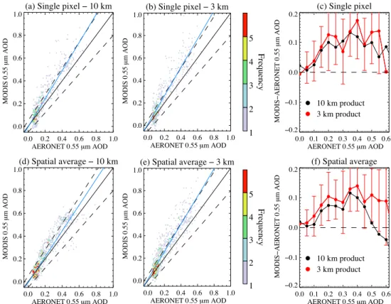
Fig. 6. (a)Density scatter plot of MODIS/SP collocations for 10 km AOD at 0.55 µm, using the single pixel collocation technique. Expected error over land (±0.05±0.15 AOD) is shown in the dashed lines, the best fit line is shown by the solid blue line, and the one-to-one line is shown in the solid black line.(b)Same as in(a), except for the 3 km product.(c)Average difference between MODIS single pixel collocations and SP 0.55 µm AOD, as a function of SP 0.55 µm AOD. A standard deviation of±1 is shown for the 3 km product.(d–f)As in(a–c), except the MODIS 5×5 pixel spatial average collocation is used.
small changes in AOD over an urban/suburban region. How-ever, retrieving with a higher resolution reduces the statistical robustness of the aerosol product, resulting in more noise and inaccurate retrievals over urban areas.
4.2 MODIS 3 km validation
The case studies highlight the strengths and weaknesses of the 3 km product; however, the sun photometer data from the entire campaign provides the most comprehensive dataset to characterize its performance. The SP data also allows a crit-ical look at how the different collocation techniques demon-strated in Figs. 1 and 2 lead to different conclusions on the validity on the MODIS AOD data in this region for both the 10 and 3 km resolutions.
In Fig. 6a, all 10 km MODIS/SP 0.55 µm AOD colloca-tions are shown in a density scatter plot, using the MODIS single pixel collocation technique employed in Figs. 1a and 2a, and the same is shown in Fig. 6b for the 3 km product. In Fig. 6c, these single pixel MODIS/SP collocations are binned by the SP AOD, and the mean MODIS-SP difference for the bin is plotted for both the 10 and 3 km products. This process is repeated in Fig. 6d–f except that the 5×5 pixel MODIS spatial collocation technique is employed in the MODIS/SP
collocations. The collocation statistics for both techniques for both products is shown in Table 1.
For both MODIS/SP collocation techniques, the bulk of the 3 km MODIS retrievals are within the±0.05±0.15 AOD expected error (63.6 % for the single pixel technique and 68 % for the spatial average technique). The satellite retrieval is highly correlated with the ground-based measurements, although with a small negative offset (0.011 for the single pixel technique and 0.013 for the spatial average technique) and a significant slope (1.26 for single pixel, 1.22 for spatial average). Accordingly, the MODIS 3 km AOD agrees well with SP AOD at low aerosol loadings, but is generally biased high at higher AOD. The primary difference between the two collocation techniques is that the spatial average has nearly twice as many collocations (817 as opposed to 451, for the 3 km product); therefore, the spatial averaging technique may be more representative of the region at large.
Table 1.Statistics from the 4 different MODIS/SP collocations shown in Fig. 6a,b and d–e.N= number of valid collocations,R= correlation coefficient, Slope = slope of regression line (shown in blue in Fig. 6), Offset =yintercept of the regression line, bias = MODIS average AOD minus SP average AOD, RMSE = root mean square error of collocations. EE for all cases is±0.05±0.15 AOD.
Product Averaging % above % within % below
resolution method N R Slope Offset Bias RMSE EE EE EE
10 km single pixel 499 0.925 1.235 0.004 0.049 0.093 26.7 69.3 4.0
10 km spatial average 848 0.935 1.134 0.008 0.039 0.075 21.5 75.9 2.6
3 km single pixel 451 0.914 1.263 0.011 0.062 0.109 33.7 63.6 2.7
3 km spatial average 817 0.928 1.228 0.013 0.057 0.096 30.7 68.0 1.3
(a) 10 km resolution
0.0 0.2 0.4 0.6 0.8 1.0 HSRL 532 nm AOD 0.0
0.2 0.4 0.6 0.8 1.0
MODIS 0.55
µ
m AOD
% within EE = 53.56 % above EE = 46.00 % below EE = 0.43 N = 1613; R = 0.88 Y= 1.01x+ 0.07
(b) 3 km resolution
0.0 0.2 0.4 0.6 0.8 1.0 HSRL 532 nm AOD 0.0
0.2 0.4 0.6 0.8 1.0
MODIS 0.55
µ
m AOD
% within EE = 56.05 % above EE = 42.04 % below EE = 1.92 N = 1199; R = 0.82 Y= 0.94x+ 0.07
1 2 3 4 5 6 7 8 9 10
Frequency
Fig. 7.Density scatter plot of MODIS/HSRL collocations for AOD at 0.55 µm for MODIS and 532 nm for HSRL for the 10 km MODIS product(a)and the 3 km MODIS product(b). The MODIS AOD is sampled along the HSRL flight path; no spatial or temporal averaging is performed. Expected error over land (±0.05±0.15 AOD) is shown in the dashed lines, the best fit line is shown by the solid blue line, and the one-to-one line is shown in the solid black line.
the different products. The 3 km product single pixel aver-ages shown in Fig. 6c show that the average AOD of the 3 km product is frequently, but not always, higher than the 10 km product.
The retrieved AOD from the HSRL airborne instrument provides a different perspective on validation of the 3 km product. Because the plane is moving quickly in space, no spatial or temporal averaging is used to make the MODIS/HSRL collocations. The MODIS data are sampled along the HSRL flight track, provided that the HSRL ob-servation is made within the geographic region mapped in Figs. 1 and 2, and is within 30 min of the MODIS overpass. Shortening the time requirement to either 15 or 5 min does not significantly affect the collocation statistics, but provides far fewer collocations. The HSRL and MODIS AOD are not interpolated to the same wavelength, which is expected to introduce between 2–4 % error (Kittaka et al., 2011). It is expected that the AOD retrieved by the HSRL instrument would be lower than the AOD retrieved by MODIS by at least 0.01 to 0.02 because the HSRL instrument does not measure the entire column, and therefore neglects the contribution of above the HSRL profile (i.e. above 7 km) to total columnar AOD.
Figure 7 shows that the both products agree with HSRL, but with significant high bias (0.093 for 10 km, 0.086 for 3 km). The increased bias of the 10 km product could be due to the pixel contamination effect shown in Fig. 4 – al-though the 3 km product contains more contaminated pixels, the spatial extent of those pixels is limited, allowing more correct pixels as well. The 10 km MODIS/HSRL comparison also shows the necessity of a higher resolution retrieval; the stripes in the HSRL/MODIS comparison show the change in HSRL AOD within a single pixel; the pattern that is quanti-fied in Fig. 5.
ï77.40 ï77.00 ï76.60 ï76.20 ï75.80
38.40 38.80 39.20 39.60
Percent within expected error
0 10 20 30 40 50 60 70 80 90 100
Correlation coefficient (R)
0.75 0.80 0.85 0.90 0.95 1.00
Fig. 8. (a)Percent of 3 km spatially averaged MODIS/SP collocations of 0.55 µm AOD within expected error (±0.05±0.15 AOD) at each SP station.(b)Correlation coefficient between 3 km spatially averaged MODIS 0.55 µm AOD and SP temporally averaged 0.55 µm measure-ments at each station. Land identified as urban/built up by the MODIS land cover product (MCD12Q1) is plotted in grey in both panels.
measurements. The single pixel and spatial average MODIS collocation techniques show quantitative but not qualitative differences.
4.3 Sources of uncertainty
Figures 2 and 3 show an overestimation of AOD in urban areas. In order to study this further, we separate the 3 km MODIS/SP spatially averaged collocations by SP station, and compute agreement statistics for each station. We choose the spatial averaging collocation technique because it pro-vides more collocations. The percent of comparisons within expected error for each station is shown in Fig. 8a, and the correlation coefficient (R) between MODIS and SP 0.55 µm AOD is shown in Fig. 8b. In each panel, land classified as “ur-ban” by the MODIS Land Cover type product (MCD12Q1) is plotted in grey.
Figure 8a shows remarkable variability in the percent of collocations within EE for each SP station, ranging between 16 % to 95 %. The stations with the smallest percent within EE are clustered around the Baltimore urban center, and the more urbanized I-95 corridor between Washington D.C. and Baltimore. However, the stations with small percentages of collocations within EE still have correlation coefficients above 0.85, suggesting that the error is a systematic bias that could be accounted for in future retrievals, and not a random error.
We wish to quantify the urban overestimation of the 3 km product using the dense spatial distribution of the sun pho-tometer sites in the DRAGON network. Using the same 15 km averaging box as the MODIS spatial collocation, the percent of pixels within the averaging box identified as ur-ban by the MCD12Q1 product is calculated. In Fig. 9, this quantity is plotted against the percent of collocations above EE for each SP site. The percent of urban land within the MODIS averaging box is well correlated with the percent
0 20 40 60 80 100
Urban landcover percentage 0
20 40 60 80 100
Percent of colocations above EE
Y = 0.93x + 12.83 R = 0.91
Fig. 9.Percent of 3 km spatially averaged MODIS/SP 0.55 µm AOD collocations above expected error (+0.05 + 0.15 AOD) at each SP station, plotted against the percentage of pixels within the 15 km by 15 km collocation box identified as urban by the MODIS land cover product.
Fig. 10. (a)3 km AOD at 2.1 µm observed by MODIS-Aqua on 21 July 2011 at 18:30 UTC.(b)3 km AOD at 2.1 µm observed by MODIS-Terra on 1 July 2011 at 15:35 UTC. Only land pixels with a QA = 3 are shown. Washington D.C. is shown with the large black star and Baltimore is shown with the small black star. The true color image, created from the MODIS red, green and blue bands, is shown in the background.
the retrieval box after pixel selection, causing the surface reflectance in the visible wavelengths to be underestimated, leading to an overestimation in AOD.
Ideally, the noisy pixels could be flagged as poor quality, and therefore treated with some degree of caution. One of the products produced operationally is the AOD at 2.1 µm. This is not a validated product, but is used as a diagnos-tic to the retrieval. It may hold information that can identify poorer quality 3 km retrievals. In Fig. 10a, the 2.1 µm AOD on 21 July 2011 at 18:30 from the 3 km product is plotted, the same granule as that shown in Fig. 1b, and in Fig. 10b; the 2.1 µm AOD on 1 July 2011 at 15:35 UTC from the 3 km product is plotted, the same granule as that shown in Fig. 2b. The scene-wide 2.1 µm AOD is 0.046 in the left panel, and is 0.065 in the right panel. Both granules contain pixels with a 2.1 µm AOD over 0.2, more than 3 to 5 times higher than the scene-wide average. The error is not due to the wrong aerosol model being picked; in both scenes, all of the pix-els were assigned the fine mode dominated urban aerosol model (Levy et al., 2007a). It appears that the same pix-els that have anomalously high 2.1 µm AOD retrievals also tend to have inaccurate 0.55 µm AOD retrievals. For exam-ple, the pixels with high (>0.55) AOD in Fig. 1b that agree with SP observations have retrieved 2.1 µm AOD values that do not stand out from the background. However, the pixels with high AOD in Fig. 2b that do not agree with SP observa-tions have retrieved 2.1 µm AOD values significantly higher than the background. Although the 2.1 µm AOD retrieval is an unvalidated product, it may serve a purpose as a consis-tency check in this fine mode dominated, urban environment. This consistency check is likely to be inapplicable in dusty or other coarse mode dominated regimes.
Using anomalous 2.1 µm AOD pixels as a proxy for poor quality 0.55 µm pixels, and therefore throwing them out, re-sults in a reduction of the both the negative bias at low AOD and the positive bias at high AOD. If the 3 km product is filtered such that pixels with a 2.1 µm AOD over 0.2 are ex-cluded, and MODIS/SP are collocated using the spatial av-eraging technique, the percent within EE rises from 68 % to 78 %, while the number of collocations falls from 817 to 727, and theR rises from 0.92 to 0.95. However, this screening is not globally applicable, and is not recommended for use without closer examination.
It appears that a primary source of error in the 3 km MODIS aerosol product is the incorrect estimation of surface reflectance over urban regions. This error is not as apparent in the 10 km product because brighter urban surfaces are pref-erentially discarded during the pixel selection process. How-ever, because the 3 km product has a smaller footprint, it is likely that not all urban pixels are discarded, and the surface reflectance is underestimated, leading to an overestimation in AOD. The 2.1 µm AOD shows some potential as an imperfect filter for these poor quality pixels.
5 Summary and conclusions
produced at a 3 km resolution will be available in MODIS Collection 6.
This new product was evaluated against ground and air-borne data over the Baltimore–Washington D.C., USA cor-ridor over the summer of 2011 to understand the poten-tial added information from the higher resolution retrieval and the statistical reliability of the product. The 10 km and 3 km granules generally resolve similar large scale patterns in aerosol distribution but differ in the details. The smaller foot-print of the 3 km product retrieves closer to clouds and over small bodies of water, but also makes the product more sus-ceptible to cloud contamination and other sources of noise. Subpixel comparisons against HSRL show that AOD can vary significantly within a 10 km pixel, and a 3 km resolution is a more appropriate scale for studying aerosol distributions in urban and suburban settings.
The dense network of sun photometers deployed during the DISCOVER-AQ campaign provided an unprecedented opportunity to validate aerosol products at a high spatial scale. Given the new resolution of both the satellite data and the ground validation network, the MODIS spatial-temporal collocation techniques for validation were revisited. It was found that using a spatial average of MODIS pixels around a sun photometer station, or using only the pixel where the SP station is located resulted in a quantitative, but not qualita-tive, difference. We conclude with good confidence that the MODIS 3 km validates in this region, but is biased high at AOD values greater than 0.1.
There is evidence that a significant source of the bias ob-served in the 3 km product results from improper characteri-zation of urban surfaces. The method for attributing the sur-face contributions to TOA measured reflectances has been documented to underestimate the surface reflectances in ur-ban areas (Castanho et al., 2008; Oo et al., 2010), which in turn overestimates AOD. Indeed, we found a strong cor-relation between the amount of urban surface near a sun photometer station, and the percent of collocations that are above the expected error. While case studies show that the 10 km product also has one or two pixels that are affected, the smaller pixel size of the 3 km product causes it to be more susceptible to contamination.
The poor performance of the 3 km product over urban sur-faces is clearly a limitation in terms of air quality applica-tions. How to best address this problem in an operational en-vironment remains an open question. However, despite this limitation, the 3 km aerosol product has new capabilities for studying aerosol on local scales, including resolving small scale AOD gradients and point sources, retrieving aerosol in patchy cloud fields, and retrieving closer to coastlines. We expect that the added information of the 3 km resolution product will complement the existing MODIS 10 km reso-lution aerosol product and products from other passive and active sensors to provide a more complete view of global aerosol properties from space.
Acknowledgements. The authors thank Bill Ridgway and the MODAPS team for facilitating iterative testing needs. We also thank the University of Wisconsin PEATE team for the production of the Terra L1B data used in previous iterations of this study. We recognize the entire AERONET team for their efforts to deploy and maintain 44 functioning AERONET stations. HSRL operations were funded by the NASA DISCOVER-AQ program. The authors also thank the NASA Langley King Air flight crew for their outstanding work supporting these flights.
Edited by: M. King
References
Bellouin, N., Boucher, O., Haywood, J., and Reddy, M. S.: Global estimate of aerosol direct radiative forcing from satellite mea-surements, Nature, 438, 1138–1141, 2005.
Castanho, A. D., Martins, J. V., and Artaxo, P.: MODIS Aerosol Optical Depth Retrievals with high spatial resolution over an Ur-ban Area using the Critical Reflectance, J. Geophys. Res., 113, D02201, doi:10.1029/2007JD008751, 2008.
Chu, D. A.: Global monitoring of air pollution over land from the Earth Observing System-Terra Moderate Resolution Imag-ing Spectroradiometer (MODIS), J. Geophys. Res., 108, 4661, doi:10.1029/2002JD003179, 2003.
Eck, T. F., Holben, B. N., Reid, J. S., Dubovik, O., Smirnov, A., O’Neill, N. T., Slutsker, I., and Kinne, S.: Wavelength depen-dence of the optical depth of biomass burning, urban and desert dust aerosols, J. Geophys. Res., 104, 31333–31350, 1999. Engel-Cox, J. A., Holloman, C. H., Coutant, B. W., and Hoff, R. M.:
Qualitative and quantitative evaluation of MODIS satellite sensor data for regional and urban scale air quality, Atmos. Environ., 38, 2495–2509, 2004.
Friedl, M. A., Sulla-Menashe, D., Tan, B., Schneider, A., Ra-mankutty, N., Sibley, A., and Huang, X.: MODIS Collection 5 global land cover: Algorithm refinements and characterization of new datasets, Remote Sens. Environ., 114, 168–182, 2010. Hair, J. W., Hostetler, C. A., Cook, A. L., Harper, D. B., Ferrare, R.
A., Mack, T. L., Welch, W., Izquierdo, L. R., and Hovis, F. E.: Airborne high spectral resolution LIDAR for profiling aerosol optical properties, Appl. Optics, 47, 6734–6752, 2008.
Hutchison, K. D.: Applications of MODIS satellite data and prod-ucts for monitoring air quality in the state of Texas, Atmos. Env-iron., 37, 2403–2412, 2003.
Hutchison, K. D., Smith, S., and Faruqui, S.: The use of MODIS data and aerosol products for air quality prediction, Atmos. Env-iron., 38, 5057–5070, 2004.
Holben, B. N., Eck, T. F., Slutsker, I., Tanre, D., Buis, J. P., Set-zer, A., Vermote, E., Reagan, J. A., Kaufman, Y. J., Nakajima, T., Lavenu, F., Janowiak, I., and Smirnov, A.: AERONET – A federated instrument network and data archive for aerosol char-acterization, Remote Sens. Environ., 66, 1–16, 1998.
Hsu, N. C., Tsay, S. C., King, M. D., and Herman, J. R.: Aerosol Properties Over Bright-Reflecting Source Regions, Ieee T. Geosci. Remote, 42, 557–569, 2004.
Ichoku, C., Chu, D. A., Mattoo, S., Kaufman, Y. J., Remer, L. A., Tanr´e, D., Slutsker, I., and Holben, B. N.: A spatio-temporal approach for global validation and analysis of MODIS aerosol products, Geophys. Res. Lett., 29, MOD1.1–MOD1.4, doi:10.1029/2001GL013206, 2002.
IPCC1: AR4 WG, Climate Change 2007: The Physical Science Ba-sis, Contribution of Working Group I to the Fourth Assessment Report of the Intergovernmental Panel on Climate Change, edited by: Solomon, S., Qin, D., Manning, M., Chen, Z., Marquis, M., Averyt, K. B., Tignor, M., and Miller, H. L., Cambridge Univer-sity Press, ISBN 978-0-521-88009-1, 2007.
Kaufman, Y. J., Tanr´e, D., Remer, L., Vermote, E., Chu, A., and Hol-ben, B.: Operational remote sensing of tropospheric aerosol over land from EOS moderate resolution imaging spectroradiometer, J. Geophys. Res., 102, 17051–17067, 1997a.
Kaufman, Y. J., Wald, A., Remer, L., Gao, B., Li, R., and Flynn, L.: The MODIS 2.1 µm channel – Correlation with visible re-flectance for use in remote sensing of aerosol, IEEE T. Geosci. Remote, 35, 1286–1298, 1997b.
Kaufman, Y. J., Tanr´e, D., and Boucher, O.: A satellite view of aerosols in the climate system, Nature, 419, 215–223, 2002. Kittaka, C., Winker, D. M., Vaughan, M. A., Omar, A., and Remer,
L. A.: Intercomparison of column aerosol optical depths from CALIPSO and MODIS-Aqua, Atmos. Meas. Tech., 4, 131–141, doi:10.5194/amt-4-131-2011, 2011.
Levy, R. C., Remer, L. A., and Dubovik, O.: Global aerosol opti-cal properties and application to Moderate Resolution Imaging Spectroradiometer aerosol retrieval over land, J. Geophys. Res.-Atmos., 112, D13210, doi:10.1029/2006JD007815, 2007a. Levy, R. C., Remer, L. A., Mattoo, S., Vermote, E. F., and
Kauf-man, Y. J.: Second-generation operational algorithm: Retrieval of aerosol properties over land from inversion of Moderate Resolu-tion Imaging Spectroradiometer spectral reflectance, J. Geophys. Res.-Atmos., 112, D13211, doi:10.1029/2006JD007811, 2007b. Levy, R. C., Remer, L. A., Kleidman, R. G., Mattoo, S., Ichoku, C., Kahn, R., and Eck, T. F.: Global evaluation of the Collection 5 MODIS dark-target aerosol products over land, Atmos. Chem. Phys., 10, 10399–10420, doi:10.5194/acp-10-10399-2010, 2010. Levy, R. C., Mattoo, S., Munchak, L. A., Remer, L. A., Sayer, A. M., and Hsu, N. C.: The Collection 6 MODIS aerosol products over land and ocean, Atmos. Meas. Tech. Discuss., 6, 159–259, doi:10.5194/amtd-6-159-2013, 2013.
Li, C. C., Lau, A. K. H., Mao, J. T., and Chu, D. A.: Retrieval, val-idation, and application of the 1-km aerosol optical depth from MODIS measurements over Hong Kong, IEEE T. Geosci. Re-mote, 43, 2650–2658, 2005.
Li, R.-R., Kaufman, Y. J., Gao, B.-C., and Davis, C. O.: Remote sensing of suspended sediments and shallow coastal waters, IEEE T. Geosci. Remote, 41, 559–566, 2003.
Li, R., Remer, L., Kaufman, Y., Mattoo, S., Gao, B., and Vermote, E.: Snow and ice mask for the MODIS aerosol products, IEEE Geosci. Remote Sens. Lett., 2, 306–310, 2005.
Li, Y., Xue, Y., He, X., and Guang, J.: High resolution aerosol re-mote sensing retrieval over urban areas by synergetic use of HJ-1 CCD and MODIS data, Atmos. Environ., 46, 173–180, 2012.
Loveland, T. R. and Belward, A. S.: The IGBP-DIS global 1km land cover data set, DISCover: first results, Int. J. Remote Sens., 18, 3289–3295, 1997.
Lyapustin, A., Wang, Y., Laszlo, I., Kahn, R., Korkin, S., Remer, L., Levy, R., and Reid, J. S.: Multiangle implementation of atmo-spheric correction (MAIAC): 2. Aerosol algorithm, J. Geophys. Res.-Atmos., 116, D03211, doi:10.1029/2010JD014986, 2011. Martins, J. V., Tanr´e, D., Remer, L. A., Kaufman, Y. J., Mattoo,
S., and Levy, R.: MODIS Cloud Screening for Remote Sens-ing of Aerosol over Oceans usSens-ing Spatial Variability, Geophys. Res. Lett., 29, MOD4.1–MOD4.4, doi:10.1029/2001GL013252, 2002.
Oo, M. M., Jerg, M., Hernandez, E., Picon, A., Gross, B. M., Moshary, F., and Ahmed, S. A.: Improved MODIS aerosol re-trieval using modified VIS/SWIR surface albedo ratio over urban scenes, IEEE T. Geosci. Remote, 48, 983–1000, 2010.
Quaas, J., Boucher, O., Bellouin, N., and Kinne, S.: Satellite-based estimate of the direct and indirect aerosol climate forcing, J. Geo-phys. Res., 113, D05204, doi:10.1029/2007JD008962, 2008. Remer, L. A., Kaufman, Y. J., Tanre, D., Mattoo, S., Chu, D. A.,
Martins, J. V., Li, R. R., Ichoku, C., Levy, R. C., Kleidman, R. G., Eck, T. F., Vermote, E., and Holben, B. N.: The MODIS aerosol algorithm, products, and validation, J. Atmos. Sci., 62, 947–973, 2005.
Remer, L. A., Kleidman, R. G., Levy, R. C., Kaufman, Y. J., Tanre, D., Mattoo, S., Martins, J. V., Ichoku, C., Koren, I., Yu, H., and Holben, B. N.: Global aerosol climatology from the MODIS satellite sensors, J. Geophys. Res. Atmos., 113, D14S07, doi:10.1029/2007JD009661, 2008.
Remer, L. A., Mattoo, S., Levy, R. C., and Munchak, L.: MODIS 3 km aerosol product: algorithm and global perspective, Atmos. Meas. Tech. Discuss., 6, 69–112, doi:10.5194/amtd-6-69-2013, 2013.
Schmid, B., Michalsky, J., Halthore, R., Beauharnois, M., Harrison, L., Livingston, J., Russell, P., Holben, B., Eck, T., and Smirnov, A.: Comparison of aerosol optical depth from four solar radiome-ters during the fall 1997 ARM intensive observation period, Geo-phys. Res. Lett., 26, 2725–2728, 1999.
Smirnov, A., Holben, B. N., Eck, T. F., Dubovik, O., and Slutsker, I.: Cloud screening and quality control algorithms for the AERONET database, Remote Sens. Environ, 73, 337–349, 2000. Tanr´e, D., Kaufman, Y. J., Herman, M., and Mattoo, S.: Remote sensing of aerosol properties over oceans using the MODIS/EOS spectral radiances, J. Geophys. Res.-Atmos., 102, 16971–16988, 1997.
van Donkelaar, A., Martin, R. V., and Park, R. J.: Estimat-ing ground-level PM2.5 with aerosol optical depth determined from satellite remote sensing, J. Geophys. Res., 111, D21201, doi:10.1029/2005JD006996, 2006.