Study on Meshfree Hermite Radial Point Interpolation Method for
Flexural Wave Propagation Modeling and Damage Quantification
1 INTRODUCTION
Wave propagation can be used to identify the damage of small defects. The identification methods are based on high frequency excitation, wave interaction with the damage and scattering. A variety of numerical techniques were proposed to model wave propagation in time, frequency or time-frequency domains. The frequent scheme is finite element method (FEM) that its capability in this field was illustrated in references (Moser et al. 1999, Chakraborty et al. 2002). The high frequency loads are accompanying with shorter wavelength; therefore a large number of meshes and degrees of
Hosein Ghaffarzadeh a Majid Barghian a Ali Mansouri a,* Morteza.H Sadeghi b
a Department of Structural Engineering,
Faculty of Civil Engineering,University of Tabriz, Tabriz, East Azerbaijan Prov-ince, Iran
b Vibration and Modal Analysis
Labora-tory, Faculty of Mechanical Engineering, University of Tabriz, Tabriz, East Azer-baijan Province, Iran
*PhD student, [email protected]
http://dx.doi.org/10.1590/1679-78252890
Received 27.02.2016 In revised form 21.07.2016 Accepted 25.07.2016 Available online 03.08.2016
Abstract
This paper investigates the numerical modeling of the flexural wave propagation in Euler-Bernoulli beams using the Hermite-type radial point interpolation method (HRPIM) under the damage quantifica-tion approach. HRPIM employs radial basis funcquantifica-tions (RBFs) and their derivatives for shape function construction as a meshfree technique. The performance of Multiquadric(MQ) RBF to the assessment of the reflection ratio was evaluated. HRPIM signals were compared with the theoretical and finite element responses. Results represent that MQ is a suitable RBF for HRPIM and wave propagation. However, the range of the proper shape parameters is notable. The number of field nodes is the main parameter for accu-rate wave propagation modeling using HRPIM. The size of support domain should be less thanan upper bound in order to prevent high error. With regard to the number of quadrature points, providing the minimum numbers of points are adequate for the stable solu-tion, but the existence of more points in damage region does not leads to necessarily the accurate responses. It is concluded that the pure HRPIM, without any polynomial terms, is acceptable but considering a few terms will improve the accuracy; even though more terms make the problem unstable and inaccurate.
Keywords
freedom are needed for the exact consideration of the wave energy. This limitation leads to the high cost computation which makesit necessary todevelop the alternative techniques. Modified FEM (Keramat and Ahmadi 2012), boundary element method (Zhao and Rose 2003), mass-spring lattice model (MSLM) (Yim and Sohn 2000) and several spectral FEM (Mitra and Gopalakrishnan 2005, Kudela et al. 2007) have been reported as novel algorithms for wave propagation and damage iden-tification. However mesh-based methods are not well suited to treat problems with strong inhomo-geneity, mesh distortion and discontinuities that do not align with element edges especially for dy-namic problems such as crack propagation (Chen et al. 2006, Nguyen et al. 2008). To overcome these drawbacks different meshfree schemes were introduced (Li and Liu 2007, Liu 2010, Li and Mulay 2013). Wen (2010) utilized the meshfree local Petrov–Galerkin (MLPG) method to solve wave propagation problem in three-dimensional poroelastic solids. Gao et al. (2007) proposed a new MLPG method to analyze stress-wave propagation in anisotropic and cracked media. Das and Kun-du (2009) simulated the ultrasonic wave field models for layered half-spaces with and without an internal crack using the meshfree semi-analytical distributed point source method. Zhang and Batra (2004) applied a modified smoothed particle hydrodynamics to study the 1D wave propagation and 2D transient heat conduction problems.
Among the various meshfree techniques, radial basis functions (RBFs) or, more generally, con-ditionally positive definite kernels have been achieved significant attention in approximation and the solution of partial differential equations (PDEs). RBFs are powerful tools to interpolate the multivariate scattered data. They are insensitive to spatial dimension, differentiable, computational-ly simple and stable in the interpolation (Buhmann 2003, Liew and Chen 2004, Wendland 2010). Hardy (1971) used multi-quadric (MQ) RBF to solve the approximation of a topographic surface. Franke (1982) explored MQ and some other scattered data interpolation methods to evaluation the timing, storage, accuracy and the ease of implementation. Lazzaro et al. (2002) proposed an efficient method for the multivariate interpolation of very large scattered data sets using RBF and Shepard’s method. Kansa (1990a,b) was the pioneer who used MQ for partial derivative estimates and solving of elliptic, parabolic, and hyperbolic PDEs. Kansa’s method searches an approximate solution in the function space using collocation technique by a set of RBFs. His method was extended to solve var-ious PDEs which can be referred in (Hon and Wu 2000, Fedoseyev et al. 2002, Tiago and Leitão 2006, Dehghan and Shokri 2009).
The Primary disadvantage of the traditional RBF approach is that the coefficient matrices ob-tained from discretization scheme are fully populated, which limit its application in large scale prac-tical problems (Wang and Liu 2000). One effective approach is the combination of radial and poly-nomial basis functions which was introduced by Wang and Liu (2002) as radial point interpolation method (RPIM). Point interpolation method (Liu and Gu 2001) satisfies Kronocker delta function property of shape functions and makes the implementation of essential boundary conditions easier but the matrix may be singular.Applying mentioned combination can guarantee the stability of shape functions and the improvement of singularity for arbitrarily and irregular node distribution (Liu 2010).
Gaussi-an interpolation in data fitting. KGaussi-ansa (1990a) proposed a scheme that allowed the shape parameter of MQ to vary with basis functions. Wang and Liu (2002) proposed optimal shape parameters for MQ and reciprocal MQ in 2D solid mechanics. Fornberg and Wright (2004) used a technique called Contour-Padé algorithm for stable computation of RBF approximation methods. The algorithm avoids working directly with the associated ill-conditioned linear systems for all values of the shape parameters. Bozkurt et al. (2013) discussed the effects of shape parameters on the RPIM accuracy in 2D geometrically nonlinear problems. Kanber et al. (2013) studied RPIM algorithm for the solu-tion of 2D elastoplastic problems using the multiquadric RBF. The convergence rates after yielding were investigated for perfectly plastic and hardening cases with various shape parameters. Both regular and irregular node distributions were used by considering the standard Gauss integration and nodal integration schemes.
The RPIM within the framework of weak form applied in various engineering problems: solid mechanics (Liew and Chen 2004, Liu et al. 2005, Liu et al. 2006), plate structures (Liew and Chen 2004), geometrical nonlinearity (Bozkurt et al. 2013), composite materials (Liu et al. 2008) and consolidation process (Wang et al. 2002). Ghaffarzadeh and mansouri (2013) studied the longitudi-nal wave propagation based on RPIM in rods. The capability of RPIM and the effect of MQ shape parameters were explored for detection of additional mass which is located in the length of the rod.
In some problems, derivatives of field functions should be considered as independent variables other than the function values. In this field, Wu (1992) introduced the Hermite RBF approach based on Hermite-Birkhoff interpolation for scattered multidimensional data. In solid mechanics, Liu et al. (2006) proposed Hermite radial point interpolation method (HRPIM) to approximate the deflection to solve the Kirchhoff plate problem using Galerkin weak form method. In their method, static analysis of different geometric shapes and boundary conditions verified the efficiency, accura-cy and robustness of the method. Cui et al. (2009) developed a smoothed HRPIM using gradient smoothing operation for thin plate analysis. The approximation of deflection and rotation variables made the proposed method very effective in enforcing the essential boundary conditions even for extremely irregular background cells.
This study is conducted to illustrate the performance of Hermite RPIM weak form for the mod-eling of elastic wave propagation and damage quantification. The model is Euler-Bernoulli beam which has the predefined step damage as a crack in the specific position. Damage quantification algorithm is based on the analytical solution of governed differential equation that yields the rela-tion between the reflecrela-tion ratio and depth of damage. The dispersive behavior of flexural waves is considered in solution. The reflection ratios are calculated from captured signals using Hilbert trans-form to achieve the energy envelope of signals. The field nodes density, the size of support domain, the values of shape parameters in MQ, the number of polynomials and integration points are the most important parameters which are investigates in this study.
2 PROBLEM FORMULATIONS
2.1 Hermite Radial Point Interpolation (HRPIM)
used to develop the radial point interpolation method (RPIM). Adding polynomial terms up to the linear order can ensure to pass the standard patch tests and for considering derivatives of field func-tions as independent variables, RPIM augments with derivatives of RBF. Therefore, the function
( )
u x is approximated by a linear combination of RBFs, its derivatives and polynomials as following for 1D beam model which has two degrees of freedom at each node along x-axis:
T T T
,
=1 =1 =1
T
T T T
,
( ) ( ) ( ) ( ) ( ) ( ) ( )
[ ( ) ( ) ( )]
n n m
h x
i i i,x i j j
i i j
x
u R a R a P b x x
x
x x x x R x a R x a P x b
R x R x P x a a b
(1)where Ri( )x and
R
i,x( )
x
are RBF and its derivative, respectively andP
j( )
x
is the polynomial basisfunctions. ai , x i
a
andb
jare the unknown coefficients forRi( )x ,R
i,x( )
x
andP
j( )
x
respectively. n isthe number of nodes in the support domain of pointx[x,y,z]Tand m is the number of monomial
terms. If the derivative of field functions are equal to the derivative of approximated function, i.e.
( )
( )
h
u
x
/ x= u
x
/ x
, the unknown coefficients of Eq. (1) can be determined by enforcing thefield function (nodal displacement) and its derivatives (nodal slope) at n nodes in the support do-main. This leads to the 2n linear equations in 1D beam-like model as matrix form
x
x
Q Qx m
Qx Qxx mx
u R a R a P b
θ R a R a P b
(2)
where
T
T
{ }
{ }
1 2 n
1 2 n
u , u , ... , u
, , ... ,
u θ
(3)
and the matrices are defined as
Q
( ),
( )
( )
,
( )
Qij
R
j i QxijR
j,x iR
j ix
xxijR
j ix
i,j=1,2,...,n
R
x
R
x
x
R
2x
2( ),
( )
( )
mij
R
j i mxijP
j,x iP
j ix
P
x
P
x
x
(4)In addition, the polynomial terms have to satisfy the following constraint to obtain a unique so-lution
T T x
m
+
mx= 0
P a P a
(5)Arranging Eqs. (2) and (5) together leads to the following set of equations
T T
0 0
Q Qx m
x x
Qx Qxx mx
m mx a a
u R R P
U θ R R P a G a
b b
P P
x a
a G U
b (7)
where Uis the vector of nodal values andGis the generalized moment matrix. Substituting Eq. (7) into Eq. (1) leads to
T T T
,
( ) [ ( )
( )
( )]G
h
u
x
R x R x P x
x U
(8)Therefore the Hermite-RPIM shape function can be introduced as
T T T T
,
( ) [ ( ) ( ) ( )]G x p
x
x R x R x P x
1 n 1x nx 1p mp
(9)Finally, the approximated function can be obtained by
=1
( ) = n ( + )
h x
i i i i i
u x
u
u
x (10)The shape functions
i and x i
(i=1, 2,…, n) are defined by( ) ( )
=1 =1 =1
n n m
i j ji j,x n j i k 2n k i
j j k
R G R G P G
(11a)( ) ( )( ) ( )( )
=1 =1 =1
n n m
x
i j j n i j,x n j n i k 2n k n i
j j k
R G R G P G
(11b)The derivatives of shape functions can be easily expressed for the first order as
( ) ( )
=1 =1 =1
n n m
i,x j,x ji j,xx n j i k,x 2n k i
j j k
R G R G P G
(12a)( ) ( )( ) ( )( )
=1 =1 =1
n n m
x
i,x j,x j n i j,xx n j n i k,x 2n k n i
j j k
R G R G P G
(12b)Because of the existence of G, there is no singularity in the process of shape function con-struction using Hermit-RPIM. The shape function and derivatives are stable and satisfy the Kronocker delta function property and partition of unity.
In this study, the MQ RBF is used to interpolate which has the following form:
2 2
( ) ( ) q,
i c c i
where r is Euclidian distance, q and c are two shape parameters and dc is the characteristic
length that is usually the average nodal spacing for all the n nodes in the support domain.
2.2 Wave Propagation Analysis
The equations of motion in an elasto-dynamic problem are given in matrix form as
T
, in
c
ρ
L
b
u
u
(14)
T1 ,
2
D u u
(15)
where L is the differential operator,
and are the stress and strain, b is the body force; ρ is the mass density, ηcis the damping parameter and D is the matrix of material constants. u, u andu
are acceleration, velocity and displacement, respectively, while u is the displacement gradient matrix. The natural and essential boundary conditions aret u
on on
, ,
n t u u (16)
where u are the prescribed displacement on the essential boundary Γu and t are tractions on the
natural boundary Γt. t u presents the complementary parts of the whole boundary in
which n is the unit outward normal to this boundary. The Galerkin weak form of dynamic problem in Eqs. (14-16) over the global problem domain is expressed as
T d T d T d 0
c
ρ
u b u u
t u t (17)By using Eqs. (15) and (8), the discretization of Eq. (17) yields to:
MU t CU t KU t F t
(18)where M, C, K, F and Uare the global matrices of mass, damping, stiffness, time dependent exci-tation signal and nodal displacement, respectively. The components of matrices are derived in each support domain as
T d
ij iρ j
m
(19a)T d
ij i c j
c
(19b)T d
ij
i j k B DB (19c)
T d d
i i i
t
T
f
b
t (19d)system which are named here as axial and transverse displacement components respectively, the axial strain ( )x can be expressed as
v x
u x
x y
x x x
(20)
where, y is the transversal distance from neural axis of the cross section of the beam. Thus, for
the beam model the matrix B can be constructed from the strain componentas
2 2 B y x .
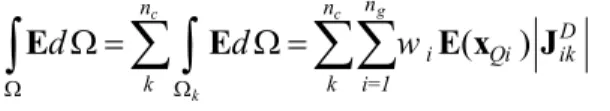
To determine stiffness, mass and force matrices achieved by the meshfree method it is im-portant to implement a suitable numerical scheme to carry out the integrals of Eqs (19). The well-known Gauss quadrature numerical integration approach can be utilized. From the Gauss quadra-ture integration the integral of a function can be evaluated in the specified Gauss pointswith their related weight coefficients. The appropriate number of Gauss points to be used depends upon the complexity of the integrand. A background cells - independent from field nodes - is necessary for numerical integrations of Eqs. (19). Using Gauss quadrature approach to perform the integrations numerically over these cells in general form leads to
( )
g c c k n n n Di Qi ik
k k i=1
d
d
w
E
E
E x
J
(21)where ng is the number of Gauss points in each background cell, wiis the Gauss weighting factor
for the ith Gauss point at xQi (Figure 1) and
D ik
J
is Jacobian matrix for the area integration of the background cell k,at which Gauss point xQi is located.Figure 1: A straight beam represented by a set of field nodes along its neutral axis and background cells.
2.3 Time Integration Scheme
The central difference time integration scheme is used to solve Eq. (18) as an explicit method
2 2 2
1 1 2 1 1
2 t t t t 2 t t
t t
t M C U F K t M U t M C U
(22)
where
t
and t denotes time and time step of integration, respectively. This scheme is stable ifmax
1/
cr
t t
, wheremaxis the largest frequency of the system (Chen et al. 2006). This
condi-kthcell
ithxQ at kthcell
Field nodes
Neutral axis of beam (Ω) Support domain of xQi
tion guarantees the accurate propagation of wave energy along the structure. The Zero initial condi-tions, U0 and U 0at t0are assumed to be implemented as initial displacement and velocity.
2.4 Damage Quantification Based on Wave Propagation for Notched Beams
This section presents how damage extent can be estimated using wave propagation by considering a
uniform Euler–Bernoulli beam with step damage perpendicular to the beam axis with depth Hd.
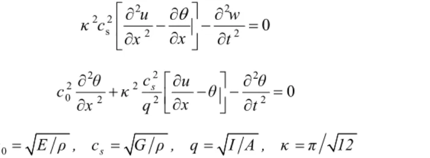
Figure 2 demonstrates the segments of the prescribed rectangular cracked beam. By neglecting the twisting effect and the assumption of the beam axis being the x-axis, the equation of motion for Euler–Bernoulli beam can be expressed in terms of the lateral displacement u(x, t) and the rotation angle θ(x, t) (Doyle 1997, Su et al. 2003)
2 2
2 2
s 2 2 0
u w κ c x x t
(23a)
2
2 2
2 2
0 2 s2 2 0
c u
c κ
x
x q t
(23b)
0 s
c E ρ , c G ρ , q I A , κ π 12 (23c)
where, E, I, A, ρand κ denote the elastic modulus, second moment of area, cross-section area, mass density and shear correction parameter, respectively. By considering of the dispersion relations:
0 i kx t 0 i kx t
u u e , e (24)
the eigen roots (wavenumber) for Eq. (23) can be yielded as
1 2 2 2
2 2
0 0 0
2 2 2 2
0
1 1 1 1 1 2 3 4
2 4
n
s s
c c c
k n
q c
c c , , , ,
(25)
Figure 2: Damage model for quantification based on wave propagation.
1 ikx 2 ikx 3 kx 4 kx i t
u x t ,
A e
A e
A e
A e e (26)where each term corresponds to one of the wave modes depending on their propagating direction and properties: the positively propagating wave (A1), the negatively propagating wave (A2), the
positively growing ringingwave (A3) and the negatively exponentially decaying wave (A4). The
coef-ficient of each term represents the amplitude of each wave component which may be a complex problem.
Interaction between the incident wave and the damage yields to two propagating equations re-sults from Eq. (26) before and after the damage position (referring to Figure 2), denoted with u- and u+, respectively
1 1 1
1 ik x 2 ik x 4 k x i t
ux t,
A e
A e
A e e (27a)2 2
1 ik x 2 k x i t
ux t,
B e
B e e (27b)where the three terms in Eq. (27a) correspond to the incident wave (A1), reflected propagating
wave (A2) and reflected exponentially decaying wave (A4), respectively, while the two terms in Eq.
(27b) are the damage-induced positively propagating wave (B1) and growing attenuating wave (B2),
respectively. The wave components A4 and B2 disappear very quickly due to exponentially
decay-ing. Applying the following continuity and equilibrium conditions yields to the amplitudes of wave components (Kim and Kim 2000)
u x t u x t
u x t u x t
x x
, ,
, , ,
(28)
2 2 3 3
1 2 2 2 1 3 2 3
u x t u x t u x t u x t
EI EI EI EI
x x x x
, , , ,
,
(29)
The reflection ratio can be found as the relation between the magnitude A2 of the reflected wave
and the magnitude A1 of the incident wave
2 4 3 2 2 3 2 4
2 1 1 1 2 1 2 1 2 1 2 1 2 1 2 2 2
2 4 3 2 2 3 2 4
1 1 1 1 2 1 2 1 2 1 2 1 2 1 2 2 2
2
2
2
2
2
2
A
iI k
I I k k
iI I k k
I I k k
iI k
R
A
I k
I I k k
I I k k
I I k k
I k
(30a)3 3
1 12 2 12 d
l H H
l H
I , I (30b)
where l and H are the width and depth of the cross-section of the beam, respectively; while Hd
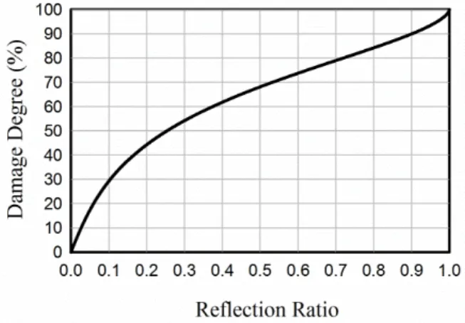
rep-resents the depth of the damage. The reflection ratio is a complex number which indicates that there is a phase shifting relative to the incident wave (Graff 1991). Eq. (30) implies that the depth of damage, Hd, can be determined with a given reflection ratio. Figure 3 represents the absolute
Figure 3: Theoretical relationship between reflection ratio and damage degree.
2.5 Computation of Reflection Ratio Using Hilbert Transform
The Hilbert transform (HT) is useful to the analysis of an inverse problem such as damage assess-ment. The application of HT to the signal provides some additional information about signal con-tent. One of these information is the envelope function which contains important information about the energy of the signal. For an arbitrary time series X(t), the HT is defined as (Sun et al. 2009)
1 XX t H X t dτ
t
(31)
The Hilbert transform performs a 90º phase shift to construct the so-called analytic signal Z(t) as
ei t
Z t X t iH t e t (32)
whose real part is the original signal X(t) itself and imaginary part is its HT. The envelope e(t) and instantaneous phase φ(t) can be expressed by
2 2
e t X t H t (33a)
arctanH t t
X t
(33b)
Therefore, based on HT results, the reflection ratio can be obtained by driving the amplitude of the corresponding energy peak by that of the incident energy peak in the time domain.
3 NUMERICAL ANALYSIS
3.1 Numerical Model
were presented for one-sided step damage, however since this study investigates the 1D beam model as a straight line the mentioned formulation governs the scheme such as Figure 4 where the damage is located in two sides of the x-axis.The field nodes are distributed regularly along the x-axis. In addition, the background cells are introduced with various numbers of Gauss points independent from field nodes. Thehomogeneous beam is located on the spring support at the two ends and its length is 1000 mm. The cross-sectional dimensions are: width 25 mm and height 25 mm and
Young’s modulus and the mass density are equal to 70 GPa and 2700 kg/m3, respectively. Damage
extent is considered as 50% reduction in the height of cross section (Hd) for more clarity of
reflec-tion ratio in captured signal. The corresponding value of reflecreflec-tion ratio for 50% damage extent is equal to 0.2533 based on Figure 3. This damage is located at 700 mm from the left end (Ps) and it
has the length (Ld) equal to 2 mm. The excitation signal is a Hanning-windowed sinusoidal wave
with the central frequency of 250 kHz, which is applied in the first degree of freedom u1 (Figure 5). The output response signal is captured at the point S in location Ps equal to 425 mm. This point
saves the incident and reflected waves from damage position. It is to be noted the damping matrix applies as C M with η=0.02 in Equation (18). Figure 6 shows the benchmark signals of FE wave propagation analysis for undamaged and damaged state including signal's envelope. It is concluded in Figure 6(b) the existence of 50% damage caused reflection ratio nearly equal to 25% corresponds to Figure 3.
Figure 4: Schematic meshfree model of a damaged Euler-Bernoulli beam.
Figure 6: FE output signal in (a) undamaged, (b) damaged.
The main parameters that affects the results of wave propagation in MQ-type HRPIM includes: the number of failed nodes (nf), the dimensionless size of the support domain (αs), shape parameters of MQ (q, αc), the number of polynomials (np) and the total number of Gauss integration points (ng). In this study, first, Gauss points are assumed such as ng 3nf for the stable solution and the prevention of singularity and other parameters are studied under this condition. In the last the ef-fect of the arrangement of ng is investigated independently.
3.2 Study of the Parameters of MQ (αc, q) and Node Density
According to Eq. (13), three parameters in MQ affect the interpolation results, including q, αc and
dc. dc is the characteristic length as the space between two nodes, and it covers the number of field nodes (nf) implicitly. These parameters relate to each other, and independent evaluation of them is not rational. Therefore, Figs. 6-10 represent the contour plot of root mean square error (RMSE) and corresponding percentage error of the reflection ratio. These figures extracted for steps equal to 0.2 for q and αc.The field node density equals to 100, 200, 300, 400 and 500. In this result two terms of polynomials (m=2) are considered for interpolation in Eq. (1) and ng=3000 (three Gauss points on each of 1000 cells that six points are located in damage length) RMSE measures the difference be-tween signals predicted by HRPIM and the signal which is obtained from the benchmark FE model in Figure 6 as
% =
N
m
2100
t t t=1
RMSE
f
f
N
(34)whereftand m t
f
are HRPIM and benchmark signals, respectively, and N is the number of samplingtimes. Also percent error (er) of reflection ratio calculates as
= HRPIM FE 100
r
FE
R -R
e
R (35)
Figure 7: 100 field nodes: (a-1)to(a-4): RMSE for αs=1, 2, 4, 8. (b-1)to(b-4): percentage error
of reflection ratio for αs=1, 2, 4, 8.
Figure 8: 200 field nodes: (a-1)to(a-4): RMSE for αs=1, 2, 4, 8. (b-1)to(b-4): percentage error
of reflection ratio for αs=1, 2, 4, 8.
Figure 9: 300 field nodes: (a-1)to(a-4): RMSE for αs=1, 2, 4, 8. (b-1)to(b-4): percentage error
of reflection ratio for αs=1, 2, 4, 8.
Figure 10: 400 field nodes: (a-1)to(a-4): RMSE for αs=1, 2, 4, 8. (b-1)to(b-4): percentage error
of reflection ratio for αs=1, 2, 4, 8.
* This color bar is related to figures 7 to 11.
Figure 11: 500 field nodes: (a-1)to(a-4): RMSE for αs=1, 2, 4, 8. (b-1) to (b-4): percentage error of reflection ratio for αs=1, 2, 4, 8.
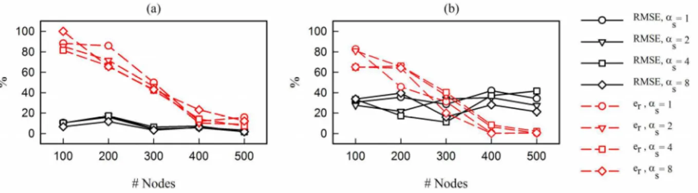
par-ticular the reflection ratio is more sensitive to node density, regardless of the weight of other varia-bles ((b-1) to (b-4) in Figures 7 through 11). Figure 12(a) shows the variation of minimum RMSE of each node density and the corresponding er relative to the node densities while in Figure 12(b) the minimum er and related RMSE is plotted. Both of these figures show the tendency to the least error by increasing of the node numbers. Although in Figure 12(b) the RMSE is stable and er
de-creases. Figure 12 shows that minimum RMSE or minimum er are not dependant to the same
val-ues of (αc,q) and αs. Table 1 compares the results of (αc,q) for different αs in Figure 12. The im-portant point is that the most of the values in Table 1 are in the vicinity of zones which are sensi-tive to any changes (q=0.2, αc=0.2, q=5 and αc=5) and it has relative high errors compared with amounts in the middle range of Figures 7 through 11. It is better we seek the condition that both RMSE and er would be acceptable.
Figure 12: (a) Minimum RMSE and related er (b) Minimum erand related RMSE.
αs 100 nodes 200 nodes 300 nodes 400 nodes 500 nodes
Fig.11(a) Fig.11(b) Fig.11(a) Fig.11(b) Fig.11(a) Fig.11(b) Fig.11(a) Fig.11(b) Fig.11(a) Fig.11(b)
1 (1.6,0.2) (0.4,0.6) (1.0,1.8) (0.8,0.2) (2.8,0.6) (0.8,0.2) (1.6,3.6) (0.2,3.6) (2.0,0.4) (0.6,4.4) 2 (3.0,0.2) (0.8,0.2) (0.6,3.2) (1.0,0.2) (2.4,5.0) (0.8 0.2) (0.4,4.8) (0.2,0.2) (0.2,1.8) (0.2,0.6) 4 (5.0,4.3) (0.2,0.4) (2.4,1.2) (2.4 0.6) (5.0,4.8) (1.0,0.4) (5.0,4.8) (0.2,0.4) (2.4,4.8) (0.2,0.4) 8 (4.0,3.4) (0.2,0.4) (4.8,2.6) (0.2,0.2) (4.6,2.8) (3.6,4.6) (5.0,2.4) (0.2,0.4) (4.2,3.2) (4.6,3.2)
Table 1: Values of (αc,q) for different node density in Figure 12.
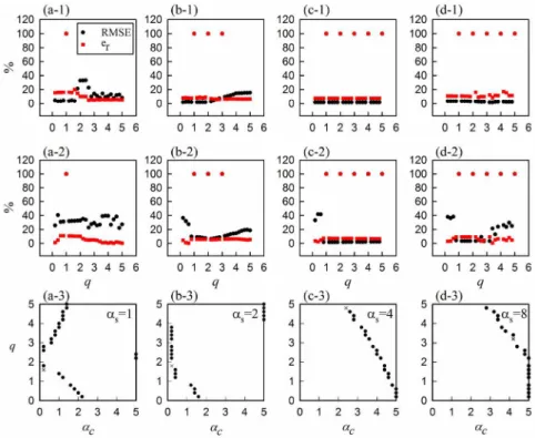
In accordance with Figures 7 through 11, the integer values of q are inappropriate and the anal-ysis would be unstable and singular. However, just q=1 leads to singularity in all of the node densi-tiesfor αs=1. Figure 11 shows that nf =500 has the least error among the other node numbers that has the acceptable errors. Figures 13 (a-1) to (d-2) shows the path of minimum RMSE and er along
q-axis for various αs. There is a good correlation between the minimum RMSE and related er (Fig-ures (a-1) to (d-1)) compared with the other one even for αs=1 which has the significant dispersion between results. It should be noted the results of αs=4 has the constant difference between RMSE and er however it seems αs=2 may lead to the reliable damage quantification.
Equa-tion (33a). Figure 14(a) represents that there is a high-quality agreement among HRPIM and FE envelopes for health beam in such a way the incident and reflected energy of FE and HRPIM are matched. However, HRPIM envelopes with the same parameters lead to lower evaluation of the damage extent in Figure 14(b). It is to be noted that incident waves are coincided, but the reflected signals by damage has lower amplitude. The computed reflection ratios are equal to 0.2025, 0.2305, 0.2345, 0.2308 for αs=1, 2, 4, 8, respectively. Based on these reflection ratios, damage quantification by Figure 3 indicates the extent of damage as 44.62%, 47.71%, 48.12% and 23.08% respectively while the exact value is 50%.
Figure 13: 500 nodes: (a-1)to(d-1) minimum RMSE and related er relative to q for αs=1, 2, 4, 8
(a-2) to (d-2) minimum erand related RMSE for αs=1, 2, 4, 8 (a-3) to (d-3)
distribution of minimum RMSE relative to q (× denotes the minimum value).
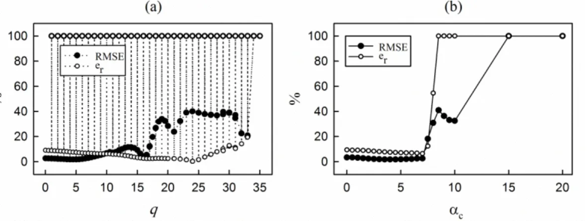
Above analysis studied the comparison of RMSE and er for different αc, αc and q which have the minimum error. Therefore the sensitivity analysis is required for investigation on the effect of each parameter on the other constant value. Figure 15(a) shows RMSE and er for q while αc=2.5 and
αs=4. The initial point of the graphs is q=0.01 and it has the reasonable error. In line with Figure 11, the integer values of q are suffering from the singularity, but even the imperceptible amount (±0.01) less or greater than the specified integer q serves the stability of numerical analysis. It is noticeable the results for two q±0.01 are close to each other. The other noticeable consequence is that the increasing of q leads to the reduction in both of RMSE and er, but from q=4. 99, RMSE increases until q reaches to 9.99 and two graphs are crossover and er surpassed RMSE. Moreover,
q>15 have a propensity to high error, but there is no singularity and the computation remains sta-ble. In this range, reflection ratio and damage quantification have an acceptable evaluation that is due to a shift in HRPIM signal relative to the benchmark FE signal without any change in ampli-tude. By increasing of higher than q=33.99 the analysis is singular.
Figure 15(b) shows the variation of RMSE and er relative to αc when q=2.5 and αs=4. It shows that both RMSE and ertends to low value, however, for αc>7 the unstable results are achieved and quantification of damage cannot be applied.
Figure 15: 500 nodes, RMSE and er relative to (a) q (αc =2.5) (b) αc (q=2.5).
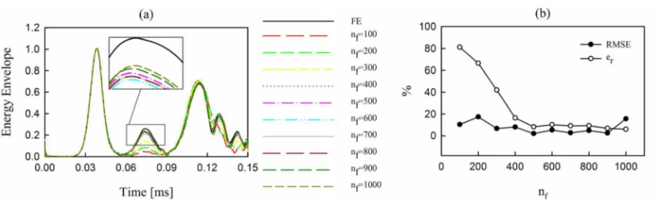
A question that may be raised at this section is that the high density for condition q= 2.5,
Figure 16: The effect of nf (q= 2.5, αc=2.5, αs=4, ng=3000) (a) envelope energy (b) RMSE and er.
3.3 Study of the Size of Support Domain
The number of field nodes that should be used to interpolate and shape function construction re-lates to the size of support domain. This parameter covers the domain around a specific Gauss points and the field nodes located within this domain contribute to interpolate. Figure 17(b) repre-sents as regards αs=1 has improper RMSE equal to 34.2980 but it leads to acceptable er= 9.1219. It is concluded αs=2 assess the reflection ratio a little better than αs=4 however RMSE related to α s=4 is the minimum quantity along αs-axis. Moreover, the increasing of the size of support domain
greater than αs=4 does not lead to better results.
Figure 17: The effect of αs (q= 2.5, αc=2.5, ng=3000) (a) envelope energy (b) RMSE and er.
3.4 Study of the Number of Gauss Points
on the extraction of the damaged system matrices, it seems that the existence of more Gp in dam-aged length may lead to the exact reflection ratio and remarkable coincidence with not only FE signal as an approximated response but also to the analytical response. However, Figure 18 - as the reflected part of the energy envelope - shows that the high ng may not necessarily have the high accuracy. In this figure the number of cells (ncell) is constant as ncell=1000 and ng increases. For set of ng=[3,4,5,6,7,8,9,10] the number of Gp on damage length (Ld=2mm) are [6,8,10,12,14,16,18,20]. It
is notable ng=3 is the best result in comparison with ng=10 which has the minimum RMSE and er. Table 2 represents the results of different patterns of background cells and the number of Gp whereas the all number of Gp distributed in the problem domain is equivalent to 3000. The first point is that the existence of same Gp in damage length (Ld) does not guarantee the same energy
envelope, RMSE and er. On the other hand the high Gp on Ld cannot produce the very accurate
answers. For example, ncell=10 and ng=300 results in 28 Gp in Ld which has the acceptable RMSE
equivalent to 2.5857 but it has low reflection ratio (er=9.5948) even compared to states that there are five Gp on Ld. It is noticeable, the patterns which has seven Gp on Ld (ncell=375, ng=8) and one with 5 points on Ld (ncell=6, ng=500) has the results better than states that there are 6 points on Ld. However, the pattern such as ncell=8, ng=375 produces three Gp on Ld with considerable
reflec-tion ratio error.
Figure 18: 500 nodes (a) reflected energy envelope (b) RMSE and er nodes (q= 2.5, αc=2.5, αs=4, ncell=1000).
ncell ng # Gp on Ld RMSE er ncell ng # Gp on Ld RMSE er
3000 1 6 2.0902 7.2083 1 3000 4 2.4095 7.7646 1500 2 6 2.1530 8.3825 2 1500 4 2.3119 6.5414 1000 3 6 2.0605 8.2291 3 1000 6 2.5696 10.8060
750 4 6 2.7824 7.8160 4 750 5 1.8218 7.6374 600 5 6 3.5825 12.2180 5 600 4 1.9092 5.0506 500 6 6 1.7989 10.8070 6 500 5 2.4417 4.6012 375 8 7 2.2835 4.7081 8 375 3 3.7753 20.5920 300 10 6 2.5732 5.6499 10 300 28 2.5885 9.5948
3.5 Study of the Number of Polynomial Terms
Equation (1) is the formulation of pure HRPIM which is augmented with m polynomial basis
func-tions. Essentially, adding polynomials is not necessary always; however it can ensure the inverse of matrix G in Equation (7), consistency, improvement of accuracy and stability of problem. Figure 19
shows the results of wave propagation relative to the number of polynomial terms (m). In this
study, pure HRPIM (m=0) is stable and nonsingular. But Figure 19(b) shows that increasing of m
leads to accurate results with slight drop in RMSE and er. Although, for m=0, RMSE and er are equal to 2.7865 and 8.7022, respectively whereas m=1 evaluates RMSE=2.8071 and er=8.7595. The notable point is the instability of signals and envelopes for m>5. In this form, problem is not singu-lar but detection of reflected wave is not possible as shown in Figure 19(a) for m=6, 7.
Figure 19: The effect of the number of polynomial terms (m) (nf=500, q= 2.5, αc=2.5, αs=4, ng=3000) (a) envelope energy (b) RMSE and er.
4 RESULTS
This paper investigated the numerical modeling of wave propagation for damage quantification in Euler-Bernoulli beam using Hermite RPIM by considering MQ-type RBF. The damage was consid-ered as a reduction in the depth of the cross section in the specific position. Extraction of the rela-tion between the reflecrela-tion ratio and damage extent was utilized as a tool for the assessment of the capability of HRPIM. In addition to the reflection ratio, RMSE between the captured signals of HRPIM and FE models were determined for the sensitivity analysis of results relative to the effec-tive parameters. Number of field nodes, shape parameters of MQ, the size of support domain, the number of Gauss points and the number of polynomial terms were the main effective variables. This study can draw the following conclusions:
(a) The number of field nodes is the most significant parameter for accurate wave propagation modeling using HRPIM. It is concluded to achieve an accurate results, the consideration of a high density of field node is required.
(b) MQ is a suitable RBF for HRPIM and wave propagation; however, care must be taken in
sensitive to high value of q and it is better q should be less than 15. There is such re-striction about other shape parameter αc and low value is preferred for this quantity.
(c) It is better to consider αs<5 for the size of support domain. Greater values make high RMSE and reflection ratio error.
(d) Gauss quadrature points are important for determination of support domain and to derive
the system matrices. This study investigated different patterns of Gauss points in such a way the total number of Gauss points is constant. It is concluded the existence of extra Gauss points in damage region does not guarantee the more accurate reflected wave. In general, the number of Gauss points is assumed as ng 3nf for the stable solution and to
prevent the singularity.
(e) Pure HRPIM without any polynomial terms is acceptable and there is no singularity in so-lution but considering a few terms improve the accuracy; however more terms make the problem unstable.
References
Bozkurt, O. Y., B. Kanber and M. Z. AŞIk (2013). Assessment of RPIM shape parameters for solution accuracy of 2D geometrically nonlinear problems. International Journal of Computational Methods 10(03): 1350003.
Buhmann, M. D. (2003). Radial basis function: theory and implementation, Cambridge University Press.
Chakraborty, A., D. R. Mahapatra and S. Gopalakrishnan (2002). Finite element analysis of free vibration and wave propagation in asymmetric composite beams with structural discontinuities. Composite Structures 55: 23-36.
Chen, Y., J. Lee and A. Eskandarian (2006). Meshless methods in solid mechanics, Springer.
Cui, X., G. Liu and G. Li (2009). A smoothed Hermite radial point interpolation method for thin plate analysis. Archive of Applied Mechanics 81(1): 1-18.
Das, S. and T. Kundu (2009). Mesh-free Modeling of Ultrasonic Wave Fields in Damaged Layered Half-spaces. Structural Health Monitoring 8(5): 369-379.
Dehghan, M. and A. Shokri (2009). Numerical solution of the nonlinear Klein–Gordon equation using radial basis functions. Journal of Computational and Applied Mathematics 230(2): 400–410.
Doyle, J. F. (1997). Wave propagation in structures: spectral analysis using fast discrete Fourier transforms, Spring-er; 2nd edition.
Fedoseyev, A. I., M. J. Friedman and E. J. Kansa (2002). Improved multiquadric method for elliptic partial differen-tial equations via PDE collocation on the boundary. Computers & Mathematics with Applications 43(3-5): 439–455. Fornberg, B. and G. Wright (2004). Stable computation of multiquadric interpolants for all values of the shape pa-rameter. Computers & Mathematics with Applications 48(5-6): 853-867.
Franke, R. (1982). Scattered data interpolation: test of some methods. Mathematics of Computation 38: 181-200. Gao, L., K. Liu and Y. Liu (2007). A meshless method for stress-wave propagation in anisotropic and cracked media. International Journal of Engineering Science 45(2-8): 601-616.
Ghaffarzadeh, H. and A. Mansouri (2013). Numerical modeling of wave propagation using RBF-based meshless method. Proc. of the Intl. Conf. on Future Trends in Structural, Civil, Environmental and Mechanical Engineering-FTSCEM, Bangkok, Thailand, IRED.
Graff, K. F. (1991). Wave motion in elastic solids, Dover Publications.
Hon, Y. C. and Z. M. Wu (2000). A quasi-interpolation method for solving stiff ordinary differential equations. In-ternational Journal for Numerical Methods in Engineering 48: 1187–1197.
Kanber, B., Ö. Y. Bozkurt and A. Erklig (2013). Investigation of RPIM Shape Parameter Effects on the Solution Accuracy of 2D Elastoplastic Problems. International Journal for Computational Methods in Engineering Science and Mechanics 14(4): 354-366.
Kansa, E. J. (1990a). Multiquadrics—A scattered data approximation scheme with applications to computational fluid-dynamics—I surface approximations and partial derivative estimates. Computers & Mathematics with Applica-tions 19(8-9): 127-145.
Kansa, E. J. (1990b). Multiquadrics—A scattered data approximation scheme with applications to computational fluid-dynamics—II solutions to parabolic, hyperbolic and elliptic partial differential equations. Computers & Mathe-matics with Applications 19(8-9): 147–161.
Keramat, A. and A. Ahmadi (2012). Axial wave propagation in viscoelastic bars using a new finite-element-based method. Journal of Engineering Mathematics 77(1): 105-117.
Kim, Y. Y. and E. H. Kim (2000). A new damage detection method based wavelet transform. Proceedings of 18th IMAC, San Antonio, Texas, USA.
Kudela, P., M. Krawczuk and W. Ostachowicz (2007). Wave propagation modelling in 1D structures using spectral finite elements. Journal of Sound and Vibration 300(1-2): 88-100.
Lazzaro, D. and L. B. Montefusco (2002). Radial basis functions for the multivariate interpolation of large scattered data sets. Journal of Computational and Applied Mathematics 140: 521–536.
Li, H. and S. S. Mulay (2013). Meshless methods and their numerical properties, CRC Press. Li, S. and W. K. Liu (2007). Meshfree particle methods, Springer.
Liew, K. M. and X. L. Chen (2004). Buckling of rectangular Mindlin plates subjected to partial in-plane edge loads using the radial point interpolation method. International Journal of Solids and Structures 41(5-6): 1677-1695. Liew, K. M. and X. L. Chen (2004). Mesh-free radial point interpolation method for the buckling analysis of Mindlin plates subjected to in-plane point loads. International Journal for Numerical Methods in Engineering 60(11): 1861-1877.
Liu, G. R. (2010). Mesh Free Methods Moving Beyond the Finite Element Method, CRC Press.
Liu, G. R. and Y. T. Gu (2001). A point interpolation method for two dimensional solids. International Journal for Numerical Methods in Engineering 50(4): 937-951.
Liu, G. R., G. Y. Zhang, Y. T. Gu and Y. Y. Wang (2005). A meshfree radial point interpolation method (RPIM) for three-dimensional solids. Computational Mechanics 36(6): 421-430.
Liu, G. R., X. Zhao, K. Y. Dai, Z. H. Zhong, G. Y. Li and X. Han (2008). Static and free vibration analysis of lami-nated composite plates using the conforming radial point interpolation method. Composites Science and Technology 68(2): 354-366.
Liu, G. R., Y. Li and Y. Dai (2006). A linearly conforming radial point interpolation method for solid mechanics problems. International Journal of Computational Methods 3(4): 401–428.
Liu, Y., Y. C. Hon and K. M. Liew (2006). A meshfree Hermite-type radial point interpolation method for Kirchhoff plate problems. International Journal for Numerical Methods in Engineering 66(7): 1153-1178.
Mitra, M. and S. Gopalakrishnan (2005). Spectrally formulated wavelet finite element for wave propagation and impact force identification in connected 1-D waveguides. International Journal of Solids and Structures 42(16-17): 4695-4721.
Moser, F., L. J. Jacobs and J. Qu (1999). Modeling elastic wave propagation in waveguides with the finite element method. NDT&E International 32: 225–234.
Rippa, S. (1999). An algorithm for selecting a good value for the parameter c in radial basis function interpolation. Advances in Computational Mathematics 11: 193–210.
Su, Z., L. Ye, X. Bu, X. Wang and Y. W. Mai (2003). Quantitative Assessment of Damage in a Structural Beam Based on Wave Propagation by Impact Excitation. Structural Health Monitoring. 2(1): 27-40.
Sun, K., G. Meng, F. Li, L. Ye and Y. Lu (2009). Damage Identification in Thick Steel Beam Based on Guided Ultrasonic Waves. Journal of Intelligent Material Systems and Structures 21(3): 225-232.
Tiago, C. M. and V. M. A. Leitão (2006). Application of radial basis functions to linear and nonlinear structural analysis problems. Computers & Mathematics with Applications 51(8): 1311-1334.
Wang, J. G. and G. R. Liu (2000). Radial point interpolation method for elastoplastic problems. Proceedings of the First International Conference on Structural Stability and Dynamics, Taipei, Taiwan.
Wang, J. G. and G. R. Liu (2002). A point interpolation meshless method based on radial basis functions. Interna-tional Journal for Numerical Methods in Engineering 54(11): 1623-1648.
Wang, J. G. and G. R. Liu (2002). On the optimal shape parameters of radial basis functions used for 2-D meshless methods. Computer Methods in Applied Mechanics and Engineering 191: 2611–2630.
Wang, J. G., G. R. Liu and P. Lin (2002). Numerical analysis of Biot's consolidation process by radial point interpo-lation method. International Journal of Solids and Structures 39(6): 1557–1573.
Wen, P. H. (2010). Meshless local Petrov–Galerkin (MLPG) method for wave propagation in 3D poroelastic solids. Engineering Analysis with Boundary Elements 34(4): 315-323.
Wendland H. (2010). Scattered data approximation. Cambridge University Press.
Wu, Z. (1992). Hermite-Birkhoff interpolation of scattered data by radial basis function. Application Theory and its Applications 8: 1-10.
Yim, H. and Y. Sohn (2000). Numerical simulation and visualization of elastic waves using mass-spring lattice model. IEEE transactions on ultrasonics, ferroelectrics, and frequency control 47(3): 549-558.
Zhang, G. M. and R. C. Batra (2004). Modified smoothed particle hydrodynamics method and its application to transient problems. Computational Mechanics 34(2).