Computing the Acoustic Field of a Radiating
Cavity by the Boundary Element - Rayleigh
Integral Method (BERIM)
Stephen Kirkup and Ambrose Thompson
Abstract—This paper describes the Fortran subrou-tine BERIM3 that delivers a computational solution to the acoustic field both within and outside of a cav-ity with one opening into the exterior domain. The mathematical model is based on coupling the usual di-rect boundary integral equation for the interior region to the Rayleigh integral for the mouth of the domain and the exterior region. The usual boundary element method (BEM) and Rayleigh integral method (RIM) systems of equations are coupled through the appli-cation of continuity at the mouth of the cavity. The method is applied to a horn loudspeaker.
Keywords: boundary element method, loudspeaker, acoustics, sound, vibration, cavity
1
Introduction
Methods based on integral equations, or boundary ele-ment methods (BEMs) have played an important role in many areas of science and engineering. Boundary Ele-ment Methods have been applied in acoustics for many decades. In this manual, a method and computer code (BERIM3) are developed for solving the acoustics of an open cavity. The acoustic domain is the connected region both within and exterior to the cavity. There are at least three approaches to solving the open cavity problem us-ing integral equation techniques. One method is to treat it as an exterior problem and apply the BEM by wrap-ping elements both around the exterior and the interior cavity walls, for example by using the AEBEM* meth-ods Kirkup [9]. A second method is to close the cavity and couple boundary integral equation reformulations of the interior and exterior regions across the openings (eg coupling the AIBEM* and AEBEM* programs of Kirkup [9]). An alternative method is to close the (one) open-ing of the cavity and couple the interior boundary inte-gral equation with the Rayleigh inteinte-gral (ie coupling the
∗Stephen Kirkup, Engineering Research Group, East Lancs
In-stitute of Higher Education, Blackburn, Lancashire, UK Email: [email protected]. Ambrose Thompson, Martin Audio, High Wycombe, Email [email protected]. The first au-thor would like to thank the partial sponsorship of the New Engi-neering Fellowships scheme (www.neweng.org).
AIBEM* and ARIM* methods of Kirkup [9], [8]) . It is this this third method that is considered in this paper.
Boundary element methods can be applied to acoustic problems in their generality [9]. They can be applied to either of the areas of engine or machine noise (for example [2]) or to audio [1], [11]. In this paper we will briefly consider audio applications.
Figure 1. The cavity opening on to a baffle.
The physical problem is illustrated by Figure 1. The acoustic domain is the cavity and the half-space beyond the mouth. The baffle is rigid and perfectly reflecting. This model can be applied to a range of acoustic cavity problems. In any practical problem the baffle must be finite. Even if there is no baffle, at least the continuity in the acoustic field is maintained across the mouth and the model can still be applied with due care. The BERIM method can be applied in the usual two dimensional, three dimensional and axisymmetric domains. BERIM3 is an implementation of the methods required for general three dimensional problem.
In this paper the integral equation formulations that form the basis of the BERIM method are stated. The meth-ods are developed through applying collocation to the integral equations and coupling them across the open-ing. The resulting linear systems of equations are stated. The BERIM method for solving general three dimen-sional problems is implemented in the Fortran subroutine BERIM3. This subroutine is described and results from its typical application to a horn loudspeaker are validated through comparison with measurement.
2
Modelling
The acoustic radiation model consists of a cavity with interior surface S’. In order to work towards a solution, the surface S’ is completed using a flat fictitious surface over the opening Π, giving an interior region D and an exterior region E. The interior field and the exterior field are then reformulated as integral equations and the for-mulae are coupled. The acoustic domain is modelled as shown in figure 1, however the baffle is now presumed to be infinite and perfectly reflecting. The two formula-tions are coupled across Π through presuming continuity of potential (sound pressure) and its derivative.
2.1
Mathematical Model
The equation that we need to solve at each wavenumber (or frequency) is the Helmholtz (reduced wave) equation
∇2
ϕ(p) +k2ϕ(p) = 0 .
whereϕis the (time-independent) velocity potential. See Kirkup [7] for the derivation of this method. In general, let it be assumed that we have a Robin condition on the cavity surface of the form
a(p)ϕ(p) +b(p)v(p) =f(p) (p∈S′) (1)
where v(p) = ∂np∂ϕ with f(p) given for p ∈ Π and np
is the unit normal to the surface at p. (In this report we will be mainly concerned with the Neumann problem (a(p) = 0,b(p) = 1 forp∈Π).
The time-independent sound pressure can easily be found from the velocity potential:
P(p) =iρωϕ(p) (p∈Π∪E). (2)
2.2
Rayleigh Integral Formulation
The Rayleigh integral formulation is used in the exterior region. In brief, it relates the velocity potentialϕ(p) at a pointpin the exteriorE, on the opening Π, or on the baffle to the normal velocityv on the opening Π. (Note that in the standard method the opening is a vibrating panel.)
In the standard integral operator notation used in inte-gral equation methods (see Kirkup [6] for example) the Rayleigh integral is as follows,
ϕ(p) =−2{Lkv}Π(p) (p∈Π∪E). (3)
In equation (3) the operatorLk is defined by
{Lkζ}Γ(p)≡
Γ
Gk(p,q)ζ(q)dSq (p∈Γ∪E), (4)
where Gk(p,q) is a free-space Greens function for the
Helmholtz equation and Γ represents the whole or part of the opening. In this document the Green’s function is defined as follows
Gk(p,q) =
1 4π
eikr
r (k∈R
+
), (5)
where r =|r|, r= p−q, R+ is the set of positive real
numbers andiis the unit imaginary number. The Green’s function (5) also satisfies the Sommerfeld radiation con-dition, ensuring that all scattered and radiated waves are outgoing in the farfield.
2.3
Interior Helmholtz Integral Equation
Formulation
The application of Green’s second theorem to the Helmholtz equation gives the following equations:
{Mkϕ}S′Π(p) +ϕ(p) ={Lkv}S′Π(p) (p∈D),
(6)
{Mkϕ}S′Π(p) +
1 2ϕ(p) =
{Lkv}S′Π(p) (p∈S′
Π). (7)
The operator Lk is defined by (4), but with Γ
respre-senting the whole or part ofS′
Π. The operator Mk is
defined as follows
{Mkζ}Γ(p)≡
Γ
∂Gk
∂nq
(p,q)ζ(q)dSq . (8)
Note that the normals to the boundary are taken to be in the outward direction.
Dividing the inner surface from the mouth allows us to write (9) and (7) as follows:
{Mkϕ}S′(p) +{Mkϕ}Π(p) +ϕ(p) =
{Lkv}S′(p) +{Lkv}Π(p) (p∈D), (9)
{Mkϕ}S′(p) +{Mkϕ}Π(p) +
1 2ϕ(p) =
{Lkv}S′(p) +{Lkv}Π(p) (p∈S′
3
Boundary Element - Rayleigh Integral
Method
Approximations to the properties of the acoustic medium can be found through applying collocation to the integral equations (7) and (3). This requires us to represent the surfaceS′ and the opening Π by a set of panels and the
functions ϕ and v on S′ and Π by constants on each
panel. The equations (7) and (3) can now be written as linear systems of equations and through applying conti-nuity inϕandv on Π the system can be represented by one matrix-vector equation where the matrix is square. Through solving this equation, approximations toϕand vare obtained onS′ and Π. By substituting the
approx-imations for ϕ and v into the relevant equation above, acoustic properties can be obtained in the interior cavity or in the exterior field.
3.1
Representation of the Interior Surface
and the Opening
In order that the resulting computational method is ap-plicable to a class or arbitrary openings there must be a facility for representing the interior surface and the open-ing as a set of panels. For example a set of triangles can be used to approximate a the interior surface and an opening of arbitrary shape. Thus we may write
Π≈Π =˜
m
1
∆jΠ˜ , (11)
S′≈S˜′=
n
1
∆jS˜′ , (12)
where each ∆jS˜′ and ∆jΠ is a triangle.˜
3.2
Collocation
Let us first apply collocation in the most general sense. The normal velocity on ˜S′and ˜Π is expressed in the form
˜ v(q)≈
m+n
j=1
v(pj) ˜χj(q) = m+n
j=1
vjχ˜j(q) (q∈Π) (13)˜
where ˜χ1, ˜χ2, ..., ˜χm+nare basis functions with the usual
properties:
˜
χi(pj) =δij ,
m+n
j=1
˜
χj(q) = 1 (q∈Π)˜
andvj=v(pj), the velocity at thejth collocation point.
The replacement of (part of) the true surface or opening Γ by ˜Γ and the substitution of the approximation (13) allows us to write
{Lkµ}Γ≈ {Lkµ˜}˜Γ=
{Lk m+n
j=1
µ(pj) ˜χj}Γ˜(p) = m+n
j=1
µj{Lkχ˜j}Γ˜(p). (14)
A similar discretisation can be applied to theMk
opera-tor.
In the BERIM3 method, the surface functions are approx-imated by a constant on each triangle. Hence the basis functions are the sequence of functions that are zero on all but one triangle in turn. In summary the relevant operators can be written as follows:
{Lkµ}Γ(p)≈ m+n
j=1
µj{Lk˜1}∆j(p). (15)
{Mkµ}Γ(p)≈ m+n
j=1
µj{Mk˜1}∆j(p). (16)
where ˜1 represents the unit function and ∆j represents
the jth triangle. Details on the methods employed for evaluating the {Lk˜1}∆j(p) and {Mk˜1}∆j(p) values are
given in Kirkup [6], [9].
If in equations (15) and (16) p takes the value of the collocation points then for example for (15):
{Lkµ}Γ(pi)≈ m+n
j=1
µj{Lk˜1}∆j(pi), (17)
and similarly for (16). For each triangle ∆j and each
col-location pointpi in (17) {Lk˜1}∆j(pi) can be evaluated,
so that we have a matrix of values. Let us define the matrix
[Lk]ij={Lk˜1}∆j(pi), (18)
and similarly forMk.
3.3
Equivalent Linear System of Equations
Making substitutions of the form (17), (18) in the integral equations (3) and (10) gives
ϕΠ=−2[Lk]ΠΠvΠ , (19)
where the subscript Π indicates that the discrete operator and functions are considered on the approximate opening Π′ (the prime is dropped for clarity). For the integral
equation (10) the following equation is obtained forp∈ S′
([Mk]SS+
1
2[I]SS)ϕS+[Mk]SΠϕΠ= [Lk]SSvS+[Lk]SΠvΠ ,
(20) and the following forp∈Π′
[Mk]ΠSϕS+([Mk]ΠΠ+
1
2[I]ΠΠ)ϕΠ= [Lk]SΠvΠ+[Lk]ΠΠvΠ .
Bringing together equations (19)-(21) along with the dis-crete form of the boundary condition (1),
[Db]SSϕS+ [Mk]SSvS = 0S ,
gives the following linear system of equations:
⎡
⎢ ⎣
[Da]SS [Db]SS [0]SΠ [0]SΠ [Mk]SS+12[I]SS −[Lk]SS [Mk]SΠ −[Lk]SΠ
[Mk]ΠS −[Lk]ΠS [Mk]ΠΠ+12[I]ΠΠ −[Lk]ΠΠ
[0]ΠS [0]ΠS 2[Lk]ΠΠ [I]ΠΠ
⎤
⎥ ⎦
×
⎡
⎢ ⎣
vS ϕ
S vΠ ϕ
Π
⎤
⎥
⎦=
⎡
⎢ ⎣
fS
0S
0Π 0Π
⎤
⎥
⎦ . (22)
The linear system of equations is (2n+2m)x(2n+2m) and it can be solved using standard direct or iterative meth-ods. The matrix can be simplified in the case of a Neu-mann or Dirichlet boundary condition, in which cases the matrix is (n+2m)x(n+2m).
4
Implementation of BERIM3
In this section an implementation of the boundary ele-ment - Rayleigh Integral method in 3D (BERIM3) is de-scribed. The cavity and opening may be of any shape and is assumed to be discretised into a set of planar triangles. The boundary condition distribution on the opening is described simply by its value at the centroids of the tri-angles, the interpolation points. The basis functionsχ1,
χ2, ...,χnare the constant functions;χj, taking the value
of unity on the jth panel and zero on the remainder of the opening. The pointsp1,p2, ... pn are the centroids
of the triangular elements;
{Lkχj}Π˜ ={Lke}∆ ˜Πj
whereeis the unit functione(p) = 1.
As input, the subroutine accepts a description of the ge-ometry of the opening (made up of triangles), the co-ordinates of selected points in the exterior (where the sound pressure is required), the wavenumbers under con-sideration and a description of the boundary condition at each wavenumber. As output, the subroutine gives, for each wavenumber, the acoustic intensity at the vertices of the triangles that make up the approximate opening, the sound power, the radiation ratio and the sound pressure at the prescribed exterior points.
5
Application to a horn loudspeaker
In this section we compare the computed with measured results for a typical horn loudspeaker.
In order to apply BERIM3 to the horn loudspeaker first the 3D solid model is generated automatically from a set
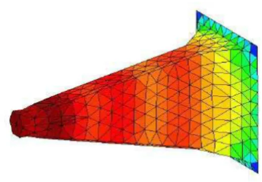
of around 10 parameters. This is then introduced into the popular GID pre/post processor where a triangulation of the interior surface and mouth is made and subsequently solved. A typical GID post process mesh is shown in fig-ure 2. A velocity of 1m/s was set at the throat (assumed to be flat) and zero everywhere else. In order to mitigate the numerical effects of the sudden change in boundary conditions where the cavity surface meets the mouth, a small flange was added. A description of each calculation can be found in Table 1, where number of elements and approximate running time on a AMD2200 PC platform are given.
Figure 2. Typical BERIM3 mesh showing surface SPL at 3kHz.
Table 1. Timing of Computations
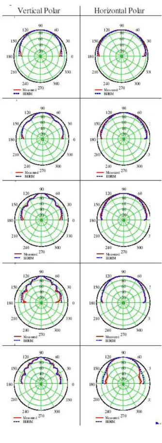
The sound pressure is observed on polar paths of 1m ra-dius. The results from BERIM3 are compared with mea-sured results in Figure 3, showing polar plots of the sound pressure level (spl) in the vertical and horizontal polar plane and an illustration of the mouth velocity ampli-tude for 3,6,9,12,and 15kHz. The popular GID pre/post processor was used to mesh and display the results.
6
Test Problem
Figure 3a. Polar plots of the sound pressure level (spl) in the vertical and horizontal polar plane 3,6,9,12,and
15kHz.
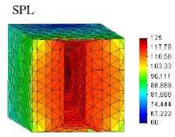
Fig 5. Mesh, showing SPL values at 3kHz.
Fig 6. Horizontal and vertical polar plots at 3kHz.
7
Concluding Discussion
For a structure such as a horn loudspeaker, which con-sists of a cavity (the horn) opening out on to a plane, the Boundary Element Rayleigh Integral Method (BERIM) seems most applicable. In Figure 2 it is shown that BERIM requires a mesh of the interior surface and open-ing plane alone whereas the application of the bound-ary element method (BEM) to the same problem requires considerably more elements. BERIM3 can be compared with the BEM by considering the results in Figure 6, the 3KHz plot in figure 3 and table 1a; similare results are obtained but BERIM3 reduces the meshing required and typically uses an order of magnitude less computer time than the straightforward BEM.
The results in Figure 3 generally show good agreement between computed and measured results, there are a number of other points. BERIM3 seems to give better agreement with measured than the BEM in the forward field, however, near the baffle the BEM has more agree-ment. The proposed reason for this is that the BEM ac-curately meshes the baffle whereas BERIM assumes and infinite baffle; BERIM3 gives more support to the wider field than the true finite baffle.
In general the lobes in the sound field are captured in the results from BERIM3. There is only significant drift in the horizontal polar at 15kHz: this would probably benefit from a further refinement in the mesh. In general BERIM3 is a powerful tool for the simulation of the sound field of a horn loudspeaker; returning results for a given problem and given frequency within a few minutes at low and medium frequencies on a typical modern PC.
References
[1] K. J. Bastyr, D. E. Capone (2003). On the Acoustic Radiation from a Loudspeaker’s Cabinet, J. of the Audio Engineering Society,51(4), 234-243.
[2] M. Furlan, M. Boltezar (2003). The Boundary Ele-ment Method in Acoustics - an Example of Evalu-ating the Sound Field of a DC Electric Motor. J. of Mech Eng,50(2), 115-128.
www.fs.uni-lj.si/sv/English/2004/2/sv-02-an.pdf
[3] E.R.Geddes (1993). Sound Radiation from Acoustic AperturesJ. of the Audio Engineering Society41(4) 214-230.
[4] D. J. Henwood (1993). The Boundary Element Method and Horn Design,J. of the Audio Engineer-ing Society,41(6), 485-496.
[5] S. M. Kirkup (1994). Computational Solution of the Acoustic Field Surrounding a Baffled Panel by the Rayleigh Integral Method,Applied Mathematical Modelling,18, 403-407.
[6] S. M. Kirkup (1998). Fortran Codes for Computing the Discrete Helmholtz Integral Operators,Advances in Computational Mathematics,9, (1998) 391-409.
[7] S. M. Kirkup and A. Thompson (2007). Acous-tic Field of a Horn Loudspeaker Simulation by the Boundary Element Rayleigh Integral Method, Report AR-07-03, East Lancashire Insti-tute,www.elihe.ac.uk/research.
[8] S. M. Kirkup (2007) ARIM3 and BERIM3 manual and codes. www.boundary-element-method.com/acoustics.
[9] S. M. Kirkup (2007).The Boundary Element Method in Acoustics,www.boundary-element-method.com
[10] Martin Audio (2007) Website Historical and Prod-uct informationwww.martinaudio.com
[11] J. Vanderkooy and D. J. Henwood (2006). Polar plots at low frequencies: The acoustic centre,Audio Engineering Society convention paper, 6784, 120th Convention, Paris, France.