Abstract
Due to their robustness in handling the inherent singularity diffi-culties associated with crack analysis, mesh-reduction methods present an avalanche of formulations in the literature which, some-times, entails modifications to their conventional/standard forms for better results. Although such formulations provide a pool of alternative choices to the analyst, increase in their number requires some relative assessment between them in order to guarantee opti-mum choice of analysis tool. The present study assesses the ap-plicability and relative performance of three such mesh-reduction methods, namely the radial basis function (RBF) method, the boundary element method (BEM), and the method of fundamental solution (MFS) for mode III crack analysis. In order to have a common ground for performance comparison, these methods are, first, tested in their most basic forms and simplest conventional formulations possible. Failure of some of them to provide reliable results calls for some enrichments. Yet, unless where necessary, efforts are made to ensure that unnecessary computationally expen-sive formulations are avoided. Consequently, the BEM formulation is not altered in any way, and modifications to both the RBF and MFS are limited to enrichment by the addition of, at most, one singular term and/or the domain-decomposition technique. Verifi-cation is achieved using the literature results and/or those obtained by FEM in this study. Summary of the relative advantages and limitations of the methods for mode III crack analysis is given to serve as a yard-stick based on which the choice of one over the others may be influenced.
Keywords
Mode III cracks, crack-tip singularity, radial basis function, boundary element method, method of fundamental solution, enriched formulation.
Relative Performance of Three Mesh-Reduction Methods
in Predicting Mode III Crack-Tip Singularity
Faisal M. Mukhtar a
a Department of Civil and
Environmen-tal Engineering, King Fahd University of Petroleum & Minerals, 31261, Dhahran, Saudi Arabia.
Email: [email protected]
http://dx.doi.org/10.1590/1679-78253656
1 INTRODUCTION
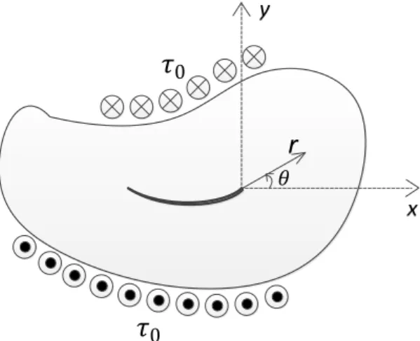
Analysis of cracks in solids is an essential aspect useful for various applications aimed at designing parts against fracture and for life prediction of engineering components. The stress field in the vicin-ity of the crack tip governs the crack growth and, hence, behavior of the crack-tip-field stresses is very essential in fracture mechanics. A crack is made of disjoined upper and lower faces, where the crack front is the common joint between the crack faces. Once subjected to externally applied loads (remote or at the crack surfaces), a cracked solid exhibits any of the three major fracture modes (Mode I, Mode II or Mode III) or their combinations depending on the loading pattern. As shown in Fig. 1, a typical case of mode III is a consequence of subjecting a cracked body to an anti-plane
shear τ0. This loading condition is also referred to as the tearing mode. In order to have an idea
about the extent of stress singularity at a crack tip, the stress intensity factor (SIF) is defined (Ir-win, 1958). This parameter provides a very useful information that helps in characterizing the state of stress near the crack tip due to remote loading.
Figure 1: Illustration of mode III loading condition in an arbitrary shaped cracked body.
There exists a number of analytical solutions for mode III crack problems. Some of these include use of Westergaard stress functions by Sih (1965), the Fourier transform and Fourier series by (Zhang, 1987; Zhang, 1988; Zhang, 1989; Ma, 1988; Ma, 1989; Ma and Zhang, 1991), perturbation procedures by (Chiang, 1987) and the technique for Hilbert problems and Cauchy integrals to solve the problem formulated by representing the internal stresses and the normal displacement by com-plex holomorphic functions by (Vroonhoven, 1995).
differ-ential quadrature element method, which is similar to the FEM in principle, has been used by Liao et al. (2015) for the analysis of mode III cracks’ SIF. Two regions are defined in the approach: A near field circular complementary energy region with stresses as the variables, and a far field poten-tial energy region with displacements as the variables. Coarse mesh sizes are sufficient to achieve the desired accuracy due to the fact that the method employs mathematical discretization rather than geometrical discretization.
FEM requires both the domain and boundary of the problem to be meshed, and the denser the
mesh, the more accurate the solution is (except at points of stress singularities, such as r = 0 in Fig.
1) which results in high computational and memory demand. In addition, the need for re-meshing in FEM is another aspect considered to be time-consuming and bound to result in some errors. One of the best ways to avoid such computational demand and complexities associated with the FEM is the use of mesh-reduction techniques. Consequently, quite a number of such methods applied for fracture analysis are available. Such techniques, including the BEM (Brebbia, 1989) and/or its vari-ances, are very popular techniques with a record of success for mode III crack problems. For exam-ple, Xanthis et al. (1981) presented a form of the boundary integral equation method, and provided a number of approaches for computing SIF for cracked bodies governed by mode III condition. Ap-plication of the boundary integral equation method has been made by Paulino et al. (1993) for an arbitrary shaped body containing a curved crack under mode III loading condition. Discretization of the cut-out boundary was eliminated by incorporating the effect of the crack on the stress field in an augmented kernel. Accurate closed form solution of the SIF at each crack tip is obtained by con-ducting asymptotic analysis. Another formulation of integral equation method for mode III crack problems capable of tackling both smooth and kinked cracks has been reported by Liu and Altiero (1992). Singular integral equation method have also been applied to study Zener-Stroh crack prob-lems loaded in anti-plane mode by Chen and Lin (2007).
cracks, by Chen et al. (1995) and Chen and Chen (2000). BEM and/or its variants have also proved successful when applied to cracked anisotropic or non-homogeneous bodies under anti-plane shear mode such as in the work reported by Ang (1999) and Sun et al. (2003).
A further reduction in the computational efforts can be realized with the use of a sub-class of mesh-reduction methods, the so-called truly meshless methods. Use of element-based discretization is completely eliminated in these methods. A popular approach under this category is the colloca-tion method whose applicacolloca-tion is well established for mode III fracture. For example, displacement functions for crack problems in finite body under anti-plane shear loading have been proposed by Yuanhan (1992) and Yuanhan (1993) for edge and internal cracks, respectively. In both cases, cal-culations of the SIFs have been achieved using the boundary collocation method which yields accu-rate results that compares favorably with those from other sources. Another successful application of the same method to a cracked finite orthotropic plate loaded in anti-plane mode is reported by Wang et al. (1992).
Another technique by collocation using the fundamental solution, popularly known as the meth-od of fundamental solution (MFS) (Kupradze and Aleksidze, 1964), is devised to circumvent the integration needed along the boundary in BEM. The MFS does not require any integration even at the boundary as is the case with BEM. The MFS, however, requires that some virtual boundary be defined over which the source points are placed in order to avoid singularity in the solution. The offset distance to the virtual boundary becomes an issue when MFS is applied to solve problems governed by some PDEs. The radial basis function (RBF) also referred to as Kansa method (Kansa, 1990a; Kansa, 1990b), as another meshless method, presents itself with some appealing characteris-tics too. First, no fundamental solution is needed as a priori when using the method. Only some suitable RBFs need to be chosen and the problem is solved by collocating over some randomly dis-tributed nodes within the domains and over the boundary. The requirement of the RBF, however, is that some parameter called the shape function needs to be calibrated for accurate results.
As truly meshless methods, collocation using RBF and/or MFS is very famous and less complex making them handy in solving different engineering problems. A number of studies on the applica-tions of MFS to singular problems can be found in the literature (Johnston et al., 1987; Karageor-ghis, 1992; Poullikkas, 1998). Based on the domain decomposition technique, Alves and Leitão (2006) applied an enriched MFS to the torsion of cracked components – another form of mode III cracks. This later work demonstrates the inadequacy of the conventional/standard MFS technique to capture the singularity at the crack tip, and addressed the shortcoming by adding extra term(s) to the conventional MFS formulation. However, the work does not provide any discussion on SIF calculations and the domain considered is restricted to circular shape.
Enrichment of RBF methods have also proved useful in capturing the singularity inherent in some problems with discontinuous boundary conditions. This technique has been used by Gu et al. (2011) for analysis of mode I cracks. Although problems having the same governing equation and form of singularity as the mode III crack problem has been analyzed using enriched RBF method (Bernal et al., 2009; Bernal and Kindelan, 2009; Wang et al., 2010), yet, extensive study using such approach has not been reported for mode III cracks.
and Belytshcko, 1999; Dolbow et al., 2000). Although minimum of two or all the three fracture modes are involved in such generic analysis, but the methods allow extracting individual SIF for each mode, and hence are capable of tackling mode III crack problems.
The large number of mesh-reduction formulations existing in the literature, which provide a pool of alternative choices to the analyst, hints on the need for relative assessment between them in order to guarantee optimum choice of analysis tool. Additionally, it is obvious from the literature that works based on BEM for mode III crack analysis are more abundant than those utilizing RBF and MFS for the same problem. Consequently, the present work chooses to formulate and assesses the applicability and relative performance of RBF, BEM, and MFS for mode III crack analysis. Unless where necessary, efforts are made to ensure that unnecessary computationally expensive formulations are avoided in order to have a common ground for performance comparison of these methods. Where necessary, failure of some of them to provide reliable results is resolved by some enrichments and/or domain-decomposition. Consequently, while both RBF and MFS are truly meshless requiring no further discussion on the choice of element type, the BEM (as a mesh-reduction method) is formulated in such a simplest and basic form possible that does not involve the use of any singular or discontinuous quarter-point boundary elements at the crack tip as typi-cally done to improve accuracy in other BEM formulations for crack analysis (Blandford, 1981; Martínez and Domínguez, 1984; Sáez et al., 1995). Literature results and/or those obtained by FEM in this study are used for verifying those of the three mesh-reduction methods assessed.
2 GOVERNING EQUATION OF MODE III CRACK PROBLEMS
Due to the fact that the displacement components u and v vanishes in case of crack problems
asso-ciated with anti-plane deformation, the general elasticity equation (in the absence of body forces) given by Eq. (1) reduces to Eq. (2).
. (1)
∂τ ∂τ
(2)
The only non-vanishing displacement is , . As a result, the non-vanishing strains and the
corresponding stresses are given by Eqs. (3) and (4), respectively.
ε ; ε (3)
τ ε ; τ ε (4)
Where is the shear modulus.
Using Eqs. (3) and (4) in Eq. (2) yields Eq. (5) as the governing equation for mode III crack problems subject to some boundary condition(s) defending on the particular problem. Eq. (5)
signi-fies that w is a harmonic function.
3 SINGULAR ANALYTICAL SOLUTION FOR A CRACK IN AN INFINITELY MODE III LOADED
BODY
Consider the case of a symmetrically cracked body under anti-plane shear mode as shown in Fig. 2. The analytical solution of the stress intensity factor for this standard case has been established as
√ .
Figure 2: Symmetrically mode III loaded crack in an infinite elastic body.
Solution by the Westergaard function method (Westergaard, 1939; Sih, 1966) yields the near-field stresses and the anti-plane displacement given in Eqs. (6) and (7), respectively. The stress in-tensity factor can be calculated using Eq. (8).
√ (6a)
√ (6b)
(7)
lim→ √ (8)
It will be interesting to note that the above near-field stress expressions have inverse square root singularity at the crack tip, and that the near-tip stress and displacement fields neither depend on the loading nor on the geometry of the cracked body. In other words, the near-tip stress and
dis-placement field distributions are dictated by only r and (and this holds true even for cases with
finite geometries) while the field strengths are controlled by KIII.
manifest only in the first terms of the expansions. An are some constants that depend on the loading
and boundary conditions.
(9)
(10a)
(10b)
4 ANALYSIS USING MESH-REDUCTION METHODS
The famous analytical methods described in Sect. 3 for elastic crack problems are only adoptable to provide solutions for infinite bodies with symmetric configuration subjected to anti-plane shear. Hence, their applications to unsymmetrical cases and/or finite elastic bodies needs a different ap-proach. Fortunately, mesh-reduction numerical methods become handy and more flexible in solving such cases. However, not all the mesh-reduction methods can capture the inherent singularity be-havior at the crack-tip as does the analytical methods. For instance, of the three mesh-reduction methods proposed to solve the problem in this study, the standard BEM captures the singularity most satisfactorily. The unenriched MFS somehow does the same but with large error margin, while the unenriched RBF cannot handle the singular behavior at all. Consequently, enriched forms of both RBF and MFS are formulated using the leading terms of the singular analytical solutions while the traditional form of the BEM is retained due to the already mentioned reason about its capabil-ity to handle the singularcapabil-ity behavior.
The formulations needed to solve the problem are explained here using a general elliptic partial
differential equation, given by Eq. (11), with the domain operator on the dependant variable w.
The general boundary condition Γ acted upon by the boundary operator is subdivided into
1and
2 corresponding to the far boundary and the crack faces/boundary, respectively.in Ω (11a)
on Γ (11b)
on Γ (11c)
Where f and g are continuous functions of the position variable.
All the three methods presented in this work are based on some radial distance,
, between a general point ̅ , and some ith point ̅ , .
As will be seen in the preliminary performance check on the three mesh-reduction methods studied (Sect. 5), some geometrical crack configurations call for the need to use the domain-decomposition technique for more convenience and/or accuracy. Depending on the crack
configura-tion, this could be achieved by subdividing the original domain Ω into a number of sub-domains;
two subdomains. As shown in Fig. 3, the far boundary and the crack face/boundary for the ith
sub-domain Ωi are denoted by
1,i and
2,i, respectively. The interface boundary (common betweenthe two sub-domains) is denoted as
i.Figure 3: Generic idea of domain-decomposition approach for crack problems.
4.1 RBF and its Application for Mode III Crack Analysis
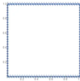
To use a conventional RBF (Kansa, 1990a; Kansa, 1990b; Kansa, 1992), the system described in
Eq. (11) is represented by randomly distributed nodes Nd and Nb, respectively, on the domain and
on the boundary Γ as shown in Fig. 4. This forms a set of N points ( ). In this study,
the rest of the formulations are given in the light of the use of single-domain or domain-decomposition approaches.
Figure 4: Domain and boundary nodal distribution in RBF.
4.1.1 Single-Domain RBF
For a conventional formulation and assuming a suitable RBF centered at a given number of points, the solution to Eq. (11) can be approximated using the direct collocation method as
Where is the radial basis function centered at and is the Euclidean norm. The
unknown coefficients
'
s
are determined by solving the system of N linear equations in Eq. (13)formed by applying the operators and to the approximation given by Eq. (12) at N selected
points; is applied to Nd nodes, is applied to boundary nodes on
1 and to the crack boundarynodes on
2. Throughout this work, use is made of the multiquadric RBF, √ where ris defined earlier as the radial distance defined between two points and c is a shape parameter that
needs to be calibrated to fine-tune the solution accuracy.
(13)
4.1.2 Domain-Decomposition Using RBF
Some geometrical crack configurations calls for the need of using the domain-decomposition
tech-nique. In this work, the domain-decomposition formulation assumes the original domain Ω to be
sub-divided into two sub-domains Ω1 and Ω2 with assumed solutions and , respectively.
The procedure described in Sect. 4.1.1 is then extended to handle such decomposed domains. This
requires the additional conditions, and , to be satisfied in order to
en-sure compatibility or continuity at the common boundary between the two subdomains. Conse-quently, the system of equations given by Eq. (13) for the single-domain RBF formulation is modi-fied to yield Eq. (14) for the domain-decomposition approach.
,
,
,
,
(14)
4.2 BEM and its Application for Mode III Crack Analysis
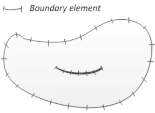
Figure 5: Discretization in BEM.
4.2.1 Single-Domain BEM
Applying the concept of weighted residual technique to Eq. (11a), noting that the operator ≡ ,
and integrating by parts twice, results in Eq. (15).
̅, ̅ Ω ∗ ̅, ̅ Γ ∗ ̅, ̅ Γ (15)
The weighting function, w*, in Eq. (15) is selected to be the fundamental solution which yields
the domain integral equations given by Eq. (16).
̅ ̅ ∗ ̅, ̅ Γ ̅ ∗ ̅, ̅ Γ (16)
Where
; ∗ ∗; ⋯ ⋯ ⋯ ; ∗
̅, ̅ (17)
Dividing the boundary into constant-type elements with w and q evaluated at mid-points
( , ) over each boundary element, the boundary integral equations are obtained by taking xi to
the boundary. This results in the boundary integral equations given by Eq. (18).
̅ ∗ ̅ , ̅ Γ ∗ ̅ , ̅ Γ (18)
For constant-element type, and are nodal values at mid-points, ̅ , of the ith element,
and ̅ are the coordinates of any point within the jth boundary element. Applying Eq. (18) at
̅ , , ⋯ , on both the crack and other boundaries, the boundary element equations are
obtained as given by Eq. (19).
(19)
∗ ̅ , ̅ Γ; ∗ ̅ , ̅ Γ; , , , ⋯ ,
The singular elements ( and ) can be computed using Eq. (20).
; (20)
Where Lj is the length of the jth element.
Once the system of algebraic equations given by Eq. (19) are solved for the boundary nodal
val-ues and , the solution at any domain point ̅ and its derivatives can be obtained by Eq. (21)
and Eq. (22), respectively.
̅ ∗ ̅ , ̅ Γ ∗ ̅ , ̅ Γ (21)
̅ ∗ ̅ , ̅ Γ ∗ ̅ , ̅ Γ (22)
4.2.2 Domain-Decomposition Using BEM
The crack problem can also be handled using the BEM domain-decomposition technique where each
subdomain is treated separately by applying the BEM in turn. Compatibility of the unknowns (w
and q) is enforced at the interface between the two sub-domains. The resulting set of equations are
solved to obtain the unknowns on the boundaries, as well as on the interface between them. Let,
nb1 = the number of boundary elements (hence, nodes) on Ω1
nb2 = the number of boundary elements (hence, nodes) on Ω2
ni = the number of interface elements (hence, nodes) along the interface between the two
subdo-mains.
This implies that the total number of unknowns in the system = nb1+nb2+2ni (since both the
heads and the fluxes are unknowns along the interface elements). To get the required number of equations needed to solve for the unknowns, the BEM equations given by Eq. (19) are applied on
the boundaries of each of the subdomains (Eq. (23)), in turn, resulting into nb1+nb2 equations. In
order to obtain the remaining 2ni equations, compatibility conditions, given by Eq. 24, are satisfied
at the interface.
, , ; , , (23a)
, , ; , , (23b)
; (24)
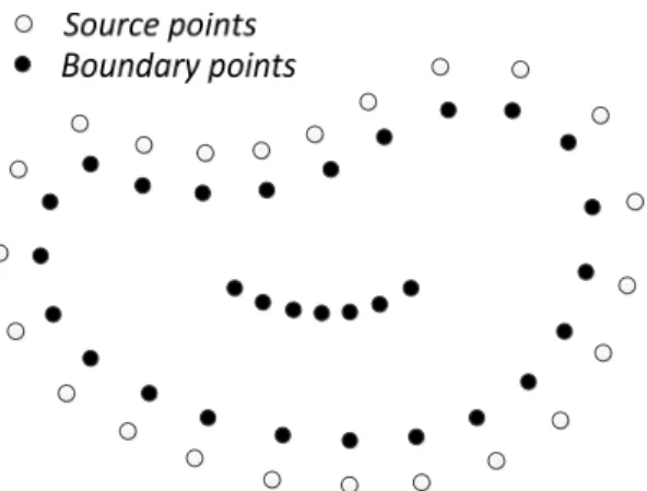
4.3 MFS and its Application for Mode III Crack Analysis
The MFS combines some interesting features and advantages of both the RBF and BEM. First, similar to the BEM, its use eliminates the need for domain discretization; only the boundary of the
problem needs to be discretized. Hence, it also requires the use of the fundamental solution w*
which satisfies the governing equation everywhere in the domain, except at the boundary. Second, the integration needed in BEM is avoided and, instead of using elements on the boundary as re-quired in the BEM, some distributed boundary nodes similar to the RBF are used. Again, as in the RBF, the MFS solution is approximated as a linear combination of the fundamental solution
cen-tered at some source points. But, due to the singularity behavior of w* at the source points, the
MFS does not make use of the boundary points as the source points. Instead, a set of points on a virtual boundary as shown in Fig. 6 are used. These virtual points serve as the centers of the
indi-vidual basis functions, the fundamental solutions,used in the approximation.
Figure 6: Source and boundary nodal distribution in MFS.
4.3.1 Single-Domain MFS
With w* centered at a given number of source points, the solution to Eq. (11) is approximated as
follows.
∗ (25)
Where are coefficients to be determined and are the off-boundary points (the source
points) located at a distance d normal to the original boundary. The coefficients can be
deter-mined by satisfying the boundary conditions at boundary points on the crack
2 and the rest ofthe boundary
1 as given by Eq. (26).∗
4.3.2 Domain-Decomposition Using MFS
The procedure for MFS based on the domain-decomposition technique is similar to that applied to
the RBF-based domain-decomposition in Sect. 4.1.2 by subdividing the original domain Ω into two
sub-domains Ω1 and Ω2, compatibility condition (functions of the assumed solution in Eq. (25)) is
enforced at the interface common to the two sub-domains thus and .
Therefore, the system of equations given by Eq. (26) is modified to yield the form given in Eq. (27).
∗
∗
∗
∗
∗
∗
∗
∗
(27)
5 PRELIMINARY PERFORMANCE CHECK AND SUGGESTED ENRICHMENTS
Some preliminary simulation runs for mode III loaded cracks were performed to verify the applica-bility and performance of the aforementioned formulations. As will be seen in the results section (Sect. 7), the outcome indicates that while BEM is successful in capturing the near-field solution behavior, the same cannot be said in the case of RBF and MFS. Due to this unsatisfactory behavior of the two latter methods at the crack-tip field, the present work utilizes the singular analytical solution of Eq. (9) to enrich them. This choice is made due to the fact that Eq. (9) captures the
near-field singularity behavior. Representing the nth enrichment term as the basis function given by
Eq. (28), the RBF and MFS formulations given in Sect. 4 are modified to yield enriched RBF and MFS referred to, here, as e-RBF and e-MFS respectively.
(28)
Another factor considered in the preliminary performance check is the need or otherwise of the use of domain-decomposition approach for each of the three methods. Again, it was found that the BEM works fine using the single-domain approach. This was made possible by defining the two
crack faces separated at a very small distance of units (approximately zero). On the other
hand, it was noticed that the use of domain-decomposition for both the RBF/e-RBF and MFS/e-MFS was necessary in order to yield satisfactory results.
5.1 e-RBF Formulation
Due to the inefficiency of Eqs. (13) and (14) to capture the singularity at the crack tip, an enrich-ment is proposed to the assumed approximate solution. Hence, Eq. (29) is proposed as a modified
form of Eq. (12), which involves addition of Ns singular terms as functions of the analytical solution
tip , and the system of algebraic equations given by Eq. (30) for the single-domain approach is
ultimately generated via the collocation procedure and taking (i.e. addition of one singular
term). This makes it possible to solve for the unknowns and .
‖ ‖ (29)
(30)
The e-RBF formulation based on domain-decomposition can be written in the form given by Eq. (31).
, ,
, ,
, ,
, ,
(31)
5.2 e-MFS Formulation
Similar to the case with RBF, Eqs. (26) and (27) for the MFS formulation cannot capture the sin-gularity at the crack tip, and enrichment given in Eq. (32) is proposed to the assumed approximate
solution. It also involves addition of Ns singular terms as functions of the analytical solution (cf.
Alves and Leitão, 2006) centered at the crack tip . Taking (i.e. addition of one singular
term), and collocating over the boundary points generates the system of algebraic equations given by Eq. (33), for the single-domain approach, which is solved for the unknowns and .
∗ ‖ ‖ (32)
∗
∗ (33)
, ∗ ,
, ∗
,
, ∗
∗
∗
,
, ∗
,
∗
∗
(34)
6 COMPUTATION OF SIF
Results of the crack-tip stress analysis using the BEM formulation reported in this work are ob-tained by, first, computing the J-integral of the problem and, subsequently, using it to evaluate the SIF. However, the e-RBF and e-MFS have an advantage of allowing the SIF to be obtained auto-matically as part of the solution. In all the analysis carried out in the present work, the enrichments
in these equations are limited to addition of one singular term each and, hence, . This choice
is valid due to the fact that the singular stresses manifest only in the first terms of the expansions
in Eq. (10). As a result, the last term in each of the expansions of w in Eqs. (29) and (32),
respec-tively, for the e-RBF and e-MFS formulations is √ . Comparing these enriched equations
in the vicinity of the crack tip ( → ) with Eq. (7), it can be deduced that ⁄ . This
allows automatic solution of the SIF as one of the unknown constants solved for in the e-RBF and e-MFS.
7 NUMERICAL RESULTS
Analysis of mode III cracks is performed to study the applicability and performance of the three mesh-reduction methods presented in this work. Depending on the method, position of the crack may call for the use of single-domain or domain-decomposition approaches. In all cases, unit plate width is used and the SIF is non-dimensionalized with respect to (See Sect. 3).
The results are generated after a series of parametric analysis for different configurations having different dimensions. Hence, for the sake of brevity, information about the number of elements (hence the number of degrees of freedom) used for the discretization of each of the mesh-reduction methods is reported in terms of the grid spacing. This makes it possible, if interested, for one to arrive at the number of elements used for all the methods for any given dimensions. Free triangular element type is used with a maximum size of 0.005 fixed for all the cases solved using the FEM.
However, a typical example about the the number of elements for a case with a/ . is reported
in each of the cracked geometry presented.
7.1 Plate with Central Crack
The rectangular plate shown in Fig. 7(a) is analyzed using the BEM and the two enriched methods (e-MFS and e-RBF). This case can represent either an internal central crack in a plate of
fig-ure). Due to the symmetry of the problem, it doesn’t necessitate the use of domain-decomposition technique. Hence, half or quarter of the plate is modeled as shown in Fig. 7(b) which corresponds to the case of central edge crack or central internal crack, respectively. Typical discretizations for the three mesh-reduction methods applied to this problem are shown in Fig. 8.
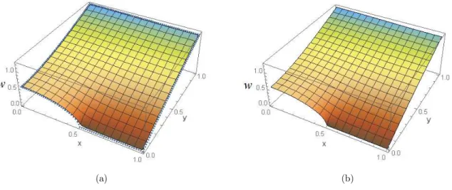
Figs. 9 to 11 show typical predictions by the RBF/e-RBF, BEM and MFS/e-MFS. Evidence is shown on the failure of conventional RBF and MFS to model the crack-tip field satisfactory (Figs. 9(a) and 11(a)). This issue is resolved with the use of e-RBF and e-MFS as seen in Figs. 9(b) and 11(b). However, as shown in Fig. 10, the standard BEM has interestingly modeled the crack-tip field without the necessity of enrichment. Both RBF/e-RBF and MFS/e-MFS provide closed-form solution, each, of the displacement which is valid for both the domain and boundary of the prob-lem. On the other hand, as the name implies, the boundary element method (BEM) provides a boundary solution at discrete nodes (shown as dots in Fig. 10(a)) at the center of the constant-type boundary elements which are used to obtain the closed-form solution of the displacement (See Eq. (21)) that is valid within the domain (shown as a surface in Fig. 10(a)). Although not required, but the two sets of the BEM results (boundary and domain) are interpolated to yield the overall solution which enables clearer view shown in Fig. 10(b) of the successful prediction of the crack-tip field solution by the BEM.
SIF results achieved for different crack sizes for a modeled domain of unit square are reported in Table 1 along with other literature results to demonstrate the reliability of the presented methods. Acceptable results are obtained using regular e-RBF and e-MFS grid distributions, where a
mini-mum grid spacing of / is adopted for both the two methods. The off-set distance of .
for the source points in the e-MFS is used, while choosing the shape parameter c in the
multiquad-ric RBF within . . is found to be satisfactory. The BEM discretization consists of a
minimum grid spacing of / 0 and / 0 on the crack-containing edge and the rest of the edges,
respectively. For a typical case with / . , the mentioned grid specifications result in 3,841,
241 and 1,201 degrees of freedom for the e-RBF, e-MFS and BEM, respectively, compared to 4,629 degrees of freedom used in FEM for the same case.
(a) (b)
(a) Discretization using RBF/e-RBF (b) Discretization using standard BEM
(c) Discretization using MFS/e-MFS
Figure 8: Half model of a square plate with central edge crack.
(a) (b)
(a) (b)
Figure 10: Typical result for a cracked plate: domain of unit squaremodeled using standard BEM showing (a) boundary (dots) and domain (surface) solutions (b) Overall solution.
/
. . . .
Present
e-RBF 1.0028 1.0166 1.0401 1.0757 1.1278 1.2087 1.3362 1.5696 2.1246
BEM 1.0026 1.0167 1.0404 1.0767 1.1299 1.2099 1.3368 1.5646 2.1101
e-MFS 1.0035 1.0176 1.0411 1.0771 1.1305 1.2105 1.3376 1.5660 2.1131
Liao et al. (2015) 1.0043 1.0176 1.0411 1.0771 1.1305 1.2105 1.3376 1.5660 2.1137
Sun et al. (2003) 1.001 1.016 1.040 1.077 1.132 1.213 1.346 - -
Yuanhan (1992) 1.0004 1.0170 1.0410 1.0771 1.1305 1.2105 1.3377 1.5648 2.0679
Murakami (1987) 1.0041 1.0170 1.0398 1.0753 1.1284 1.2085 1.3360 1.5650 2.1133
Table 1: SIF results for plate with central crack.
(a) (b)
7.2 Off-Central Crack
Since in real life cracks are not always central, another configuration of mode III crack problem is considered, the off-central crack shown in Fig. 12. It can be noticed, from the figure, that the prob-lem doesn’t warrant the use of symmetry line passing through the crack. Hence, its solution require more efforts than the previous crack configuration solved. Two possibilities of solution strategy exist in such a situation namely, modeling the full domain shown in Fig. 12(a) with the boundary condi-tions shown in Fig. 12(b) or the use of domain-decomposition which results in subdividing the prob-lem into a number of subdomains (two in this case) dictated by the number of cracks as shown in Fig. 12(c). It is unarguably clear that the first strategy is simpler and less computationally expen-sive due to lesser number of unknowns and, hence, number of equations needed to be solved. Pre-liminary simulation runs are conducted to study the feasibility of the first strategy. It is found that of the three mesh-reduction methods in this work, only the BEM is able to satisfactorily model such problem using the full-model approach: Both the e-RBF and e-MFS fail to achieve reasonable solu-tions. Consequently, use of domain-decomposition is made in the two latter methods. Typical dis-cretization schemes for the three methods used in solving the off-central cracks are shown in Fig. 13 where it is clear that both e-RBF and e-MFS are discretized in such a way suitable for domain-decomposition while the BEM is discretized to tackle the problem as a single domain.
Table 2 shows the SIF results achieved for different cases of the off-central crack. It can be seen that although the BEM results are obtained using the full/single-domain model, yet the results compare favorably with the e-RBF and e-MFS domain-decomposition approaches. The same prob-lems are modeled using FEM and the results are also presented in the table to serve as a means for verifying the predictions of the three mesh-reduction methods presented. In this case, maintaining the minimum grid spacing of 1/60 for the e-RBF still works but with a shape parameter c=0.15. However, the minimum grid spacing in the case of e-MFS is reduced to 1/100 and the off-set tance of 0.1 for the source points is used. Minimum grid spacing of 1/300 is used for the BEM
dis-cretization of this problem. The FEM solution for a typical case with : : and : :
: : is obtained using a total of 5,922 elements compared to 3,961, 391 and 1,501 degrees of
free-dom used in e-RBF, e-MFS and BEM, respectively, for the same case.
(a) (b) (c)
(a) (b) (c)
Figure 13: Typical geometry with crack that is not aligned with any line of symmetry discretized using (a) e-RBF (b) standard BEM, and (c) e-MFS.
: :
:
∶ . ∶ ∶
e-RBF BEM e-MFS FEM e-RBF BEM e-MFS FEM e-RBF BEM e-MFS FEM
: : 1.4203 1.4203 1.4133 1.4192 1.2705 1.2673 1.2671 1.2662 1.1488 1.1504 1.1487 1.1496
: : 1.3403 1.3402 1.3363 1.3392 1.1912 1.1877 1.1881 1.1869 1.0991 1.0923 1.0903 1.0916
: : 1.2855 1.2913 1.2863 1.2906 1.1356 1.1343 1.1344 1.1336 1.0534 1.0544 1.0526 1.0537
: : 1.5474 1.5501 1.5507 1.5477 1.3849 1.3868 1.3850 1.3849 1.2446 1.2406 1.2374 1.2392
: . : 1.3829 1.3819 1.3788 1.3809 1.2340 1.2297 1.2300 1.2289 1.1212 1.1231 1.1209 1.1222
: : 1.2887 1.2943 1.2893 1.2936 1.1372 1.1377 1.1388 1.1371 1.0497 1.0568 1.0549 1.0562
: : 1.9057 1.9225 1.9343 1.9237 1.6949 1.7127 1.6543 1.7012 1.4869 1.4916 1.4896 1.4923
: : 1.4673 1.4688 1.4674 1.4674 1.3133 1.3124 1.3112 1.3112 1.1937 1.1847 1.1831 1.1837
: : 1.2954 1.2996 1.2947 1.2988 1.1486 1.1437 1.1445 1.1431 1.0551 1.0610 1.0591 1.0604
Table 2: SIF results for plate with off-central crack.
7.3 Two Parallel Cracks
As shown in Fig. 14, plate containing two parallel cracks is considered as another case of the mode
III crack problem. Separated by a distance , these cracks can represent the case of either two
internal cracks in a plate of dimensions (as shown in the figure) or the case of two edge
cracks on a plate with dimensions . In either case, similar to the case of off-central crack
of the cracks since the configuration doesn’t result in the symmetry line (shown in dashed) to pass through the crack lines. Consequently, even if half or quarter of the plate is modeled which corrsponds to the case of two edge cracks or two internal cracks, respectively, the use of RBF and e-MFS domain-decomposition as shown in Fig. 12(c) is necessary. However, as in the case of the off-central crack, the BEM is capable of handling the problem without domain-decomposition (See Fig. 13(b)).
Results obtained for several cases of the problem based on the three formulated methods are shown in Table 3 along with the predictions by FEM for verification. The off-set distance in the e-MFS for this problem is 0.13 while the shape parameter in the e-RBF is 0.15. Minimum grid
spac-ings of / , / and / are used for the e-RBF, BEM and e-MFS, respectively. Based on
the mentioned grid specifications, the degrees of freedom used for a typical case with : :
and : : : : are 3,961, 1,261 and 551 for the e-RBF, e-MFS and BEM, respectively. The
FEM discretization for the same geometry is achieved using 5,959 elements.
(a) (b)
Figure 14: Plate with two parallel cracks: (a) Full model (b) Quarter model due to symmetry.
: :
:
∶ . ∶ ∶
e-RBF BEM e-MFS FEM e-RBF BEM e-MFS FEM e-RBF BEM e-MFS FEM
: : 1.3287 1.3305 1.3269 1.3296 1.1774 1.1782 1.1764 1.1776 1.0823 1.0848 1.0764 1.0843
: . : 1.2471 1.2494 1.2443 1.2489 1.0928 1.0935 1.0914 1.0931 1.0176 1.0197 1.0108 1.0195
: : 1.1981 1.2006 1.1933 1.2003 1.0366 1.0371 1.0336 1.0368 0.9753 0.9764 0.9661 0.9762
: : 1.4970 1.4976 1.4971 1.4961 1.3353 1.3361 1.3349 1.3351 1.2049 1.2072 1.2017 1.2066
: . : 1.3248 1.3267 1.3230 1.3262 1.1712 1.1721 1.1703 1.1718 1.0796 1.0822 1.0742 1.0819
: : 1.2362 1.2384 1.2319 1.2381 1.0755 1.0759 1.0727 1.0757 1.0084 1.0097 1.0010 1.0095
: : 1.8980 1.8939 1.9031 1.8867 1.6872 1.6873 1.6867 1.6867 1.4798 1.4768 1.4822 1.4751
: . : 1.4346 1.4359 1.4343 1.4349 1.2781 1.2791 1.2778 1.2785 1.1599 1.1631 1.1564 1.1625
: : 1.2633 1.2655 1.2596 1.2652 1.1048 1.1054 1.1025 1.1052 1.0314 1,0330 1.0237 1.0327
7.4 Relative Performance of the Three Mesh-Reduction Methods
Relative applicability and performance of the three mesh-reduction methods in the present study can be assessed based on the foregoing discussion. Summary of the same is given in Table 4 in terms of need, or otherwise, of the following: (i) enrichment, (ii) domain-decomposition, (iii) auto-matic evaluation of SIF alongside the solution, (iv) parameter calibration, (v) availability of funda-mental solution, and (vi) integration.
BEM MFS RBF
Standard e-MFS Standard e-RBF
Integration required Yes No No No No
Fundamental solution required Yes Yes Yes No No
Need for domain discretization No No No Yes Yes
Need for parameter calibration No Yes Yes Yes Yes
Captures crack-tip singularity Yes No Yes No Yes
Enrichment status No No Yes No Yes
Modeled with symmetry Crack-tip field solution
Far-field solution
Modeled without symmetry Single-domain Crack-tip field solution Far-field solution
Domain-decomposition Crack-tip field solution
Far-field solution
Provides accurate solution Fails to provide accurate solution
Table 4: Summary of performance of the three mesh-reduction methods in the benchmarked mode III problems.
8 CONCLUSIONS
Acknowledgement
The author would like to acknowledge the support provided by the Deanship of Scientific Research at King Fahd University of Petroleum & Minerals (KFUPM) under Research Grant JF-151003.
References
Alves, C.J.S., Leitão, V.M.A. (2006). Crack analysis using an enriched MFS domain decomposition technique. Engi-neering Analysis with Boundary Elements 30: 160-166.
Ang, W.T. (1999). A complex variable boundary element method for antiplane stress analysis around a crack in some nonhomogeneous bodies. Journal of the Chinese Institute of Engineers 22: 753-761.
Bernal, F., Gutierrez, G., Kindelan, M. (2009). Use of singularity capturing functions in the solution of problems with discontinuous boundary conditions. Engineering Analysis with Boundary Elements33: 200-208.
Bernal, F., Kindelan, M. (2009). On the enriched RBF method for singular potential problems. Engineering Analysis with Boundary Elements 33: 1062-1073.
Blandford, G.E., Ingraffea, A.R., Liggett, J.A. (1981). Two-dimensional stress intensity factor computations using the boundary element method. International Journal for Numerical Methods in Engineering 17: 387-404.
Brebbia, C.A., Dominguez, J. (1989). Boundary Elements: An Introductory Course. Computational Mechanics Pub-lications (Southampton).
Chen, J.T., Chen, K.H., Yeih, W., Shieh, N.C. (1998). Dual boundary element analysis for cracked bars under tor-sion. Engineering Computations 15: 732-749.
Chen, J.T., Chen, Y.W. (2000). Dual boundary element analysis using complex variables for potential problems with or without a degenerate boundary. Engineering Analysis with Boundary Elements 24: 671-684.
Chen, Y.Z., Lin, X.Y. (2007). Singular integral equation method for multiple Zener–Stroh crack problems in anti-plane elasticity. Engineering Analysis with Boundary Elements31: 22-27.
Chiang, C.R. (1987). Slightly curved cracks in anti-plane strain. International Journal of Fracture32: 63-66. Dolbow, J., Möes, N., Belythscko, T. (2000). Modeling fracture in Mindlin-Reissner plates with extended finite ele-ment method, International Journal of Solids and Structures 37: 7161-7183.
Gu, Y.T., Wang, W., Zhang, L.C., Feng, Z.Q. (2011). An enriched radial point interpolation method (E-RPIM) for analysis of crack tip fields. Engineering Fracture Mechanics 78: 175-190.
Irwin, G.R. (1958). Fracture. Handbuch der Physik, Springer, Berlin: 551-590.
Johnston R.L., Fairweather, G., Karageorghis, A. (1987). An adaptive indirect boundary element method with appli-cations. In: Tanaka, M., Brebbia, C.A., editors. Boundary elements VIII, proceedings of the eighth international conference. New York, Springer: 587–98.
Kansa, E.J. (1990a). Multiquadrics–A scattered data approximation scheme with applications to computational fluid-dynamics–I surface approximations and partial derivative estimates. Computers & Mathematics with Applications 19: 127–145.
Kansa, E.J. (1990b). Multiquadrics–A scattered data approximation scheme with applications to computational fluid-dynamics–II solutions to parabolic, hyperbolic and elliptic partial differential equations. Computers & Mathe-matics with Applications19: 147–161.
Kansa, E.J., Carlson, R.E. (1992). Improved accuracy of multiquadric interpolation using variable shape parameters. Computers & Mathematics with Applications 24: 99–120.
Kermanidis, Th. B., Mavrothanasis, F.I. (1995). Calculation of mode III stress intensity factor by BEM for cracked axisymmetric bodies. Computational Mechanics 16: 124-131.
Krysl, P., Belytshcko, T. (1999). The Element Free Galerkin Method for Dynamic propagation of arbitrary 3-D cracks, International Journal for Numerical Methods in Engineering 44: 767–800.
Kupradze, V.D., Aleksidze, M.A. (1964). The method of functional equations for an approximate solution of certain boundary value problems. USSR Computational Mathematics and Mathematical Physics 4: 82–126.
Leung, A.Y.T., Tsang, K.L. (2000). Mode III two-dimensional crack problem by two-level finite element method. International Journal of Fracture102: 245–258.
Liao, M., Tang, A., Hu, Y-G. (2015). Calculation of mode III stress intensity factors by the weak-form quadrature element method. Archive of Applied Mechanics 85: 1595-1605.
Liu, N., Altiero, N.J. (1992). An integral equation method applied to mode III crack problems. Engineering Fracture Mechanics 41: 587-596.
Ma, S.W. (1988). A central crack in a rectangular sheet where its boundary is subjected to an arbitrary anti-plane load. Engineering Fracture Mechanics 30: 435-443.
Ma, S.W. (1989). A central crack of mode iii in a rectangular sheet with fixed edges. International Journal of Frac-ture39: 323-329.
Ma, S.W., Zhang, L.X. (1991). A new solution of an eccentric crack off the center line of a rectangular sheet for mode-III. Engineering Fracture Mechanics 40: 1-7.
Martínez, J., Domínguez, J. (1984). On the use of quarter-point boundary elements for stress intensity factor compu-tations. International Journal for Numerical Methods in Engineering20: 1941-1950.
Mews, H., Kuhn, G. (1988). An effective numerical stress intensity factor calculation with no crack discretization. International Journal of Fracture38: 61-76.
Murakami, Y. (1987). Stress Intensity Factors Handbook. 1st ed. Pergamon Press, Oxford (Oxfordshire).
Paulino, G.H., Saif, M.T.A., Mukherjee, S. (1993). A finite elastic body with a curved crack loaded in anti-plane shear. International Journal of Solids and Structures 30: 1015-1037.
Poullikkas, A., Karageorghis, A., Georgiou, G. (1998). Methods of fundamental solutions for harmonic and bi-harmonic boundary value problems. Computational Mechanics 21: 416-423.
Sáez, A., Gallego, R., Dominguez, J. (1995). Hypersingular quarter-point boundary elements for crack problems. International Journal for Numerical Methods in Engineering 38: 1681-1701.
Sih, G.C. (1965). Stress distribution near internal crack tips for longitudinal shear problems. Journal of Applied Mechanics32: 51-58.
Sih, G.C. (1966). On the Westergaard method of crack analysis. International Journal of Fracture Mechanics 2: 628– 631.
Snyder, M.D. (1973). Crack tip stress-intensity factors in finite anisotropic plates. Technical Report AFML-TR-73-209, Air Force Materials Laboratory (Ohio).
Sun, Y-Z., Yang, S-S., Wang, Y-B. (2003). A new formulation of boundary element method for cracked anisotropic bodies under anti-plane shear. Computer Methods in Applied Mechanics and Engineering 192: 2633-2648.
Ting, K., Chang, C-S., Chang, K-K. (1994). Alternating method applied to analyse mode-III fracture problems with multiple cracks in an infinite domain. Nuclear Engineering and Design 152: 135-145.
Ting, K., Chang, K-K., Yang, M.F. (1995). Analysis of mode-III fracture problem with multiple cracks by boundary element alternating method. International Journal of Pressure Vessels and Piping 62: 259-267.
Vroonhoven, J.C.W. (1995). Stress intensity factors for curvilinear cracks loaded under anti-plane strain (Mode III) conditions. International Journal of Fracture70: 1-18.
Wang, L., Chen, J-S., Hu, H-Y. (2010). Subdomain radial basis collocation method for fracture mechanics. Interna-tional Journal for Numerical Methods in Engineering83: 851-876.
Wang, Y.H., Cheung, Y.K., Woo, C.W. (1992). Anti-plane shear problem for an edge crack in a finite orthotropic plate. Engineering Fracture Mechanics 42: 971-976.
Westergaard, H.M. (1939). Bearing pressures and cracks. Journal of Applied Mechanics 6: 49–53.
Williams, M.L. (1952). Stress singularities resulting from various boundary conditions in angular corners of plates in extension. Journal of Applied Mechanics 19: 526–528.
Williams, M.L. (1957). On the stress distribution at the base of a stationary crack. Journal of Applied Mechanics 24: 109–114.
Wu, W-L. (2009). Dual boundary element method applied to antiplane crack problems. Mathematical Problems in Engineering: 1-10.
Xanthis, L.S., Bernal, M.J.M., Atkinson, C. “The treatment of singularities in the calculation of stress intensity fac-tors using the boundary integral equation method". Computer Methods in Applied Mechanics and Engineering 26 (1981): 285-304.
Yuanhan, W. (1992). Analysis of an edge-cracked body subjected to a longitudinal shear force. Engineering Fracture Mechanics 42: 45-50.
Yuanhan, W. (1993). SIF calculation of an internal crack problem under anti-plane shear. Computers & Structures 48: 291-295.
Zhang, X.S. (1987). The general solution of a central crack off the center line of a rectangular sheet for mode III. Engineering Fracture Mechanics 28: 147-155.
Zhang, X.S. (1988). The general solution of an edge crack off the center line of a rectangular sheet for mode III. Engineering Fracture Mechanics 31: 847-855.