W. Huacasi
Laboratory of Mathematics, State University of Norte Fluminense 28015 620 Campos dos Goytacazes, RJ. Brazil
W. J. Mansur and J. P. S.
Azevedo
Civil Engineering Department, COPPE Federal University of Rio de Janeiro 21945 970 Rio de Janeiro, RJ. Brazil [email protected] and [email protected]
A Novel Hypersingular B.E.M.
Formulation for Three-Dimensional
Potential Problems
In this paper a direct boundary element hypersingular formulation for three-dimensional potential problems is presented. It is shown that the integrals which arise in this formulation are Cauchy principal value integrals, i.e., divergent terms of the finite part integrals cancel one another. Since in the present formulation the collocation points are placed within boundary elements, free terms are computed by simple expressions. The resulting integrals are one-dimensional and regular, therefore can be evaluated by Gaussian quadrature. For the numerical implementation, both linear and quadratic isoparametric triangular and quadrangular elements were used. Numerical results are presented to show the efficacy of the proposed hypersingular formulation.
Keywords: Boundary element method, hypersingular formulation, cauchy principal value, finite part integral
Introduction
Hypersingular integrals play an important role in the recent development of boundary element methods (BEM). Many hypersingular integral formulations have been proposed and applied to solve boundary value problems using boundary element techniques. One can distinguish two main approaches: those which use the Cauchy Principal Value (CPV) and those which use formulations in terms of the Finite Part (FP) (see Guiggiani, 1995; Mantic, 1994; Sladek and Sladek, 1996; Tanaka, Sladek and Sladek, 1994). One of the hypersingular formulations in terms of Cauchy principal values has been developed by Mansur, Fleury and Azevedo (1997) for two-dimensional potential problems. This approach ensures that the singular terms cancel out. The hypersingular equation is obtained by assuming that the solution is Hölder continuous ruling out collocation points on edges and corners, so that discontinuous elements have been adopted. The finite part approach was used, for instance, in papers by Guiggiani (1995) and Mantic (1994) and required the evaluation of additional free terms. An alternative approach that results very simple expressions to calculate the hypersingular integral was proposed by Kolm and Rokhlin (2001), however this method is restricted to two-dimensional problems only. 1
This paper presents a hypersingular formulation for three-dimensional potential problems using Cauchy principal value integrals. These CPV integrals are computed by using Hadamard's FP, following the one-dimensional technique developed by Brandão (1987). The existence of Cauchy's principal value integrals is explained. Collocation points are placed inside the boundary elements so that free terms can be computed through simple expressions. The resulting integrals are one-dimensional and regular and can be evaluated by Gaussian quadrature. In the numerical implementation, triangular and quadrangular linear or quadratic boundary elements have been used. We compare results of numerical implementation of our formulation and BEM formulation based on the Classical Boundary Integral Equation (we call it “classical formulation”).
Nomenclature
) (x
n = exterior normal to the boundary )
(x
pn = normal derivative of the potential function )
, (xξ
p∗ = normal derivative of the fundamental solution )
(x
u = potential function )
, (xξ
u∗ = fundamental solution
x
= point of the boundary) (ξ
ε
B = small ball of radius ε centered at the point ξ i
C = coefficient of the Laurent series, i=0,1,2,... E = number of the boundary elements
e
M = number of geometrical nodes of element Γe N = total number of functional nodes
g
N = number of Gauss point
Greek Symbols
x
ν = unit vector
ξ = source point (functional node)
i
τ
= orthogonal direction, i=1,2 ), (η1η2
φf = interpolation functions )
, (η1η2
ψm = shape functions
e
Γ = boundary element
σ
Γ = boundary element where the source point is located
Hypersingular Boundary Integral Equation
The solution of the boundary value problem for Laplace’s equation ∇2u=0 in Ω⊂IR3 is considered here. The numerical solution of this problem can be obtained by using the Classical Boundary Integral Equation (CBIE), see Brebbia, Telles and Wrobel (1984):
x n x
n xu xd u x p xd
p u
c +
∫
Γ =∫
ΓΓ ∗ Γ
∗( , ) ( ) ( , ) ( )
) ( )
Here x∈Γ, Γ is the boundary of Ω, ξ∈IR3\Γ is the source point,
Γ ∪ Ω ∈
Ω ∈ =
), ( \ if
0
, if 1 )
( 3
IR c
ξ ξ ξ
u(x) is the potential or density function, n(x) is the exterior normal to the boundary and pn(x)=∇u⋅n(x) is the normal derivative. The fundamental solution u∗of Eq. (1) and its normal derivativep∗ are given by
( )
r xu 1
4 1 ,
π ξ =
∗ ,
( )
1 ( ( ))4 1 ,
2 n x
r x
pn∗ =− νx⋅
π
ξ ,
wherer = | x -ξ | andνx=∇xr=
(
∂r∂x1,∂r∂x2,∂r∂x3)
is a unit vector.The hypersingular formulation arises by taking the directional derivative of Eq. (1), with respect to the source point ξ. Note that in three-dimensional integral equations, strong singularities and hypersingularities exist whenever the source pointξ is placed on the boundary.
When the source point is situated inside the domain Ω, functions )
, ( x
u∗ξ and p∗(ξ,x) are regular. Thus, Eq. (1) can be differentiated along any direction ω yielding the following boundary integral equation:
x n x
n xu xd u x p xd
p
p +
∫
Γ =∫
ΓΓ ∗ Γ
∗ ( , ) ( ) ( , ) ( )
)
(ξ ,ωξ ,ω ξ
ω . (2)
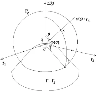
If the source pointξis located onΓ, Γ augmented by a small ball Bε(ξ) centered at ξ with radius ε (Fig. 1). The integrals are evaluated now along a new boundary consisting of two parts:Γ-Γε and Γε, being Γε the boundary of Bε(ξ), as shown in Fig. 1. The boundary integral equation obtained by this procedure is given by Eq. (3), where in order to restore the originalΩ domain andΓ boundary, one takes the limit when ε → 0 in this equation:
Γ −
+ ∗
Γ − Γ
∗
→
∫
pn xu x u x pn x d xp ( ) lim [ , ( , ) ( ) , ( , ) ( )]
0 ξ ξ
ξ ω ω
ε ω
ε
0 )]
( ) , ( ) ( ) , (
[ , , =
Γ −
+ ∗
Γ ∗
∫
εε
ξ
ξ ω
ω n x
n xu x u x p x d
p , (3)
where
(
( ))
4 1 ) , (
2
, ν ωξ
π ξ
ω = ⋅
∗
x r x
u ,
(
)
3 ,
4
)) ( ) ( ( )) ( ( ) ( 3 ) , (
r
x n x
n x
pn x x
π
ξ ω ν
ξ ω ν ξ
ω =− ⋅ ⋅ − ⋅
∗ .
Figure 1. Domain augmented by a hemisphere of radius εε centered at ξξ.
The limit indicated in Eq. (3) exists in a neighborhood of ξ whenever u∈C1,α, 0≤α≤1, i.e.:
) | (| ) )( ( ) ( )
(x =uξ +u, ξ x −ξ +O x−ξ 1+α
u k k k ,
) | (| ) ( )
( ,
, x =u ξ +O x−ξ α
uk k , (4)
for k=1,2,3; ξ→x. The limit of the second integral in Eq. (3) can be considered by parts:
∫
Γ ∗
→ Γ
=
∗
ε
ε ω
ε p ξ xu xd
Ip lim n, ( , ) ( )
0
and
∫
Γ ∗
→ Γ
=
∗
ε
ε ω
ε u ξ x p xd
I n
u lim0 , ( , ) ( ) .
Taking into account that on boundary Γε:
(
)
(
)
⋅ −
=
⋅ =
=
∗ ∗
, ) ( ) ( 4
2
, ) ( ) ( 4
1 ), (
3 ,
2 ,
ξ ω ε
π
ξ ω ε
π ν
ω ω
x n p
x n u
x n
n x
and using Eq. (4) and considering that on Γε :
ε ξ ) ( )
( k k
k x x
n = − one obtains:
(
)
(
)(
)
Γ ⋅ ∇ ⋅ + Γ ⋅
−
=
∫
∫
Γ Γ
→
∗
ε ε
ε ε
ε ε ξ
ξ ω ξ
ε ξ ω
π u nx d
x n d u x n
Ip lim () () () () ( ) x() ()
2 1
2 3
(
)(
)
∫
Γ
→ ∇ ⋅ Γ
⋅ =
∗
ε
ε
ε ε ξ
ξ ω
π u nx d
x n
I x
u ( ) ( )
) ( ) ( lim 4 1 2 0 .
Therefore, Eq.(3) can be written as:
(
)
(
)(
)
Γ ⋅ ∇ ⋅ + Γ ⋅ −∫
∫
Γ Γ → ε ε ε ε ε ω ξ ε ξ ω π ξ ε ξ ω πξ nx u d nx u nxd
p () () x() ()
4 3 ) ( ) ( ) ( 2 1 lim ) ( 2 3 0 ,
∫
Γ − Γ ∗ ∗→ − Γ
=
ε
ξ
ξ ω
ω
εlim0 [u, ( ,x)pn(x) pn, ( ,x)u(x)]d x. (5)
The limit of the second integral on the l.h.s. of equation (5) is
equal to ( ), 2
1 ξ
ω
p as shown in Appendix A1. Therefore, for )
( )
(ξ ξ
ω =n :
(
)
∫
∫
ε Γ − Γ ∗ ∗ → ε ε Γ ε →ε ε ξ Γ = ξ − ξ Γ
ξ ⋅ π −
ξ ,n n n,n x
n u( )d lim [u(,x)p(x) p (,x)u(x)]d ) ( n ) x ( n lim ) ( p 0 3 02 1 2 1 (6)
If the potential field is constant in the augmented domain )
( ) (
, ξ
ε u x =u
Ω ∪
Ω and pn=0, thus in Eq. (6):
(
)
(
)
∫
∫
Γ − Γ → Γ → Γ ⋅ ⋅ − ⋅ = Γ ⋅ ε ε ξ π ν ξ ν ξ ν ξ ε ξπ ε ε
ε x
x x
x u d
r x n n n d u n x n ) ( 4 )) ( ( ) ( 3 )) ( ( lim ) ( ) ( ) ( 2 1 lim 3 0 3 0
Therefore, the equation for the normal derivative in ξ∈Γ, is obtained in the CPV form, (see Fig. 2):
, )]} ( ) ( )[ , ( ) ( ) , ( { ) ( 2 1 , ,
∫
Γ ∗∗ − − Γ
= n n nn x
n CPV u x p x p x ux u d
p ξ ξ ξ ξ (7)
where
(
( ))
4 1
2
, ν ξ
πr n
u∗n= x⋅ ,
(
)
3 , 4 )) ( ) ( ( )) ( ( ) ( 3 r x n n x n npnn x x
π ξ ν
ξ
ν ⋅ ⋅ − ⋅
− =
∗ .
Figure 2. Domain of CPV integrations.
The integral equation for boundary derivatives (when ξ∈Γ) in
∫
Γ
∗
∗ − − Γ
=CPV u x pn x pn x u x u d x p
i i
i( ) { ( , ) ( ) ( , )[ ( ) ( )]}
2 1
,
, ξ ξ ξ
ξ τ τ
τ , (8) where
(
( ))
4 1 2, ν τ ξ
π
τ x i
r u
i = ⋅
∗ ,
(
)
3 , 4 )) ( ) ( ( )) ( ( ) ( 3 r x n x npn x i x i
i π ξ τ ν ξ τ ν
τ =− ⋅ ⋅ − ⋅
∗ .
The integral equations (7) and (8), obtained here in CPV terms, can also be calculated, following Brandão (1987), as FP integrals, by using Taylor expansion and polar coordinates, as shown in the Section 3. In addition to the normal derivative, two tangent derivatives in two arbitrary orthogonal directionsτi (i=1,2) can be calculated in order to define completely the gradient at any boundary point.
Existence of the Cauchy's Principal Value
The Hölder continuity condition, Eq. (4), is necessary for the existence of CPV. If the integral with hypersingular kernel exists in the CPV sense, this integral exists as a sum of finite parts. The developments to be performed in what follows require two successive coordinates changes; the first from cartesian to natural coordinates and the second from natural to polar coordinates:
∫
∫
Γ Γ
∗ Φ = Γ
= θ ρ θ ρ θ ρ η η η η ξ , , 2 1 2 1
, ( ,x) ( , )|G|d d F( , )d
p
h nn , (9)
with ) 1 ( ) ( ) ( ) , ( 1 2
2 F O
F
F = + +
ρ θ ρ
θ θ
ρ , (10)
∫
∫
Γ Γ
∗ = Γ
= θ ρ θ ρ θ ρ η η ξ , , 2 1
, ( ,x)|G|d d f( , )d
p
s nn , (11)
with ) 1 ( ) ( ) ( ) , ( 1 2
2 f O
f
f = + +
ρ θ ρ
θ θ
ρ , (12)
∫
∫
Γ Γ
∗ Φ = Γ
= θ ρ θ ρ θ ρ η η η η ξ , , 2 1 2 1
, ( ,x) ( , )|G|d d g( , )d
u
g n , (13)
where ) 1 ( ) ( ) ,
( g1 O
g = +
ρ θ θ
ρ . (14)
Expressions (10), (12) and (14) can be used to calculate CPV in terms of finite parts. The existence of CPV in Eq. (7) and taking into account Eqs. (7), (9) and (11) yield:
0 )] ( ) ( [ | | ln lim 2 = −
and
0 )
( )] ( ) ( [ 1 lim
2 0
2 2
0 =
−
∫
→ βθ θ
θ θ ε π
ε d
f F
. (16)
The results above can be easily checked since F2=φ0ff2 and
∑
+ =f
f A T f
f
F 1
4 1 0
1 φ π13φ , see Appendix A3. Likewise, for Eq. (13), one has:
0 ) ( | | ln lim
2 0
1
0
∫
=→ ε θ θ
π
ε g d . (17)
This is due to the presence, in g1, of the inner products of orthogonal vectors, (see Section 4.1). Therefore, with (15), (16) and (17)
∫
Γ
∗
∗ − − Γ
= n n nn x
n CPV u x p x p x u x u d
p ( ) { ( , ) ( ) ( , )[ ( ) ( )]}
2 1
,
, ξ ξ ξ
ξ
holds, as well as
∫
Γ
∗
∗ − − Γ
x n
n n
n x p x p x u x u d
u
CPV { , (ξ, ) ( ) , (ξ, )[ ( ) (ξ)]}
x n
n n
n x p x p x u x u d
u − − Γ
∫
= ∗ ∗
Γ{ , (ξ, ) ( ) , (ξ, )[ ( ) (ξ)]} (18)
In formulations in which p∗ is not multiplied by [u(x)−u(ξ)] one must not to ignore free terms. In Eq. (6), for instance, the integral on the r.h.s. does not exist in the CPV sense but its finite part can be computed. The left hand side of Eq. (6) can be written as a Laurent series as
..., ...
)] ( ) , ( ) ( ) , ( [
lim 1 22
2 2 1 0 ,
,
0 − Γ = + + + + + +
− − Γ
− Γ
∗ ∗
→
∫
r Cr CrC r C C d x u x p x p x
un n nn x
ε
ξ ξ
ε
(19)
when
r
→
0
; the terms containing C1,C2,...vanish and one is left with C0 (the finite part) plus terms which tend to infinity with growing orders of singularity. Eq. (19) has no limit; thus(
)
∫
Γ
→ Γ
⋅ −
ε
ε
ε ε ξ
ξ π
ξ nx n u d
pn ( ) ( ) ( )
2 1 lim ) ( 2 1
3
0 (20)
has no limit either, but it has the same finite part and same singular terms coefficients C1,C2,.... The lack of analysis of the existence of this limit is one of the reasons for errors when computing the free terms in earlier formulations (Guiggiani et al., 1992). The formulation presented here, Eq. (7), includes all free terms without leaving out any terms.
If the boundary is not smooth when the source point is at a corner, additional free term arises from the discontinuity of the normal vector at the collocation point on the boundary. The detailed analysis and evaluation of the free terms in this case is given in Mantic and Paris (1995).
Therefore, a general formulation (7), for smooth or not smooth boundaries, does not require the computation of other free terms;
these are included in the r.h.s. of Eq. (7) except the pn(ξ) coefficient (l.h.s) that will depend on the interval angle at ξ.
Figure 3. Quadrangular and triangular parametric elements.
Numerical Implementation
The boundaryΓ is subdivided intoE elements, i.e.,
∑
= Γ = Γ E
e e
1
in order to get an approximate solution. The boundary geometry is discretized by triangular or quadrangular elements as shown in Fig. 3. The global Cartesian coordinates x1,x2,x3 at any point in an element Γe are expressed in terms of shape functionsψm(η1,η2), The functional variation of u(x) and pn(x) is defined by interpolation functions φf(η1,η2) which can be taken as constant, linear or quadratic. Thus:
m e
k M
m m
k x
x
∑
= =
1
ψ ,
m e
k M
m l
m
l
k x
x
∑
= ∂ ∂ = ∂ ∂
1 η
ψ
η ,
∑
= =
e
N
f f fu x
u
1
)
( φ ,
∑
= =
e
N
f
f n f
n x p
p
1
) ( )
where Me is the number of geometrical nodes of element Γe, e
N is the number of functional nodes of element Γe, k=1,2,3 and
l
=1,2. Equation (7) can be separated into a regular and a singular part. Let Γσ be the singular element where the source point is located. Considering the smooth boundary and denoting pn(ξi) byi n p )
( and u(ξi) by ui one has
∑
∑
∑
∑∑
∑∑
= ≠ = = ≠ = = ≠ = = − + − + − = − e e e e N f f n if E e e e i i i N f f if E e e N f f e n e if E e e N f e f e if in hu g p hu u s s g p
p 1 1 1 1 1 1 1 ) ( ) ( ) ( ) ( 5 .
0 σ σ
σ σ σ σ σ σ σ σ
with the following influence coefficients:
∫
Γ ∗ = e d d G phife n,nφef(η1,η2)| | η1 η2,
∫
Γ ∗ = e d d G ugife ,nφef(η1,η2)| | η1 η2,
∫
Γ ∗ = e d d G psei n,n| | η1 η2,
where f =1...Ne is the number of the functional nodes ofuand n
p on the element Γe. The total number of functional nodes isN
(
∑
= = E e e N N 1). Thus these coefficients are accumulated in the Hi,j andGi,j matrices, for N functionals nodes, as indicated below:
∑
∑
= = − − = − N j j n j i N j j ij i j j i in H u S u G p
p
1 , 1
, ˆ ) ˆ ( )
ˆ ( ) ( 5 .
0 δ ,
or
∑
∑
= = = N j j n j i N j j ji u G p
H
1 , 1 ,
)
( , (21)
ij i j i j
i H S
H, = ˆ , −ˆδ , Gi,j =Gˆi,j−0.5δij,
∑
= =NE e e i i s S 1 ˆ ,where δi,j, is the Kronecker's delta. In matrix form:
[ ]
H{U}=[ ]
G{Pn}, where[ ]
H and[ ]
G are full non-symmetric matrices of order N.Singular Integrals
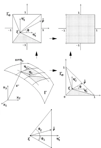
The influence coefficients in the elements Γe, e≠σ can be evaluated using Gaussian quadrature. To determine the influence coefficients containing singularities (element Γσ), one simply has to write the original integral as simple integrals by using directly Taylor expansion around the singular point ξ =' ξ(η1,η2) in polar coordinates, as described in Appendix A3 (see Huacasi, 1999; Guiggiani et al., 1992 and Mantic, 1994). Following Brandão (1987), the one-dimensional CPV integrals are simply computed as the sum of FP integrals, as shown in Appendix A2, (see Hadamard, 1923; Brandão, 1987 and Huacasi, 1999), thus avoiding
regular integral terms as can be seen in Guiggiani et al., 1992; Karami and Derakhshan, 1999.
If quadrilateral plane elements are used, it is convenient to subdivide the singular element into triangles and, following Brandão (1987), the coefficient hifσ becomes a one-dimensional regular integrals which can be evaluated using Gaussian quadrature over the four triangles, i.e:
∑ ∑
= ∆ = − − = 4 1 1 2 1 2 ) ( ˆ ) ( ) ( ˆ ln ) ( g N g g i f if F Fhσ θ θ ωθ
θ ρ
θ θ ρ
θ , (22)
where Ng is the number of Gauss points. For curved elements, expression (22) below holds, being worthwhile noting that Brandão's approach has been used in conjunction with some developments presented by Guiggiani et al. (1992) to transform natural to polar coordinates, that is:
, 2 ) ( ˆ 1 ) ( ) ( ) ( ) ( ) ( ˆ ln ) ( 4
1 1 2
2 1
∑ ∑
= ∆ = − + −= Ng g
g i f
if F F
hσ θ θ ωθ
θ ρ θ β θ γ θ θ β θ ρ θ (23)
where f2 i f2 i
g θ θ θ θ θ
θ= − + − , ρˆ is defined in Appendix A2 and
) ( ), ( ), ( ), ( 2
2θ F θ γ θ βθ
F in Appendix A3. Similarly for
s
iσ, one has:∑ ∑
= ∆ = − − = 4 1 1 2 1 2 ) ( ˆ ) ( ) ( ˆ ln ) ( g N g g i f i f fsσ θ θ ωθ
θ ρ θ θ ρ θ (24) and . 2 ) ( ˆ 1 ) ( ) ( ) ( ) ( ) ( ˆ ln ) ( 4
1 1 2
2 1
∑ ∑
= ∆ = − + −= Ng g
g i f
i f f
sσ θ θ ωθ
θ ρ θ β θ γ θ θ β θ ρ θ (25)
Polar coordinates are used in gσif to evaluate it directly; in this case, the order of the singularity, after the coordinate transformation, is O(ρ−1). Alternatively, gσif can be calculated also by:
∑ ∑
= ∆ = − = 41 11 ( ) 2
) ( ˆ ln ) ( g N g g i f if g
gσ θ θ ωθ
θ β
θ ρ
θ , (26)
where 3 0 0 2 1 4 ) ( A G T g f π φ
θ = .
Validation
In order to show the efficacy of the proposed hypersingular formulation two examples are considered here. The functional nodes (source points ξ) are always located inside the element. As the problems are symmetric, only a quarter or one-half of the domain was discretized. The full domain is taken into consideration by using appropriate reflection of the symmetric elements. To solve the resulting system of linear equations the Gauss method is used.
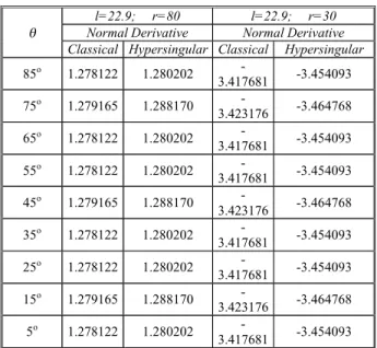
Example 1. The solution of Laplace’s equation in a hollow cylinder with length l =50 units is analyzed now, where the potential on the inner surface is u = 100 and on the outer surfaces is u =0; on upper lateral surfaces pn is considered andx1x2 is a symmetry plane, the boundary is discretized using quadrilateral isoparametric quadratic boundary elements. The results for hypersingular and classical formulation are given in Table 1.
Figure 4. Example 1. Discretization.
Table 1. Normal derivative of potential calculated by classical and hypersingular formulations using quadratic isoparametric elements.
l=22.9; r=80 l=22.9; r=30
Normal Derivative Normal Derivative
θ
Classical Hypersingular Classical Hypersingular 85o 1.278122 1.280202
-3.417681 -3.454093 75o 1.279165 1.288170
-3.423176 -3.464768 65o 1.278122 1.280202
-3.417681 -3.454093 55o 1.278122 1.280202
-3.417681 -3.454093 45o 1.279165 1.288170
-3.423176 -3.464768 35o 1.278122 1.280202
-3.417681 -3.454093 25o 1.278122 1.280202
-3.417681 -3.454093 15o 1.279165 1.288170
-3.423176 -3.464768
5o 1.278122 1.280202
-3.417681 -3.454093
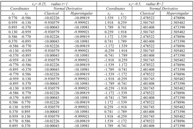
Example 2. In this example, Laplace’s equation is solved in a sphere with a cavity is analyzed. A horizontal symmetry plane has been used so that only half of the boundary had to be discretized. The boundary conditions are: the potentialu = 10 and u = 5 on the interior and exterior surfaces, respectively. The solution obtained is shown in Table 2.
Table 2. Normal derivative of the potential along the intersecting planes: x3=−0.25 with the sphere r=1, and x3=−0.5 with the sphere R=2, calculated by classical and hypersingular formulations using quadratic isoparametric elements.
x3=-0.25, radius r=1 x3=-0.5, radius R=2
Coordinates Normal Derivative Coordinates Normal Derivative
x1 x2 Classical Hypersingular x1 x2 Classical Hypersingular
0.770 -0.586 -10.02226 -10.09819 1.539 1.172 2.478522 2.478896
0.959 -0.130 -9.930579 -9.999921 1.918 0.259 2.501745 2.505482
0.895 -0.370 -10.00043 -10.10981 1.789 0.741 2.481408 2.473390
0.130 -0.959 -9.930579 -9.999921 0.259 1.918 2.501745 2.505482
0.586 -0.770 -10.02226 -10.09819 1.172 1.539 2.478522 2.478896
0.370 -0.895 -10.00043 -10.10981 0.741 1.789 2.481408 2.473390
-0.586 -0.770 -10.02226 -10.09819 -1.172 1.539 2.478522 2.478896 -0.130 -0.959 -9.930579 -9.999921 -0.259 1.918 2.501745 2.505482 -0.370 -0.895 -10.00043 -10.10981 -0.741 1.789 2.481408 2.473390 -0.959 -0.130 -9.930579 -9.999921 -1.918 0.259 2.501745 2.505482 -0.770 -0.586 -10.02226 -10.09819 -1.539 1.172 2.478522 2.478896 -0.895 -0.370 -10.00043 -10.10981 -1.789 0.741 2.481408 2.473390 -0.770 0.586 -10.02226 -10.09819 -1.539 -1.172 2.478522 2.478896 -0.959 0.130 -9.930579 -9.999921 -1.918 -0.259 2.501745 2.505482 -0.895 0.370 -10.00043 -10.10981 -1.789 -0.741 2.481408 2.473390 -0.130 0.959 -9.930579 -9.999921 -0.259 -1.918 2.501745 2.505482 -0.586 0.770 -10.02226 -10.09819 -1.172 -1.539 2.478522 2.478896 -0.370 0.895 -10.00043 -10.10981 -0.741 -1.789 2.481408 2.473390
0.586 0.770 -10.02226 -10.09819 1.172 -1.539 2.478522 2.478896
0.130 0.959 -9.930579 -9.999921 0.259 -1.918 2.501745 2.505482
0.370 0.895 -10.00043 -10.10981 0.741 -1.789 2.481408 2.473390
0.959 0.130 -9.930579 -9.999921 1.918 -0.259 2.501745 2.505482
0.770 0.586 -10.02226 -10.09819 1.539 -1.172 2.478522 2.478896
0.895 0.370 -10.00043 -10.10981 1.789 -0.741 2.481408 2.473390
The tests show good agreements of the results obtained by implementation of our hypersingular with the classical formulation results.
Conclusions
The hypersingular formulation discussed in this paper in terms of CPV is direct and simple. The choice of collocation points located inside the boundary elements allows to compute the free terms through simple expressions. The existence of the Cauchy principal value is explained by showing that divergent terms of the finite part integral cancel each other. The one-dimensional Brandão's technique to calculate the CPV integrals used to solve three-dimensional problems leads to integrals which are regular one-dimensional and that can be calculated by Gaussian quadrature. The numerical solution of the test examples show good agreement with the classical formulation, validating the proposed formulation and the technique used to evaluate the CPV integrals.
Acknowledgements
The first author (W.H.) gratefully acknowledges the financial support provided by CNPq (Conselho Nacional de Desenvolvimento Científico e Tecnológico, Brasil) and FENORTE (Fundação Estadual do Norte Fluminense, Rio de Janeiro).
Appendices
A1. The Second Integral on the l.h.s. of Eq. (5)
Let x be any point of Γε, n(x) a unit normal vector, )}
( ), ( ), (
{τ1ξ τ2ξ nξ an orthogonal coordinate system at the point
ξ, where n(ξ) is normal to Γ at ξ. Then, in spherical coordinates, we have (Fig.1):
) cos , sin sin , cos sin
(ε φ θ ε φ θ ε φ
=
x
and
φ ξ θ φ ξ τ θ φ ξ
τ ( )sin cos ( )sin sin ( )cos )
(x 1 2 n
n = + + .
Thus
φ ξ ξ θ φ ξ τ ξ θ φ ξ τ ξ
ξ) ()) ( () ())sincos ( () ())sinsin ( () ())cos (
(∇xu ⋅nx =∇xu ⋅1 +∇xu ⋅2 +∇xu ⋅n φ
ξ θ φ ξ θ φ
ξ τ
τ1( )sin cos p2( )sin sin pn( )cos
p + +
≡ .
Taking ω(ξ):=n(ξ) we have (n(x)⋅ω(ξ))≡(n(x)⋅n(ξ))=cosφ. Then, changing from orthogonal coordinates to spherical ones, we get:
(
)(
)
∫
∫
∫
ΦΓ
= Γ ⋅ ∇
⋅ ( )
0
2 2
0
2 ( )cos sin
) ( ) ( ) ( ) (
θ π
ε ε θ ξ φ φ φ
ξ ξ
ε
d p
d d
x n u n x
Since for anyθ, 0 ≤ θ ≤ 2π, we have 2
0
lim
πε→
=
(see Fig. 1),then
(
)(
)
( ) 2 1 ) ( ) ( ) ( ) ( 4 3 lim 20 ε ξ ξ
ξ
π ε ε
ε xu n x d pn
n x n = Γ ⋅ ∇ ⋅
∫
Γ → .Similarly, taking ω(ξ):=τ1(ξ) and ω(ξ):=τ2(ξ) we obtain as the limit of this integral values 0.5pτ1(ξ) and 0.5pτ2(ξ) respectively. Thus
(
)(
)
( ) 2 1 ) ( ) ( ) ( ) ( 4 3 lim 20 ε ξ ξ
ξ ω
π ε ω
ε ε p d x n u x n
x ⋅ Γ =
∇ ⋅
∫
Γ
→ .
A2. CPV Computation
Considering parametric coordinates instead of global Cartesian coordinates, one has for the CPV integral:
. | | ) , ( 1 1 1 1 2 1 2 1 ,
∫ ∫
− − ∗= φ η η η η
σ CPV p G d d
hif nn f
When the transformation to polar coordinates (ρ,θ) is used, this integral can be written in FP terms. When a coordinate system with origin point ξ =' (ξ1',ξ2') (image of ξ in parametric transformation) is considered, the following relation holds:
θ ρ ρ η η θ ρ ξ η θ ρ ξ η d d d d = + = + = 2 1 ' 2 2 ' 1 1 sin cos , then
∫ ∫
→ = π ρθθ ρ ε σ ε θ ρ θ ρ 2 0 ) ( ˆ ) (
0 ( , )
lim F d d
hif , (A2.1)
ρ φ π ξ ξ ρ ρ φ θ
ρ i i k k i i f
f n n r n G G r n r O G p F 3 , 2 , 4 )} ( ) )( ( 3 { ) ( | | ) , ( = ∗ = − = − .
Performing the Taylor expansion of F(ρ,θ) (see Appendix A3) one has ) 1 ( ) ( ) ( ) , ( 1 2
2 F O
F
F = + +
ρ θ ρ
θ θ
ρ . (A2.2)
Only the first two terms of the series need to be considered, since
0
lim
→
ρ of the others vanish.
Note that there is no need to be restricted to the first two terms of the Taylor series; in fact, any order of singularity can be dealt with following the approach presented here. Then-1 first terms of the Taylor expansion (A2.2) in polar coordinates can be used to remove singularities of order n-1, whenever u∈Cn−2,α in the neighborhood ofξ. This idea was used previously by Karami and Derakhshan (1990) in order to generalize the procedure presented in Guiggiani et al. (1995).
Now, from (A2.1) and (A2.2) one obtains:
. ) ( ) ( lim 2 0 ) ( ˆ ) ( 2 2 1
0
∫ ∫
+ = → π ρθ
θ ρ ε σ ε θ ρ ρ θ ρ θ d d F F hif
For plane elements, following Brandão (1987), one can write:
θ θ ρ θ θ ρ θ π
σ F d
F
hif
∫
− =2 0 2 1 ) ( ˆ ) ( ) ( ˆ ln ) ( with θ θ ρ θ θ ρ θ π
σ f d
f
si
∫
− =2 0 2 1 ) ( ˆ ) ( ) ( ˆ ln ) (
and expressions (21) and (23) are obtained. When curve elements are used, taking advantage of the results of Guiggiani et al. (1992):
θ θ ρ θ β θ γ θ θ β θ ρ θ π
σ F F d
hif
∫
+ − =2 0 2 2 1 ) ( ˆ 1 ) ( ) ( ) ( ) ( ) ( ˆ ln ) ( with θ θ ρ θ β θ γ θ θ β θ ρ θ π
σ f f d
si
∫
+ − =2 0 2 2
1 ˆ( )
1 ) ( ) ( ) ( ) ( ) ( ˆ ln ) ( .
A3. Taylor Expansion of the Integrand
When:
( ) ( )
, f , f,Fρθ = ρθφ
3 , , 4 )} ( ) )( ( 3 { | | ) , ( r n G G r n r G p
f nn i i k k i i
π ρ ξ ξ ρ θ
ρ = ∗ = −
and using polar coordinates, the Taylor expansion of each term is:
) ( 2
3
, ρ ρ
ξ O A B A A A B A A r x
ri i i i i i k k +
− + = − = , θ η θ
η1η=ξ'cos ∂ 2η=ξ'sin
∂ + ∂
∂
= i i
i x x A , , 2 sin cos sin 2 cos 2 ' 2 2 2 ' 2 1 2 2 ' 2 1 2 θ η θ θ η η θ
η η=ξ η=ξ ∂ η=ξ
∂ + ∂ ∂ ∂ + ∂ ∂
= i i i
i
x x
x B
whereA and B are the magnitudes of vectors having components Ai and Bi. For the remaining components:
) ( A B A n 1 A
rn n n k2k+O n+2
+
=ρ ρ ρ ,
ρ ρ ρ 1 3 1 1 5 2 3 3
3 = − A +
B A A r k k , ) ( O G G ) ( o sin G cos G ) ' ( G
G k K
' k
' k k
k 2 0 1 2
) ( )
( sin cos
) '
( 2 0 1 2
' 2 ' 1
ρ ρφ φ ρ θ η φ θ η φ ρ ξ φ φ
ξ η ξ
η
O
o f f
f f
f
f + = + +
∂ ∂ + ∂
∂ + =
= =
,
) ( ) ( ) (
) ( 3 ) ( ) )( (
3, 2 0 1 1 ξ 0 ξ
ξ ρ ξ
ξ k k i i i i k k k k i i i i i
i BG AG Gn Gn
A n A n
G G r n
r −
+ −
=
− ,
) ( 0
1 Gini ξ
T = , T2=Aini(ξ),
) ( 1
3 Giniξ
T = ,
1
0 k k
k
kG AG
B
P= + ,
( )
− −
+ +
− −
= k k f f f f
f
T T P A T
A T A
B A
A T
F 2 0 30 11
2 3 0 1 5 3
3 0 1
3 1 3
1 4
1
, φ φ φ φ
ρ ρ
φ π θ
ρ ,
( )
−
+ −
= 5 1 3 22 3
1 3
1 3
4 1
T P A T A T A
B A
f k k
π
θ ,
( )
132 4
1 A T f
π
θ = ,
f f
A T f
F 1
3 1 0 1 1
4 ) ( )
( φ
π φ θ
θ = + ,
f f F2(θ =) 2(θ)φ0 .
Expressions above are the only one required when flat elements are employed. If the element is not flat, the following expansion for
ε =
r is required:
) ( 2
2 ρ
ρ ρ
ε O
A B A
A+ k k +
= ,
) ( ) ( ) ( )
(θ εβθ ε2γ θ ε3
ρ
ρ= ε = + +O ,
where
A 1 ) (θ =
β and
4
) (
A B Ak k
− = θ
γ .
References
Brandão, M.P., 1987, "Improper Integrals in Theoretical Aerodynamics: The Problem Revisited", AIAA Journal, Vol.25, pp.1258-1260.
Brebbia, C. A., Telles, J. C. F. and Wrobel, L. C., 1984, "Boundary Element Techniques", Springer-Verlag, Berlin, 464 p.
Guiggiani, M., Krishnashamy, G., Rudolphi, T.J. and Rizzo, F.J., 1992, "A General Algorithm for the Numerical Solution of Hypersingular Boundary Integral Equations", Journal of Applied Mechanics, Vol.159, pp.604-614.
Guiggiani, M., 1995, "Hypersingular Boundary Integral Equations Have an Additional Free Term", Computational Mechanics, Vol.16, pp.245-248.
Hadamard, J., 1923, "Lectures on Cauchy's Problem in Linear Partial Differential Equations", Yale Univ Press, New Haven, USA.
Huacasi, W., 1999, "A Hypersingular BEM Formulation for 3-D Potential Problems", D.Sc. Thesis COPPE/UFRJ, Rio de Janeiro, Brasil, 107 p.
Karami, G. and Derakhshan, D.,1999, "An Efficient Method to Evaluate Hypersingular and Supersingular Integrals in Boundary Integral Equations Analysis", Engineering Analysis with Boundary Elements, Vol.23, pp.317-326.
Kolm, P. and Rokhlin, V., 2001, "Numerical Quadratures for Singular and Hipersingular Integrals", Computers and Mathematics with Aplications 41, pp.327-352.
Krishnasamy G., Rizzo F.J. and Rudolphi, T.J., 1992, "Continuity Requirements for Density Functions in the Boundary Integral Equation Method", Computational Mechanics, Vol.9, pp.267-284.
Kutt, H.R.,1975, "The Numerical Evaluation of Principal Value Integrals by Finite-Part Integration", Numer. Math., Vol.24, pp.205-210.
Mansur, W.J., Fleury, Jr. and Azevedo, J.P.S, 1997, "A Vector Approach to the Hypersingular BEM Formulation for Laplace’s Equation in 2D", The International Journal of BEM Communications, Vol.8, p.239-250.
Mantic, V., 1994, "On Computing Boundary Limiting Values of Boundary Integrals with Strongly Singular and Hypersingular Kernels in 3D BEM for Elastostatics", Engineering Analysis with Boundary Elements, Vol.13, pp.115-134.
Mantic, V. and Paris, F., 1995, "Existence and Evaluation of the Two Free Terms in the Hypersingular Boundary Integral Equation of Potential Theory", Engineering Analysis with Boundary Elements, Vol.16, pp.253-260.
Mikhlin, S. G., 1957, "Integral Equations and their Applications to Certain Problems in Mechanics, Mathematical Physics and Technology", Pergamon Press, London New York.
Pinciroli, G. A., 1995, "The MEC3D to Analyse 3-D Potential Problems by the BEM", M.Sc. Thesis, COPPE/UFRJ, Rio de Janeiro, Brazil.
Sladek, V. and Sladek, J., 1996, "Regularization of Hipersingular Integrals in BEM Formulation Using Various Kinds of Continuous Elements", Engineering Analysis with Boundary Elements, Vol.17, pp.5-18.
Tanaka, M., Sladek, V. and Sladek, J., 1994, "Regularization Techniques Applied to Boundary Element Methods", ASME, Appl. Mech. Rev., Vol.47, No. 10, pp.457-497.