www.nat-hazards-earth-syst-sci.net/10/429/2010/ © Author(s) 2010. This work is distributed under the Creative Commons Attribution 3.0 License.
and Earth
System Sciences
An approach to combine radar and gauge based rainfall data under
consideration of their qualities in low mountain ranges of Saxony
N. Jatho, T. Pluntke, C. Kurbjuhn, and C. Bernhofer
Institute of Hydrology and Meteorology, Department of Meteorology, Technische Universit¨at Dresden, Dresden, Germany Received: 29 April 2009 – Revised: 12 February 2010 – Accepted: 20 February 2010 – Published: 11 March 2010
Abstract.An approach to combine gauge and radar data and additional quality information is presented. The development was focused on the improvement of the diagnostic for tempo-ral (one hour) and spatial (1×1 km2) highly resolved precip-itation data. The method is embedded in an online tool and was applied to the target area Saxony, Germany. The aim of the tool is to provide accurate spatial rainfall estimates. The results can be used for rainfall run-off modelling, e.g. in a flood management system.
Quality information allows a better assessment of the in-put data and the resulting precipitation field. They are stored in corresponding fields and represent the static and dynamic uncertainties of radar and gauge data. Objective combination of various precipitation and quality fields is realised using a cost function.
The findings of cross validation reveal that the proposed combination method merged the benefits and disadvantages of interpolated gauge and radar data and leads to mean es-timates. The sampling point validation implies that the pre-sented method slightly overestimated the areal rain as well as the high rain intensities in case of convective and advective events, while the results of pure interpolation method per-formed better. In general, the use of presented cost function avoids false rainfall amount in areas of low input data quality and improves the reliability in areas of high data quality. It is obvious that the combined product includes the small-scale variability of radar, which is seen as the important benefit of the presented combination approach. Local improvements of the final rain field are possible due to consideration of gauges that were not used for radar calibration, e.g. in topographic distinct regions.
Correspondence to:N. Jatho ([email protected])
1 Introduction
Precipitation is the most important parameter for hydrol-ogists and water resource engineers, especially since fre-quency and intensity of heavy rains increased in Saxony (Bernhofer et al., 2008) which seems to be an ongoing trend (Alcamo et al., 2007). Special regard is given to mountain-ous catchment areas, where steep slopes and short flow paths cause local flash floods. Thus, an efficient real-time flood forecasting requires improvements of the applied hydrologi-cal models as well as of the precipitation input.
Many national and international studies focus on the de-termination of the most accurate spatial rainfall product. In situ measurements are used to obtain the actual amount of rainfall at individual locations. Nowadays, it is possible to provide the data in a very high temporal resolution (up to one minute). But, as discussed by Cherubini et al. (2002) as well as by Ballester and Mor´e (2007), an accurate rep-resentation of the spatial distribution of rainfall requires a high-resolution network. Curtis (1996), Fuchs et al. (2001), Michelson (2004) and Sevruk (2004) analysed problems of local measurements of less than one hour, daily and monthly resolutions. Neˇspor and Sevruk (1999) investigated wind er-rors and showed that the wind erer-rors strongly vary with at-mospheric conditions and precipitation type. Furthermore, the location of gauges strongly influence their representative-ness, which is also known as site error (German and Joss, 2001; Villarini et al., 2008). As a result, spatially limited high rain intensities of short duration (convective precipita-tion) can be determined or remains undiscovered. Advec-tive precipitation covers larger areas and is characterized by a more homogeneous distribution of rain intensity (Houze, 1997) and thus is mostly detected by gauge measurements.
made about spatial correlations of the considered data. Sta-tistical methods analyse the variances between two values as well as the distance between them. Hinterding (2003), Haberlandt et al. (2005), and Pluntke et al. (2010) apply krig-ing methods to small and large-scale rainfall events with res-olutions from one hour to several days. These methods show good results regarding the delineation of precipitation areas, but not for the internal variability within the precipitation fields and the rain intensities. Here, the quality of interpo-lation results strongly depends on the station density.
The importance of radar-born precipitation products as input for hydrological modelling increased during the last years, because of their high spatial and temporal resolution. Aniol and Riedl (1979), Kr¨amer (2008) as well as Villarini and Krajewski (2010) discussed measurement errors like un-certainties in the interpretation of the radar signal as well as the influences of atmospheric parameters (e.g. temperature and wind) and topography. The correction or minimisation of these errors is a focus of ongoing radar research for the Nim-rodradar system of the United Kingdom (temporal resolu-tion: 5 and 15 min, spatial resoluresolu-tion: 2 and 5 km), Harrison et al. (2000) and Germann et al. (2009) analysed problems of radar measurements as well as possibilities for correction, e.g. a scheme for removal of spurious radar echoes or the use ofensembleradar precipitation estimates. The correction of errors like wind speed shifted hydrometeors in case of heavy rainfall is still limited (Delrieu et al., 2000).
Harrison et al. (2000), Bartels (2004), Berne et al. (2004), and Kr¨amer (2008) reported that the combined products of radar and rain gauges contained fewer observational errors than the individual input datasets. Harrison et al. (2000) achieved a reduction of theroot mean squaredifference be-tween gauge and radar measurements of 30%. Borga et al. (2002) showed that a successful combination of radar and rain gauge data is possible only if range effects are ad-justed in the radar rainfall observations. Seo and Breiten-bach (2002) combined radar and gauge measurements within a real-time procedure leading to a reduction of the systematic radar bias in the cold season between 16 and 27% and in the warm season between 17 and 26% as well as a reduction of themean squared errorbetween 34 and 46% and between 23 and 31%.
The combination of spatial radar and gauge data requires the application of data assimilation concepts. Observations are combined with so-calledBackground(first guess) infor-mation. TheBackground results from climatic conditions, the output of a previous analysis, simulations of a forecast model (Bouttier and Courtier, 2002) or radar data (Pereira Fo and Crawford, 1999). The actual analysis output is consid-ered to be the best estimate. Further analysis steps optimise the estimations with the objective to minimise data uncer-tainties. For more details see Bouttier and Courtier (2002) as well as Wergen (2002). Thestatistical objective analysis (SOA) belongs to the group of assimilation methods. Back-ground-fields are used to reduce the error variances of
ob-served gauge measurements. Pereira Fo and Crawford (1999) adopted the SOA-method and used temporally and spatially highly resolved radar data as Background. Gerstner and Heinemann (2008) adopted these studies for real-time pre-cipitation estimation for short time intervals.
The aim of our work is to combine spatial gauge and radar data under consideration of their qualities and provide a more accurate rainfall diagnostic product for hydrological mod-elling in real-time. During operation, our tool determines the current precipitation type based on radar precipitation fields. Errors of the data which could not be treated beforehand, re-spectively uncertainties, are considered within data specific quality fields. In a cost function we combine the grid based precipitation and quality fields by weighting the different rain retrievals dependent on their quality. The algorithm gener-ates a grid based precipitation and quality field.
Our approach represents a modification of SOA. We com-bined interpolated gauge data (provided by the German Weather Service, DWD, and the Saxon State Ministry of the Environment and Agriculture) from a relatively dense network (observation) with hourly radar precipitation data (Background). The radar data (RADOLAN) are already online-adjusted with gauge data from the DWD (Bartels, 2004). The use of the additional gauge information enhances the reliability of rain amounts given by radar data. The com-bination is realised by the online precipitation diagnosis tool, developed for this study.
The current study is divided into five sections: Section one gives an overview about state of the art of precipitation analysis and limitations using radar and gauge data for real-time precipitation estimation. Within this context the section presents the motivation, aims and approaches of the present study. Section two provides information about the study area as well as the investigated precipitation data. Section three introduces to the applied methodologies of rainfall diagnos-tic with emphasis on rainfall classification, statisdiagnos-tical assess-ment of rainfall data, quality analysis of input data and an approach to combine several precipitation and quality prod-ucts. The results of the study for selected time periods and two case studies are presented in chapter four. In the last section (Sect. 5) the results are discussed and an outlook for future research is given.
2 Study area and data
This section gives an overview about the study area, the pre-cipitation sources and the investigated rainfall events. 2.1 Study area
∆ rain gauge, hourly measurement interval ○ rain gauge, 1 minute measurement interval
Fig. 1. Investigation area covered by the radar station Dresden-Klotzsche and adjacent stations of Bavaria, Thuringia, Saxony-Anhalt and 1-min as well as hourly gauge data. The hourly stations (with a few exceptions) are used for the online calibration of radar data.
The Fichtelberg (1214.6 m) is the highest mountain in the study area. Focus of our investigations lies on the hilly re-gions and the low mountain ranges. Here, the flood prob-lem is more pronounced, because precipitation intensities are often higher, and steep topographic gradients cause surface runoff. Floods of mountainous catchments are characterised by pronounced flood peaks and short lead time.
2.2 Data
2.2.1 Rain gauges
We used precipitation data from 67 rain gauge stations within an area of about 18 000 km2. The data were provided by the DWD and the Saxon State Ministry of the Environment and Agriculture. The temporal resolution ranges from one minute to one hour. Data with higher temporal resolutions were accumulated to hourly data. Most precipitation data were provided in real-time. Measurements were not corrected for
2.2.2 Weather radar
Rainfall measurements by radar provide quantitative rainfall information with high temporal and spatial resolution. In general, radar precipitation data are no direct measurements, only the reflection of electromagnetic waves from falling droplets within a certain volume is determined. The most commonly used method to describe the relationship between reflectivity (Z) and rain rate (R) is the so-calledZ-R rela-tionship(Eq. 1), where the coefficientsaandbare empirical. They vary depending on the given rainfall situation.
Z=aRb (1)
High rain intensities result in a severe attenuation of the radar signal (Rinehart, 2004). Thus, within a convective cell radar measurements can be insufficient.
The DWD provides hourly precipitation data based on measurements with aC-band Dopplerradar. Shadowing ef-fects, rain intensity adaptedZ-R relationships, statistical clut-ter filclut-tering and other features are handled within an online calibration process (Bartels, 2004). In addition, derived pre-cipitation intensities are online calibrated with ground sta-tion measurements. The so-called RADOLAN RW prod-uct represents a final precipitation prodprod-uct, which is hourly available as a composite consisting of 16 German and some foreign radar stations (e.g. Nancy/France). An area-wide coverage of radar data is provided for Germany and the adjacent areas with a spatial resolution of 1×1 km2 (Bar-tels, 2004). The radar station Dresden-Klotzsche (13.75◦E and 51.13◦N) covers the main part of the investigation area (Fig. 1). The inclusion of adjacent station data of the fed-eral states Bavaria, Thuringia and Saxony-Anhalt allows for a complete coverage of the study area.
The temporal offset of 10 min between gauge and radar observations has to be noticed. We used hourly gauge data (e.g. 01:00 UTC), 1 min highly resolved data (aggregated to hourly sums) and combined them with RADOLAN data, which were available 10 min before (e.g. 00:50 UTC). 2.3 Considered rainfall events
For diagnostic we chose mostly heavy rainfall events from May to August 2006 and January 2007, a 16 days lasting period from 26 July to 11 August 2006 as well as a three month period from 1 May to 31 July 2009. We classified the events into convective or advective cases and investigated the precipitation data and their characteristics. Two case studies were analysed in detail (convective: 16 June 2006, 14:00 UTC, advective: 27 May 2006, 17:00 UTC).
3 Methodology of rainfall diagnostic
In this section, we present the applied method for rainfall classification. We studied the different errors in rainfall es-timation methods based on gauge and radar measurements,
Table 1. Definition of Wetted Area Ratio (WAR) and Area Ratio of rain intensity up to 10 mm/h (10AR) values for assignment of different precipitation types: convective (con.) and advective (ad.).
Precipitation WAR [–] 10AR [–]
type
con. 0.0<WAR≤0.5 0.05<10AR≤0.7
ad. 0.25<WAR≤1.0 0.0<10AR≤0.05
applied a statistical assessment and introduce an approach to handle uncertainties. The spatial gauge and radar precipi-tation data are combined taking into account their qualities within a cost function.
3.1 Rainfall classification
An accurate classification of the rainfall event into convective (here: in connection with vertical airflow, accompanied by local short-term showers, thunderstorms) or advective (here: in connection with horizontal airflow, large-scale long-term precipitation with moderate intensities) is in our opinion fun-damental for a successful rainfall diagnostic. Radar data are often used for rainfall classification (Sempere-Torres et al., 2003; Ehret, 2003) and the established methods work almost reliable. We chose the radar based classification method, de-veloped by Ehret (2003) and calculated the parameters Wet-ted Area Ratio (WAR) and the Area Ratio (AR) of rain in-tensity with more than 10 mm/h (10AR) for the study area. WAR defines the ratio of the area with precipitation inten-sities greater than 1 mm/h to the whole raining area of the considered radar image, whereas 10AR is the proportion of WAR, where precipitation exceeds 10 mm/h. Both parame-ters are used to define, which rainfall type dominates the cur-rent event. Ehret (2003) distinguished six rainfall types and we simplified this method to a coarse classification discrim-inating only convective or advective precipitation (Table 1). Attention was paid, that no undefined parameter constella-tions arise to guarantee the system stability of our online tool. Thus, advective type is assigned as default, if param-eter WAR and 10AR do not allow explicit classification.
The proof of temporal stability of the event classifica-tion using WAR and 10AR is done by means of five sta-bility indices from radio sounding data (stations: Linden-berg, Essen, Stuttgart and Meiningen). The results are com-pared with the classification of WAR and 10AR for an area of 120×120 km2around four radar stations (Berlin, Essen, T¨urkheim, Neuhaus). The choice of investigated areas takes into account the influence of topography on the sounding data (Steinheimer and Haiden, 2007).
Table 2.Thresholds for stability indices Convective Available Po-tential Energy (CAPE), K Index (KI), Lifted Index (LI), Showalter Index (SI) and Total Totals Index (TT) for the assignment of differ-ent precipitation types: convective (con.) and advective (ad.).
Stability Threshold [–] index
con. ad.
CAPE >500 ≤500
KI >27 ≤27
LI <–1 ≥–1
SI <–1 ≥–1
TT >52 ≤52
Index (LI), Showalter Index (SI) and Total Totals Index (TT) (Peppler, 1988; Van der Velde, 2007). The thresh-olds for the five sounding parameters (Table 2) are needed for the description of the atmospheric condition. They are derived based on the studies of Kunz (2007), Dimitrova et al. (2009), Peppler (1988), Pineda et al. (2007), Queralt et al. (2008), and S´anchez et al. (2003). The sounding indices at 00:00 UTC and 12:00 UTC were checked against the corre-sponding radar results (hh:mm-50 UTC) for the period from 1 May to 31 July in 2009.
3.2 Statistical assessment of data
The main problems of a grid based rainfall diagnostic are the measurement principles and the spatial representatives of estimated gauge and radar rainfall data as well as the com-parability of both data sources. Falling rain drops can be detected by radar, although they never reach the ground. Fur-thermore, the influence of wind drift can lead to an increasing horizontal drift of hydrometeors. The influences of several atmospheric errors of gauge measurements are discussed in detail by Neˇspor and Sevruk (1999), Michelson (2004), and Sevruk (2004). Collier (1999) and Quirmbach (2003) anal-ysed the influence of these errors on radar data. We assume that radar data can complement gauge detected rain (i.e. in case of convective event). In due consideration of meteoro-logical influences on radar data, we implemented an assess-ment based on the deterministic categorical scores BIAS and Heidke Skill Score (HSS) to discriminate, whether radar data should be used as additional information at gauge stations.
In order to detect spatial offsets between, radar and gauge measurements, we examined the 3×3 pixel neighbourhood of each gauge station. We assumed the radar rain value with the smallest difference to the gauge value to be the corre-sponding rain value. Further, we used the deterministic cate-gorical scores BIAS and HSS, as described in Wilks (2006), for the determination of the data quality. The basis of these parameters is ayes-no statement. We adjusted the scores,
Table 3. 2×2 contingency table for the determination of statistical scores BIAS andHeidke SkillScore (HSS).
Radar Gauge
(derived) (observed)
Yes No
Yes a b
No c d
which were originally developed for forecast systems and use gauge measurements as observed and radar values as derived (original: forecasted) precipitation data. The grid based anal-ysis of possible combinations between gauge and radar mea-surements requires a 2×2 contingency table (Table 3). Here, BIAS defines the ratio between the number of detected radar measurements and gauge measurements (Eq. 2):
BIAS=a+b
a+c (2)
with:
a= hit: rainfall is measured by gauge and radar. b= false alarm: rainfall is measured only by radar. c= miss: rainfall is measured only by gauge.
d= correct negatives: rainfall is not measured by gauge and radar.
An unbiased distribution is given when BIAS is equal to 1. If the analysis detected more radar data above the thresh-old than gauge values (higher average percentage of false alarms), the BIAS is greater than 1 and describes an overesti-mation of gauge measurements. With BIAS less than 1, more gauge measurements were detected (higher average percent-age of misses) and radar underestimated gauge data.
The HSS (Eq. 3) is basically defined by the assumption of the proportion of hits. According to this definition, HSS in this study assumes that radar data are a result of a random process, but they are statistical independent from observed gauge data. HSS ranges from –1 to 1, where 1 reflects the best analogies of hits, false alarms, misses and correct nega-tives of radar and gauge data. Zero means radar is equivalent to gauge (Wilks, 2006) and negative values indicates that the chance forecast (here: radar) is better.
HSS= 2(ad−bc)
3×3 and 4×4 contingency tables are implemented. The defi-nition of hits, false alarms, misses and correct negatives was adapted. Consequently, the parameters specify whether radar and gauge data, only radar data, only gauge data or no cor-responding radar and gauge data were found within current precipitation range.
To get an impression of mean rain characteristic and to define, whether a skill score indicates a good agreement be-tween radar and gauge data, we analysed the chosen events (420 h, Sect. 2.3) and calculated the BIAS and HSS. Gauge data, which were used for the radar calibration process, were omitted. The empirical derived limits are the temporal mean over all precipitation ranges of the investigated events. Our analysis resulted in a BIAS between 0.96 and 1.40 and a HSS higher than 0.55 for convective events and a BIAS be-tween 0.91 and 1.45 and a HSS higher than 0.59 for advec-tive events. BIAS values are in the range of the findings of Sokol (2003). No reference values were found for HSS values.
We analyse the rain events (Sect. 2.3) and found that on average the percentage of extended areas for advective and convective events is similar. Areas of convective events are less appropriate sampled (HSS: 0.55) than areas of advective events (HSS: 0.59). BIAS is more skewed in case of advec-tive events. The reasons were found in higher differences between compared data couples (right-skewed: higher radar values, left-skewed: higher gauge values). We applied the thresholds for current work, because we assumed the anal-ysed events as representative for real-time operation. If BIAS and HSS within the different ranges of 3×3 or 4×4 contin-gency table do not fulfil the mentioned criteria, agreement between radar and gauge data is marginal. As a result, no radar data are used to enhance gauge data at the specific lo-cation (for particulars see Sect. 3.4).
3.3 Quality analysis
The quality of both precipitation products was considered in this work as a static part capturing all uncertainties that are permanent and independent from the current conditions (Qstat). On the other hand the dynamic part of uncertainty was determined, that means errors of the actual dataset were accounted for. Quality is expressed within the range from zero to 100%, whereas 100% represents for gauge as well as radar data the best precipitation value. Germann and Joss (2001) showed clearly (by using radar data), that repre-sentativeness of point observations depend on the degree of spatial variation (depending on time, location and integration time) and uncertainty of the single measurement.
3.3.1 Gauge quality
Spatial representativeness of rain gauges is regarded as the static part of the quality. It is a known fact, that
precipita-tion measured with a gauge is less representative for its sur-rounding in case of convective events compared to advective events. Furthermore, topography determines spatial rep-resentativeness of gauges. There are various processes in mountainous regions that cause a higher spatial variability. The most important processes are topographic lifting of air masses and enhanced precipitation on the windward side of the mountain, the rain shadow on the leeward side, the di-urnal convection, the seeder-feeder-effect at the windward sides of small hills etc.
There are only few investigations that focused on the spa-tial representativeness of rain gauges. For daily precipitation values Sevruk (2004) states that gauge measurements repre-sent an area of two kilometres in diameter in flat regions and of one kilometre in mountainous regions. Representative-ness of hourly and even higher resolved values can be much smaller, especially for thunderstorms and on top of moun-tains. For hourly values Gebremichael and Krajewski (2004) showed that correlation between gauges that are for example 2 and 8 km separated from each other dropped from 0.8 to 0.4. Considering all rainfall events with more than 1 mm/h, Moreau et al. (2009) found that correlation reduced to 0.7 within a distance of 6 km. For events with more than 3 mm/h rainfall correlation decreased to 0.4. The results of Moreau et al. (2009) and Gebremichael and Krajewski (2004) base on a limited database of one or two months. Furthermore, convective systems of Florida (USA), the Amazonas region, France and Germany are not fully comparable.
A clear limited extension of shower cells was published by the German Weather Service (DWD, 1981) for a Ger-man radar station. So, 80% of the investigated rain cells with rain intensities of 1 mm/min and 97% of the rain cells with 2 mm/min were smaller than 4 km2. No investigation about the representativeness of gauge measurements is known for our study area.
Table 4. Static quality of rain values in dependence on distance to gauge, topography, and rain event type (convective: con. and advective: ad.).
Qstat[%] Distance [km]
Hilly region Mountainous region
con. ad. con. ad.
100 0.65 2.0 0.35 1.0
70 1.4 4.0 0.65 2.0
40 2.7 8.0 1.0 3.0
10 ≥3.7 ≥11.0 ≥2.0 ≥6.0
To account for the dynamic part of gauge quality, we estab-lished a plausibility check for precipitation data of a temporal resolution between 1 and 60 min. The following criteria were applied:
I. Threshold check for physically meaningful values. Up to mean values of 8 mm/1 min, 40 mm/10 min and 90 mm/60 min the data are assigned withQdyn=100%. Rain values are flagged with zero for maximum values above 20 mm/1 min, 60 mm/10 min or 120 mm/60 min. In-between,Qdynis the difference of maximum quality and the weighting of actual rain amount.
II. Test of constant intensities of consecutive time steps. Highest quality is allocated for up to six consecu-tive time steps of low rain intensities (0.1 mm/1 min, 1 mm/10 min, 1 mm/60 min). If the values have been unchanged for more than eight times, they are indicated as zero. In-betweenQdynis reduced linearly. The num-ber of plausible constant intensities decreases with in-creasing precipitation amounts. E.g., if a value above 3 mm/1 min is detected more than two times, it is indi-cated withQdyn=0%.
III. Test of physically meaningful differences between con-secutive time steps. The criteria differ depending on the season (summer: April–September, winter: October– March). Highest quality is assigned to differences up to 4 mm/1 min (summer), 25 mm/10 min (summer), 3 mm/1 min (winter) and 10 mm/10 min (winter). Low-est quality is assigned to values above 8 mm/1 min (summer), 35 mm/10 min (summer), 7 mm/1 min (win-ter) and 20 mm/10 min (win(win-ter). In-between, Qdyn is reduced linearly.
IV. Test of minimal duration of a precipitation event above a certain threshold. LowestQdyn is assumed for rain amounts above 1 mm/h and a duration of more than 2 min.
V. Threshold test for physically meaningful hourly values for the past 60 min (same criteria as described in plausi-bility check [I]).
Data with a resolution of 10 min were not checked for teria (IV). Hourly data were additionally not checked for cri-teria (III) and (V). Mean and maximum thresholds are the result of a literature review (e.g. Bartels et al., 2005) and an analysis of long-term datasets (1 min and 10 minute: 2005– 2008, 1 h: 1992–2008). We defined threshold ranges and no kick out criteria (worst quality is defined as zero). It is diffi-cult to fix thresholds that reflect the conditions of the domain. It entails the risk that thresholds, which are too low, could cause an elimination of extreme values and thresholds, which are too high, would not allow detecting data errors. Data were aggregated to hourly values, whereas missing values were replaced. Here, a minimum of 49 values for 1-min and 5 for 10-min values was required to aggregate them to an hourly value. A quality in the range of zero and 100% was assigned to hourly data as a result of the plausibility check. Only precipitation data with a quality (Qdyn) greater than zero were considered for further analysis.
The localQdynwas used to enhance the spatial station rep-resentativenessQstat. Here, the static quality field was re-duced by the difference that resulted from the differences of Qdyn andQstat at the stations. A multiplicative procedure to combine both qualities would result in somewhat higher quality. Because we had no mean to validate the performance of both procedures, we chose the subtraction procedure. An hourly quality field resulted from this combination (compare Figs. 9b and 11b).
3.3.2 Radar quality
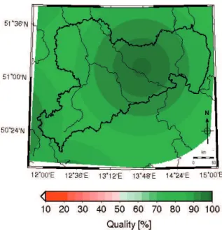
The accurate interpretation of the reflectivity signal is essen-tial for the quality of rainfall estimation (Rinehart, 2004). The provided radar data (Sect. 2.2.2) already passed sev-eral procedures (e.g. correction of default values, tion of attenuation based on precipitation intensity, correc-tion of topographic influences, improvedZ-R relationship). But the adaption of correction methods is still difficult for the real-time processing of data (Bartels, 2004). Therefore we quantified potential errors within a quality field. The static field (Qstat) results from the attenuation effect (de-creasing data quality with in(de-creasing distance to the radar station). Combining the results of Delrieu et al. (2000), Kr¨amer (2008), and Gerstner and Heinemann (2008) a qual-ity reduction of 20% for a maximum distance of 128 km is assumed for the applied radar data and stored into theQstat field (Fig. 2).
The dynamic quality criterion (Qdyn) was derived from ac-tual differences between gauge and radar data. The steps to derive the dynamic quality field were:
Fig. 2.Static quality field (Qstat) of radar data.
to the gauge value was assumed to be the corresponding value.
2. An empirical quality between 10 and 100% was as-signed to encountered differences between radar and gauge data. We allocated a quality of 100% for dif-ferences between gauge and corresponding radar data below 10%. For more than 40% difference, a quality of 10% was assigned. The low data quality is assigned to take into account, that the statistical errors also increase (Sokol, 2003). In-between values were calculated by a linear approach at the sampling points.
3. The empirical qualities were interpolated applying In-verse Distance Weighting (IDW) onto the radar grid and represent the dynamic quality fieldQdyn.
The validity of Qdyn Radar depends on the number of available gauge stations. If only a few gauges deliver values for an actual event, the interpolation of the empirical quali-ties is critical. Due to the high spatial variability of rainfall and the complex error characteristic of radar data, we assume that the differences between radar and gauge are only valid for a limited area around the gauge. We followed the study of Ballester and Mor´e (2007) and replacedQdyn byQstatif less than eight stations are available.
3.4 Data combination
We combined our precipitation and quality fields within a SOA. As described by Pereira Fo and Crawford (1999), radar data were used asBackgroundand the rain gauge data as the observed part. Similar to Gerstner and Heinemann (2008) we
modified the basic analysis equation of the SOA technique (cost function) for our real-time requirements:
P (x,y)=
n
X
i=1
(Pi(x,y)wi(x,y)) (4)
Precipitation in a grid cellP(x, y)is calculated as the sum of the products of different grid based precipitation sources (Pi)
with their corresponding weighting fields (wi). The
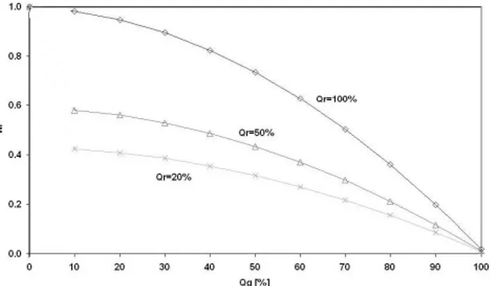
minimi-sation of background error-variance within a cross correla-tion (between gauge and radar data) as described by Pereira Fo and Crawford (1999) was replaced by the application of the derived quality fields (radar quality: Qr, gauge quality: Qg). The relations between radar (wr) and gauge weighting (wg) depending onQrandQgare described in detail by the following equations:
wr(x,y)=k((100−Qr)/10)
l Q2g+m Qg+n
(5) wg(x,y)=1−wr(x,y) (6) Equation (5) represents a quadratic function, whereas the first term represents the adjustment of the weighting function de-pending on the actual radar quality. The second term in-cludes the weighting in dependence on gauge quality. When-ever one rainfall product (radar or gauge data) was unknown or failed, that means its quality equals zero, the remaining product was weighted with one (Eqs. 5 and 6). We tested the functionality of Eq. (5) based on several couples of radar and gauge data with hourly resolution, for different atmo-spheric conditions and distances, and determined the empir-ical parametersl,m,n, andkfor convective situations (with l=−0.00007, m=−0.0002, n=0.9932, k=0.9) and for ad-vective situations (withl=−0.0001,m=−0.0008,n=0.9994, k=0.9). For example, Eq. (5) results in a higher weighting of radar data for convective than for advective events, caused by the limited representativeness of gauge measurements.
Fig. 3. Radar weights (wr) based on radar (Qr) and gauge (Qg) qualities in case of convective precipitation events.
and no radar data are available or the values of BIAS and HSS do not exceed prescribed limits, radar weighting is set towr=0. Furthermore noticeable is the step of the curves for Qgless than 10% in Figs. 3 and 4. This gap is to ensure that in case of very poor or missing gauge data the sum of the weightings equals one.
The final quality product Q(x,y) can be calculated us-ing Eq. (4), just replacus-ing Pi(x,y) with the quality fields
Qi(x,y).
We used the cross validation method for the analysis of the applied methods. The gauge measurements (stations are excluded, which are part of the Radolan procedure) were directly compared with pure interpolated gauge data, pure radar data and the combined precipitation value. We used the BiasCV (not to be confuse with the BIAS skill score mentioned before) (Eq. 7) and the root-mean-squared error (RMSE) (Eq. 8) as criteria. Low BiasCV values indicate a good reproduction of the average areal precipitation, whereas low RMSE values reflect, that higher rain intensities were captured well. In Eqs. (7) and (8)pi describes the estimated
andoithe observed value.
BiasCV=1
n
n
X
i=1
(pi−oi) (7)
RMSE=
v u u t 1 n
n
X
i=1
(pi−oi)2 (8)
4 Results
We analysed three convective and three advective short-term precipitation events (Table 5), which have durations of two or three hours and two case studies (convective: 16 June 2006, 14:00 UTC, advective: 27 May 2006, 17:00 UTC). No qual-ity reduction resulted from the plausibilqual-ity check of the gauge values for the considered events.
Fig. 4. Radar weights (wr) based on radar (Qr) and gauge (Qg) qualities in case of advective precipitation events.
4.1 Investigations of short and long-term periods
Maximum rainfall of radar was 100% more than gauge pre-cipitation in case of advective events. In spite of the inves-tigation of the 3×3 pixel neighbourhood around each gauge station, the maximum rain amounts of radar and gauge mea-surements were never detected in the same grid cells. We ascribed these spatial offset to the sparse density of gauge data in comparison to the spatially high resolved rain infor-mation given by radar. Gauge stations mostly detected the cells of higher rain rates at the fringe, but not the highest rain intensities in the centre. High WAR values (0.26–0.44) were determined, which represent a large precipitation area. On the other hand the Area Ratio of rain rates of more than 10 mm/h is low (10AR: 0.00–0.01).
During the convective events maximum radar rainfall in-tensities were on average five times higher than maximal gauge intensities (recall Table 5). The rainfall areas were mostly less expanded (WAR: 0.03–0.18) and the number of radar detected intensive rain cells was high (10AR: 0.09– 0.31).
The classification of the precipitation event into convec-tive or advecconvec-tive based on the parameters WAR and 10AR was cross checked by the aid of sounding indices. In flat regions (represented by the radars of Berlin and Essen) the findings show an analogy of correct classification of 76% for convective and 97% for advective condition. For the hilly re-gions (represented by the radars of T¨urkheim and Neuhaus) the accuracy is slightly lower with 73% (convective) and 95% (advective) correct classifications.
The parameters hits (a), false alarms (b), misses (c) and correct negatives (d) were analysed for long-term periods (Sect. 2.3) and short-term periods (Table 5) to identify, whether there is a dependency on the investigation period.
Table 5. Investigated rain events for convective (con.) and advective (ad.) precipitation situations. Maximum precipitation intensities of radarPr maxand gaugePg maxand the event parameters (WAR, 10AR) are determined.
Date Pr max Pg max Number WAR 10AR Event
of gauges type
[UTC] [mm/h] [mm/h]
27 May 2006, 17:00 25.30 8.53 52 0.42 0.01 ad.
27 May 2006, 18:00 10.30 6.66 51 0.37 0.00 ad.
16 Jun 2006, 14:00 103.00 26.00 52 0.12 0.31 con.
16 Jun 2006, 15:00 40.70 8.90 52 0.15 0.18 con.
19 Jun 2006, 15:00 46.70 8.60 51 0.15 0.16 con.
19 Jun 2006, 16:00 38.50 11.60 51 0.18 0.11 con.
19 Jun 2006, 17:00 27.50 12.40 51 0.15 0.14 con.
06 Aug 2006, 01:00 29.40 5.92 35 0.44 0.00 ad.
06 Aug 2006, 02:00 12.30 7.13 35 0.36 0.00 ad.
06 Aug 2006, 03:00 9.00 10.40 35 0.33 0.00 ad.
06 Aug 2006, 15:00 10.10 16.37 34 0.26 0.00 ad.
06 Aug 2006, 16:00 19.70 11.40 35 0.39 0.00 ad.
06 Aug 2006, 17:00 21.10 11.68 35 0.42 0.00 ad.
03 Jul 2009, 11:00 42.60 3.10 44 0.02 0.19 con.
03 Jul 2009, 12:00 27.10 3.20 44 0.03 0.09 con.
03 Jul 2009, 13:00 31.60 3.30 44 0.04 0.14 con.
Table 6. Average percentages of hits (a), false alarms (b), misses (c) and correct negatives (d) of radar and gauge data (recall Table 2) for convective (con.) and advective (ad.) precipitation situations, for a long-term (con.: 85 h, ad.: 335 h) and a short-term period (con.: 8 h, ad.: 8 h) considering different precipitation ranges (con.: 0–0.1 mm/h, 0.1–5 mm/h, 5–10 mm/h,>10 mm/h, ad.: 0–0.1 mm/h, 0.1–2 mm/h,>2 mm/h).
Precipitation Parameter Average percentage [%] range
Long-term Short-term
period period
con. ad. con. ad.
1 a 88 83 75 16
b 0 0 0 0
c 4 4 6 8
d 8 13 19 76
2 a 6 8 10 36
b 3 4 6 8
c 1 2 4 11
d 90 86 80 45
3 a 1 3 2 26
b 1 2 4 12
c 0 0 0 1
d 98 95 94 61
4 a 0 – 2 –
b 1 – 2 –
c 0 – 0 –
d 99 – 96 –
slightly increased for both event types with higher rain rates (range 2), but showed a declined tendency for ranges 3 and 4. We ascribe this effect to the existence of a higher ratio of moderate rain rates in the lower precipitation ranges.
The results of parametersa,b,c, anddfor short-term peri-ods were similar to that of longer periperi-ods. The tendencies of decreasing hits and misses as well as increasing correct neg-atives from range 1 to range 4 have been retained for both event types. The average percentage of hits and misses for advective events was in range 2 double as high as in range 1. A slight reduction followed in range 3. The tendency is re-versed for the correct negatives. The results are caused by moderate rain intensities up to 2 mm/h embedded in large extended rain cells, which were well covered by gauge mea-surements.
Fig. 5.The statistical score BIAS for the four precipitation ranges of the analysed convective rain events.
Fig. 6.The statistical score BIAS for the three precipitation ranges of the analysed advective rain events.
In addition to BIAS, the HSS (Eq. 3) considered the correct negatives (d). The determined ranges for convec-tive events (Fig. 7) were higher than for advecconvec-tive events (Fig. 8). Based on long-term investigations (recall Sect. 3.2), HSS>0.55 (convective event) and HSS>0.59 (advective event) were considered as thresholds for the radar data to im-prove gauge data at the station.
4.2 Case study events of 16 June 2006 and 27 May 2006
Exemplarily, we show the results of combining gauge and radar data applying the cost function for the convective event on 16 June 2006, 14:00 UTC (Figs. 9 and 10) and for the advective event on 27 May 2006, 17:00 UTC (Figs. 11 and 12). For these days large precipitation areas exist, which are mostly well covered by gauge observations.
Strong convection led to heavy showers and thunderstorms during the analysed event on 16 June 2006, 14:00 UTC. The BGF-method delineated well the central precipitation area of the convective event (Fig. 9a), whereas two small cells in the western part were not covered by gauges. A large rain
Fig. 7.The statistical score HSS for the four precipitation ranges of the analysed convective rain events.
Fig. 8. The statistical score HSS for the three precipitation ranges of the analysed advective rain events.
Fig. 9.Input fields(a)interpolated gauge observations and(c)hourly radar data, as well as(b)and(d)their corresponding quality fields for the convective event on 16 June 2006, 14:00 UTC.
1 2
3 4
1 2
3 4
Fig. 10. Final precipitation(a)and quality(b)fields based on the combination of data with the cost function approach for the convective event on 16 June 2006, 14:00 UTC.
All BIAS values fell out of the determined range criteria. In ranges 1, 2, and 4 HSS values indicated a good correlation between radar and gauge data, but failed for third precipita-tion range (recall Figs. 5 and 7). BIAS and HSS values did not fulfil the required thresholds and no radar data were used
Fig. 11.Input fields(a)interpolated gauge observations and(c)hourly radar data, as well as(b)and(d)their corresponding quality fields for the advective event on 27 May 2006, 17:00 UTC.
1 2
3
4
1 2
3
4
Fig. 12.Final precipitation(a)and quality(b)fields based on the combination of data with the cost function approach for the advective event on 27 May 2006, 17:00 UTC.
quality (tags 1, 2, and 4) resulted in a high weighting. As a consequence, the weighting rain rate was reduced, espe-cially in the mountainous areas (tags 1 and 4), where radar detected higher precipitation amounts. An extension of rain
Table 7.BiasCVand root-mean-squared error (RMSE) for the cross validation results based on pure interpolated gauge data (BGF-method), pure radar data and the combination of radar and gauge data for the investigated rain events.
Date BGF-method Radar Combination
radar and BGF
BiasCV RMSE BiasCV RMSE BiasCV RMSE
[UTC] [mm] [mm] [mm] [mm] [mm] [mm]
27 May 2006, 17:00 0.00 0.32 0.25 1.19 0.25 1.18
27 May 2006, 18:00 –0.01 0.27 0.04 0.76 0.03 0.75
16 Jun 2006, 14:00 –0.36 3.23 2.14 9.41 2.11 9.31
16 Jun 2006, 15:00 –0.02 0.22 0.38 1.69 0.38 1.67
The validation of combined precipitation product com-pared to pure interpolated rain or radar data is done by the use of cross validation (Sect. 3.4) and the parameters BiasCV and RMSE (Table 7). The two analysed consecutive hours for 16 of June 2006 are indentified as convective. They differ in the maximum of detected rain amounts and in the results of WAR and 10AR (recall Table 5). The spatial rainfall dis-tribution for 14:00 UTC is more limited than for the subse-quent hour, where the gauge station coverage of rain areas is higher. The cross validation performance criteria BiasCVand RMSE show, that the BGF interpolated rain fields define the mean precipitation and the higher rain intensities better than radar or the combined product. Radar values are highest. In general, the combined rain field represents a merged prod-uct of gauge and radar information, which is reflected by the mean BiasCVand RMSE values.
The results of BiasCV for two hours define an underesti-mation of average gauge measured precipitation with BGF value (BiasCV<0). Note, no adequate BGFs were available for both time steps and the interpolation was done with ba-sic BGF. Radar and combined product overestimate average gauge measured rain (BiasCV>0). The high RMSE values show that the higher rain intensities are poorly captured for all cross validated data pairs.
The results of BiasCV and RMSE are influenced by the spatial limited areas of high rain amounts and low cover-age of precipitation areas by gauge measurements. Gauge stations often measured marginal precipitation values at the fringe of the rain cell, while radar detected significant higher rain intensities (Fig. 10c). The investigation of 3×3 envi-ronment compensates this effect only slightly and the differ-ence to the corresponding radar value is still high. The lower values of BiasCVand RMSE for 15:00 UTC indicate that the event is better presented by gauge and radar data than for the hour before.
The advective event on 27 May 2006, 17:00 UTC was characterized by an anticyclone, where several cells moved north-east and caused sporadic showers. Interpolated gauge
data (Fig. 11a) were able to reproduce the rain band, which extended from west to east (Fig. 11c). The highest rain inten-sities of radar (Pr max=25.3 mm/h) were not observed by the gauges (Pg max=8.53 mm/h). The correlation between radar and gauge measurements was higher (R=0.86) than for 16 June 2006. More extensive areas with higher gauge data quality can be figured out (Fig. 11b), because the represen-tativeness of gauges was high. Gauge stations in mountain-ous areas represent the event up to a distance of 6 km and in lower situated areas up to 11 km. The differences between radar and gauge data was lower, which is reflected in a higher quality of radar data than determined for the convective event (Fig. 11d).
The determined BIAS values fulfilled the criteria for the precipitation ranges two and three and showed only small tendencies to overestimate gauge data (recall Fig. 6). The HSS values for all ranges were higher than the prescribed threshold (Fig. 8). BIAS and HSS fulfil the threshold criteria and radar data were used to improve the estimation of rain-fall in the immediate vicinity of the gauge stations. The final precipitation product reveals distinct spatial improvements (Fig. 12a). In the mountainous region, a gauge observed a higher intensity than radar (tag 4). The quality of the gauge value was high (Fig. 12b). Therefore, our analysis resulted in a local increase of rainfall. In the western part of Saxony the application of the cost-function resulted in a local reduc-tion of radar rain amounts in areas with higher intensities (tags 1 and 2). Supplemental rain amounts were achieved in the north of the study area (tag 3), based on additional gauge information.
combined results. Note, no basic but the same BGFs were used during cross validation process. Interpolated data de-termine areal precipitation well (BiasCValmost zero), where radar and combined product slightly overestimate. Highest rain rates are overestimated for all cross validated data. Once more, the combined product shows that the radar rain field was improved.
5 Discussion and conclusions
A real-time operating tool is presented to combine interpo-lated gauge and radar data. Focus was given to the precipi-tation type (convective or advective), to topographic distinct regions as well as the temporal and spatial variability of rain-fall. The combined precipitation product can be provided for hydrologic modelling. In particular, the developed approach includes an analysis of rain event type based on radar mea-surements, a grid based assessment of gauge and radar data using statistical scores, the determination of quality fields for each data type and the combination of the derived rain and quality data by means of a cost function.
We classified the rainfall type based on the parameters WAR and 10AR, which are extracted from radar data (Ehret, 2003). The classification permitted a simple assignment of rain amounts to convective or advective rain events and was sufficient for the study requirements. The stability of estab-lished discrimination method was proved with stability in-dices from sounding data. The analysis showed a correct classification of 73%–76% for convective and 95%–97% for advective condition. For the hilly regions the accuracies are slightly lower, this is an evidence of the increasing influence of topographic effects (Kunz, 2007; Steinheimer and Haiden, 2007). The results are more reliable than the study presented by Dimitrova et al. (2009). Thus, we assume the presented classification using WAR and 10AR as sufficient for real-time processing.
Radar and gauge rain amounts were compared with the statistical parameters BIAS and HSS at the gauge sites. The underlying 2×2 contingency table was expanded to 3×3 (ad-vective) and 4×4 (convective) to analyse the differences be-tween gauge and radar rain amounts. The investigations were done for different precipitation ranges. In this context, we analysed the 3×3 neighbouring grid cells for appropri-ate radar values to find corresponding values. Generally, the BIAS results were not as expected. The analysis showed that an increasing rain rate associated with spatial limited rain ar-eas and sparsely distributed gauge stations entails incrar-easing differences between radar and gauge data. The presented re-sults confirm with the study of Saulo and Ferreira (2003) and emphasised that rain events of low and high intensities are not equally detectable.
The investigations of three convective and three advective events showed an underestimation of radar rainfall for pre-cipitation up to 0.1 mm/h (range 1). Here, the comparison
be-tween the BIAS values of a one hour time step to the average BIAS of short-time periods (8 hours) showed a decreasing value with increasing time scale. Ballester and Mor´e (2007) reported similar results for precipitation events between 0.2 and 0.4 mm for time scales between 12 and 36 h. Our study confirmed with the known tendency of radar to underesti-mate gauge measurements for small rain rates. The HSS for convective rain was not as high as for advective events. The percentage of grid cells with hits (rain measured by radar and gauge) was lower than for advective events.
Generally, we confirm with Krajewski and Smith (2002) that influence of spatial and temporal variability of rainfall, sampling error mismatch of gauge and radar sensors were accumulated with higher rain rates. Gauge observations were often not representative for any of the nine radar pixels used. Jensen and Pedersen (2005) analysed the spatial variability of uncorrected gauge measured rainfall data for a single radar pixel (0.25 km2) for eight precipitation events and detected a variation up to 100% between the adjacent rain gauges (over a 4-day period). In the present study no general statistical score characteristic became apparent.
Interpolated gauge and radar data (rain and quality fields) were combined within a cost function, which was modi-fied from a SOA (Pereira Fo and Crawford, 1999; Gerstner and Heinemann, 2008). Exemplarily, the efficiency of the method was shown for a convective and an advective event. The results presented an obvious influence of radar informa-tion, reflected by the good spatial data quality. The cost func-tion was used to weight the input data, in dependence on their quality. We found out that the spatial quality of radar data was mostly better than for gauge measurements and re-sulted in a higher weighting. Pereira Fo and Crawford (1999) reported similar results for the hourly application of a SOA scheme to 2×2 km2grid cells, where radar data dominate the final product.
The combination of gauge and radar quality information within the cost function corrected the radar data with the help of ground measurements. Differing from our expec-tations, only local improvements were achieved for convec-tive events. Here, a distinct reduction of false alert for lo-cal radar rainfall amounts in mountainous regions and an increase of reliability of rainfall area in flat regions were achieved. Gauge data increased as well as reduced the rain intensity in flat and mountainous regions for the advective event. Here, the improvements were of higher spatial dimen-sion, caused by a higher spatial representativeness of gauge data.
the high differences relies on the analysis of sampling points and the low coverage of rain areas by gauge (mainly for convective events). Cross validation bases on the compari-son of data pairs at the gauge stations, but do not consider the spatial variability in between. To infer the best method with cross validation would disregard the spatial information that enters from radar into the combination. For example in Fig. 9a and b it becomes apparent that a small rain cell in the western part was detected from radar, but not captured by gauges. Due to the additional radar information the cell appears in the combined product (Fig. 10a). The data give no evidence that radar data are of minor quality and therefore there are of high weighting (rain amount of the cell is sim-ilar to pure radar product). In general, the findings of cross validation show that the combined product merges benefits and disadvantages of both interpolated and radar data. It is obvious (e.g. Fig. 10a) that the combined product includes the small-scale variability of radar data. Our results con-firm with the findings of Moszkowicz (2000), B´ardossy and Brommundt (2008) and Datta et al. (2003), where radar data are considered as a practical instrument to preserve the in-formation of the small scale variability of precipitation. The studies showed high correlation values of radar data for low distances. We found similar characteristics by analysing our results visually. We regard the preservation of the small-scale rain variability as a benefit of the presented combination ap-proach. For now, a statistical proof of these findings using the cross validation is missing, because it requires a large consistent data set of gauge and radar data, which were not available for the presented study.
Conclusions of our research:
1. The calculation of the parameters WAR and 10AR en-able a simple, real-time rainfall classification based on radar information.
2. The statistical, grid based comparisons of gauge and radar data revealed a tendency of radar to underestimate low rain amounts and to overestimate high intensities. There are evidences to suggest, that with increasing rain rates (followed by a decreasing extension of cell) gauge stations were not able to detect highest rain amounts as given by radar measurements.
3. The knowledge of the precipitation type allows a spe-cific consideration of precipitation data and quality within the weighting procedure. Nevertheless, the ap-plied cost function showed congruence between radar information in the final precipitation field, because the assigned spatial quality of radar data was distinct better than the quality of gauge data.
4. The proposed combination method merges the benefit and disadvantages of pure interpolated and pure radar data and leads to mean estimates. The product com-bines the benefit of accurate gauge measurements and
the spatial distribution of rainfall given by radar and comprehends the uncertainties of BGF interpolations (to be bound to the number of gauge stations) as well as the overestimation of high rain rate by radar. 5. The combination of rain and quality fields using the cost
function produces distinct improvements for advective events. For convective rainfalls, only very local changes were achieved.
6. The correlation between radar and gauge data deter-mines the final product quality. The results show that the number of gauge stations is crucial in this context. Thus, the application of the cross validation as an ob-jective performance criteria is limited by the insufficient number of gauge stations. It complicates the final con-clusion, whether the use of the BGF method should be preferred to the presented method of data combination. The visual analyses showed that the use of the presented cost function avoids false rainfall amounts in areas of low input data quality and improves the reliability in ar-eas of high data quality.
7. Cross validation should not be used as the only perfor-mance criteria, because it does not take into account the small scale variability of radar and the combined prod-uct. Since no further objective performance measures were calculated in the study, presented findings could only be drawn based on cross validation results. The major benefit of our combination approach is the con-sideration of spatial heterogeneity of highly resolved precipitation fields.
Further research should be focused to the established qual-ity fields and their influence to the cost function. For radar data, we expect an overestimation of dynamic quality, if only a few values are available for interpolation. Hence, a com-bination of static and dynamic radar quality should be anal-ysed. Furthermore it should be analysed, whether the criteria for the dynamic radar quality field should be adapted to con-vective and adcon-vective events. The used quality field of gauge data could be enhanced with additional information from the interpolation method; for instance the assignment of cross validation results.
The weighting of different precipitation and quality data within the cost function depending on the precipitation type should be analysed for further events. Maybe the applied radar weighting (especially for convective events) was too high and a reduction is required.
The combination of radar and gauge data within the cost function resulted in average and indicated the merging of benefits and disadvantages of both sources. The cross vali-dation did not reveal the high spatial variability of radar data. We think a rainfall-runoff model is a useful tool to check the results of the presented method. A first validation of the final rain product was initiated by Pluntke et al. (2010). The results of this study are slightly contrary to the findings of Kneis and Heistermann (2009), where interpolated gauge data performed better than radar data. We think that only a long term analysis with the proposed methods will allow a final evaluation of them.
Acknowledgements. The authors would like to thank the German Weather Service and the Saxon State Ministry of the Environment and Agriculture for providing the data as well as the State Environ-ment Agency Rheinland-Pfalz for providing the interpolation tool InterMet. We would like to thank the reviewers for the helpful ad-vices and comments, which allowed improving considerably the pa-per. We are grateful to Antje Tittebrand, Janine Kallenbach as well as Klemens Barfus for their constructive comments and their sup-port for preparing that paper.
This research is part of the project “Determination of extreme rainfall for small and medium size catchment basins at low moun-tain ranges in real time with increased redundancy (EXTRA)”. The project was funded by the Federal Ministry of Education and Research (promotional reference 0330700A).
Edited by: M. Disse
Reviewed by: U. Ehret and another anonymous referee
References
Alcamo, J., Moreno, J. M., Nov´aky, B., Bindi, M., Corobov, R., De-voy, R. J. N., Giannakopoulos, C., Martin, E., Olesen, J. E., and Shvidenko, A.: Europe. Climate Change 2007: Impacts, Adap-tation and Vulnerability, in: Contribution of Working Group II to the Fourth Assessment Report of the Intergovernmental Panel on Climate Change, edited by: Parry, M. L., Canziani, O. F., Palu-tikof, J. P., van der Linden, P. J., and Hanson, C. E., Cambridge University Press, Cambridge, UK, 541–580, 2007.
Aniol, R. and Riedl, J.: Quantitative
Radar-Fl¨achenniederschlagsmessung: Problematik and praktische Erfahrungen, Meteorol. Rundsch., 32, 116–127, 1979 (in German).
Ballester, J. and Mor´e, J.: The representativeness problem of a station net applied to the verification of a precipitation forecast based on areas, Meteorol. Appl., 14, 177–184, 2007.
B´ardossy, A. and Brommundt, J.: Erzeugung
simultan-synthetischer Niederschlagsreihen in hoher zeitlicher und r¨aumlicher Aufl¨osung f¨ur Baden-W¨urttemberg, Forschungs-bericht FZKA-BWPLUS, 2008 (in German).
Bartels, H.: Projekt RADOLAN. Routineverfahren zur Online-Aneichung der Radarniederschlagsdaten mit Hilfe von automa-tischen Bodenniederschlagsstationen (Ombrometer), Projekt-Abschlussbericht, available at: http://www.dwd.de (search for: Radolan) (last access: 24 January 2010), 2004 (in German). Bartels, H., Dietzer, B., Malitz, G., Albrecht, F. M., and
Gutten-berger, J.: KOSTRA-DWD-2000 – Starkniederschlagsh¨ohen f¨ur Deutschland (1951–2000), Eigenverlag Deutscher Wetterdienst, Offenbach a. M., 2005 (in German).
Berne, A., Delrieu, G., Creutin, J.-D., and Obled, C.: Temporal and spatial resolution of rainfall measurements required for urban hy-drology, J. Hydrol., 299, 166–179, 2004.
Bernhofer, C., Goldberg, V., Franke, J., H¨antzschel, J., Harmansa, S., Pluntke, T., Geidel, K., Surke, M., Prasse, H., Freydank, E., H¨ansel, S., Mellentin, U., and K¨uchler, W.: Sachsen im Kli-mawandel – Eine Analyse. S¨achsisches Staatsministerium f¨ur Umwelt und Landwirtschaft, Eigenverlag, Dresden, 2008 (in German).
Borga, M., Tonelli, F., Moore, R. J., and Andrieu, H.: Long-term assessment of bias adjustment in radar rainfall estimation, Water Resour. Res., 38(11), 1226, doi:10.1029/2001WR000555, 2002. Bouttier, F. and Courtier, P.: Data Assimilation concepts and meth-ods, ECMWF Meteorological Training Course Lecture Series, 2002.
Cherubini, T., Ghelli, A., and Lalaurette, F.: Verification of Precip-itation Forecasts over the Alpine Regions Using a High-Density Observing Network, Weather Forecast., 17, 238–249, 2002. Collier, C. G.: The Impact of Wind Drift on the Utility of Very High
Spatial Resolution Radar Data Over Urban Areas, Phys. Chem. Earth, 24, 889–893, 1999.
Curtis, D. C.: Inadvertent Rain Gauge Inconsistencies and Their Effect on Hydrologic Analysis, California-Nevada ALERT Users Group Conference, Ventura, CA, 15–17 May 1996.
Datta, S., Jones, W. L., Roy, B., and Tokay, A.: Spatial Variability of Surface Rainfall as Observed from TRMM Field Campaign Data, J. Appl. Meteorol., 42, 598–610, 2003.
Delrieu, G., Andrieu, H., and Creutin, J.-D.: Quantification of Path-Integrated Attenuation for X- and C-Band Weather Radar Sys-tems Operating in Mediterranean Heavy Rainfall, J. Appl. Mete-orol., 39, 840–850, 2000.
Deutscher Wetterdienst (DWD): DWD Jahresbericht 1980, Eigen-verlag Deutscher Wetterdienst, Offenbach a. M., 1981 (in Ger-man).
Dimitrova, T., Mitzeva, R., and Savtchenko, A.: Environmental conditions responsible fort he type of precipitation in summer convective storms over Bulgaria, Atmos. Res., 93, 30–38, 2009. Ehret, U.: Rainfall and Flood Nowcasting in Small Catchments
us-ing Weather Radar, Mitteilungen des Instituts f¨ur Wasserbau Uni-versit¨at Stuttgart, 2003.
Fuchs, T., Rapp, J., Rubel, F., and Rudolf, B.: Correction of synop-tic precipitation observations due to systemasynop-tic measuring errors with special regard to precipitation phases, Phys. Chem. Earth, 29(9), 689–693, 2001.
Gebremichael, M. and Krajewski, W. F.: Assessment of the Sta-tistical Characterization of Small-Scale Rainfall Variability from Radar: Analysis of TRMM Ground Validation Datasets, J. Appl. Meteorol., 43, 1180–1199, 2004.
Meteorol., 40, 1042–1059, 2001.
Germann, U., Berenguer, M., Sempere-Torres, D., and Zappa, M.: REAL – Ensemble radar precipitation estimation for hydrology in a mountainous region, Q. J. R. Meteor. Soc., 135, 445–456, 2009.
Gerstner, E.-M. and Heinemann, G.: Real-time areal precipitation determination from radar by means of statistical objective analy-sis, J. Hydrol., 352, 296–308, 2008.
Haase, G. and Mannsfeld, K.: Naturraumeinheiten, Landschafts-funktionen und Leitbilder am Beispiel von Sachsen, Forschun-gen zur deutschen Landeskunde, 250, Selbstverlag, Flensburg, 214 S., 2002 (in German).
Haberlandt, U., Schumann, A., and B¨uttner, U.: R¨aumliche Nieder-schlagssch¨atzung aus Punktmessungen und Radar am Beispiel des Elbehochwassers 2002, Hydrologie und Wasserwirtschaft, 49(2), 56–67, 2005 (in German).
Harrison, D. L., Driscoll, S. J., and Kitchen, M.: Improving pre-cipitation estimates from weather radar using quality control and correction techniques, Meteorol. Appl., 6, 135–144, 2000. Hinterding, A.: Entwicklung hybrider Interpolationsverfahren
f¨ur den automatisierten Betrieb am Beispiel meteorologis-cher Gr¨oßen, Inst. f. Geoinformatik, Westf¨alische Wilhelms-Universit¨at M¨unster, IfGIprints, 19, M¨unster, 2003 (in German). Houze Jr., R. A.: Stratiform Precipitation in Regions of Convection: A Meteorological Paradox?, B. Am. Meteorol. Soc., 2179–2196, 1997.
Jensen, N. E. and Pedersen, L.: Spatial variability of rainfall. Varia-tions within a single radar pixel, Atmos. Res., 77, 269–277, 2005. Krajewski, W. F. and Smith, J. A.: Radar hydrology: rainfall
esti-mation, Adv. Water Resour., 25, 1387–1394, 2002.
Kr¨amer, S.: Quantitative Radardatenaufbereitung f¨ur die Nieder-schlagsvorhersage und die Siedlungsentw¨asserung, Inst. F. Wasserwirtschaft, Hydrologie und landwirtschaftlichen Wasser-bau, Gottfried Wilhelm Leibnitz Universit¨at Hannover, Mit-teilungen, 92, Hannover, 2008 (in German).
Kunz, M.: The skill of convective parameters and indices to predict isolated and severe thunderstorms, Nat. Hazards Earth Syst. Sci., 7, 327–342, 2007,
http://www.nat-hazards-earth-syst-sci.net/7/327/2007/.
Michelson, D. B.: Systematic correction of precipitation gauge ob-servations using analysed meteorological variables, J. Hydrol., 290, 161–177, 2004.
Moreau, E., Testud, J., and Le Bouar, E.: Rainfall spatial variability observed by X-band weather radar and its implication for the ac-curacy of rainfall estimates, Adv. Water Resour., 32, 1011–1019, 2009.
Moszkowicz, S.: Small-Scale Structure of Rain Field- Preliminary Results Basing on a Digital Gauge Network and on MRL-5 Le-gionowo Radar, Phys. Chem. Earth Pt. B, 25(10–12), 933–938, 2000.
Nespor, V. and Sevruk, B.: Estimation of Wind-Induced Error ofˇ Rainfall Gauge Measurements using a Numerical Simulation, J. Atmos. Ocean. Tech., 16, 450–464, 1999.
Peppler, R. A.: A review of static stability indices and related ther-modynamic parameters, Illinois State Water Survey Division, Climate and Meteorology Section, SWS Miscellaneous Publica-tion, 1988.
Pereira Fo, A. J. and Crawford, K. C.: Mesoscale Precipitation Fields. Part 1: Statistical Analysis and Hydrologic Response, J.
Appl. Meteorol., 38, 82–100, 1999.
Pineda, N., Rigo, T., Bech, J., and Soler, X..: Lightning and precip-itation relationship in summer thunderstorms: Case study in the North Western Mediterranean region, Atmos. Res., 85, 159–170, 2007.
Pluntke, T., Jatho, N., Kurbjuhn, C., Dietrich, J., and Bernhofer, C.: Use of past precipitation data for regionalisation of hourly rainfall in the low mountain ranges of Saxony, Germany, Nat. Hazards Earth Syst. Sci., 10, 353–370, 2010,
http://www.nat-hazards-earth-syst-sci.net/10/353/2010/. Queralt, S., Hernandez, E., Gallego, D., and Lorente, P.: Mesoscale
convective systems in Spain: instability conditions and moisture sources involved, Adv. Geosci., 16, 81–88, 2008,
http://www.adv-geosci.net/16/81/2008/.
Quirmbach, M.: Nutzung von Wetteradardaten f¨ur Niederschlags-und Abflussvorhersage in urbanen Einzugsgebieten, Disser-tation, Schriftenreihe Hydrologie/Wasserwirtschaft, Heft 19, Lehrstuhl fr Hydrologie, Wasserwirtschaft und Umwelttechnik, Ruhr-Universitt Bochum, ISSN 0949-5975, 2003 (in German). Rinehart, R. E.: Radar for Meteorologists, 4th edn., Columbia,
2004.
S´anchez, J. L., Fern´andez, M. V., Fern´andez, J. T., Tuduri, E., and Ramis, C.: Analysis of mesoscale convective systems with hail precipitation, Atmos. Res., 67–68, 573–588, 2003.
Saulo, A. C. and Ferreira, L.: Evaluation of quantitative precipi-tation forecasts over southern South America, Aust. Meteorol. Mag., 52, 81–93, 2003.
Sempere-Torres, D., S´anchez-Diezma, R., Zawadzki, I., and Cre-utin, J. D.: Identification of Stratiform and Convective Areas Us-ing Radar Data with Application to the Improvement of DSD Analysis and Z-R-Relations, Phys. Chem. Earth Pt. B, 25(10– 12), 985–990, 2000.
Seo, D.-J. and Breitenbach, J. P.: Real-Time Correction of Spatially Nonuniform Bias in Radar Rainfall Data Using Rain Gauge Mea-surements, J. Hydrometeorol., 3, 93–111, 2002
Sevruk, B.: Niederschlag als Wasserkreislaufelement, Theorie und Praxis der Niederschlagsmessung, Z¨urich-Nitra, 2004 (in Ger-man).
Sokol, Z.: The use of radar and gauge measurements to estimate areal precipitation for several Czech river basins, Stud. Geophys. Geod., 47, 587–604, 2003.
Steinheimer, M. and Haiden, T.: Improved nowcasting of precipita-tion based on convective analysis fields, Adv. Geosci., 10, 125– 131, 2007, http://www.adv-geosci.net/10/125/2007/.
Van der Velde, O.: Guide to using Convective Weather Maps, avail-able at: www.lightningwizard.com(last modified: August 2007), 2007.
Villarini, G., Mandapaka, P. V., Krajewski, W. F., and
Moore, R. J.: Rainfall and sampling uncertainties: a rain gauge perspective, J. Geophys. Res. Atmos., 113, D11102, doi:10.1029/2007JD009214, 2008.
Villarini, G. and Krajewski, W.: Review of the Different Sources of Uncertainty in Single Polarization Radar-Based Estimates of Rainfall, Surv. Geophys., 31(1), 107–129, doi:10.1007/s10712-009-9079-x, 2010.
Wergen, W.: Datenassimilation – Ein ¨Uberblick, Promet, 3(4), 142– 149, 2002 (in German).