www.atmos-chem-phys.net/16/15545/2016/ doi:10.5194/acp-16-15545-2016
© Author(s) 2016. CC Attribution 3.0 License.
Organic aerosol source apportionment in London 2013 with ME-2:
exploring the solution space with annual and seasonal analysis
Ernesto Reyes-Villegas1, David C. Green2, Max Priestman2, Francesco Canonaco3, Hugh Coe1, André S. H. Prévôt3, and James D. Allan1,4
1School of Earth, Atmospheric and Environmental Sciences, The University of Manchester, Manchester, M13 9PL, UK 2School of Biomedical and Health Sciences, King’s College London, London, UK
3Laboratory of Atmospheric Chemistry, Paul Scherrer Institute, 5232 Villigen PSI, Switzerland 4National Centre for Atmospheric Science, The University of Manchester, Manchester, M13 9PL, UK
Correspondence to:James D. Allan ([email protected])
Received: 31 May 2016 – Published in Atmos. Chem. Phys. Discuss.: 2 June 2016
Revised: 28 September 2016 – Accepted: 12 November 2016 – Published: 16 December 2016
Abstract. The multilinear engine (ME-2) factorization tool is being widely used following the recent development of the Source Finder (SoFi) interface at the Paul Scherrer In-stitute. However, the success of this tool, when using the a value approach, largely depends on the inputs (i.e. target profiles) applied as well as the experience of the user. A strategy to explore the solution space is proposed, in which the solution that best describes the organic aerosol (OA) sources is determined according to the systematic applica-tion of predefined statistical tests. This includes trilinear re-gression, which proves to be a useful tool for comparing dif-ferent ME-2 solutions. Aerosol Chemical Speciation Monitor (ACSM) measurements were carried out at the urban back-ground site of North Kensington, London from March to De-cember 2013, where for the first time the behaviour of OA sources and their possible environmental implications were studied using an ACSM. Five OA sources were identified: biomass burning OA (BBOA), hydrocarbon-like OA (HOA), cooking OA (COA), semivolatile oxygenated OA (SVOOA) and low-volatility oxygenated OA (LVOOA). ME-2 analy-sis of the seasonal data sets (spring, summer and autumn) showed a higher variability in the OA sources that was not detected in the combined March–December data set; this variability was explored with the triangle plots f44 :f43 f44 :f60, in which a high variation of SVOOA relative to LVOOA was observed in the f44 :f43 analysis. Hence, it was possible to conclude that, when performing source ap-portionment to long-term measurements, important informa-tion may be lost and this analysis should be done to short
pe-riods of time, such as seasonally. Further analysis on the at-mospheric implications of these OA sources was carried out, identifying evidence of the possible contribution of heavy-duty diesel vehicles to air pollution during weekdays com-pared to those fuelled by petrol.
1 Introduction
Developed countries have made great improvements in air quality. However, air pollution still represents a significant air quality issue, mainly in urban cities, due to the sheer number of inhabitants and the associated anthropogenic emissions re-sulting from the inhabitants’ daily activities (transportation, energy production and industrial activities). Aerosols, in par-ticular, have significant effects on air quality (Watson, 2002; Pope and Dockery, 2006; Keywood et al., 2015).
traf-fic and the residential combustion of solid fuels. Allan et al. (2010) identified three POA sources in Manchester and London: transport, burning of solid fuels and cooking. SOA are the main constituents of OA, ranging from 64 in ur-ban areas to 95 % in rural sites (Zhang et al., 2007). Pre-vious source apportionment studies (Zhang et al., 2011) of-ten identified a highly oxygenated fraction with low volatility (LVOOA) and a less oxygenated and more volatile species, semivolatile oxygenated OA (SVOOA). In general, SVOOA represent fresh SOA, which, after photochemical processing, evolve into LVOOA (Jimenez et al., 2009). POA and SOA concentrations vary over seasons and years, thus in order to study the OA sources and processes as well as their impacts on air quality, it is necessary to carry out long-term measure-ments and subsequent source apportionment data analysis.
Aerosol mass spectrometry has been widely used for mea-suring aerosol concentrations in a wide range of ground-based measurements (Hildebrandt et al., 2011; Mohr et al., 2012; Saarikoski et al., 2012; Young et al., 2015b). In par-ticular, the Aerosol Chemical Speciation Monitor (ACSM), which has been recently developed (Ng et al., 2011), has been used to carry out long-term measurements of non-refractory submicron aerosols around the world, for instance in an industrial–residential area in Atlanta, Georgia (Budisulistior-ini et al., 2014), on a high-elevation mountain in Canada (Takahama et al., 2011), at background locations in South Africa (Vakkari et al., 2014) and Spain (Minguillón et al., 2015a; Ripoll et al., 2015), on a semi-rural site in Paris (Petit et al., 2015) and at an urban background site in Switzerland (Canonaco et al., 2015).
Source apportionment techniques have been widely used to quantitatively determine aerosol sources. The main source apportionment models include chemical mass balance (CMB) and positive matrix factorization (PMF).
CMB uses prior knowledge of source profiles and assumes that the composition of all sources is well defined and known (Henry et al., 1984). This technique is ideal when changes between the source and the receptor are minimal, although this barely happens in real atmospheric conditions and the constraints may add a high level of uncertainty.
PMF is a least-squares approach based on a receptor-only multivariate factor analytic model (Paatero and Tapper, 1994). The main difference between PMF and CMB is that PMF does not require any information as input to the model and the profiles and contributions are uniquely modelled by the solver (Paatero et al., 2002). PMF was applied to OA data measured with an AMS for the first time by Lanz et al. (2007), using measurements taken at an urban background site in Zurich in the summer of 2005, where six OA sources were determined: LVOOA, SVOOA, HOA, charbroiling-like OA, BBOA and COA. Subsequently, PMF was successfully applied to other data sets, acquired from a wide range of sam-pling sites and with different techniques, Ng et al. (2010) compiled and analysed 43 studies carried out at different sites around the world. This study provided a broad overview of
aerosol composition and the importance of SOA as well as BBOA and HOA sources. In other PMF studies, it was pos-sible to find other relevant sources such as COA (Allan et al., 2010; Huang et al., 2010; Liu et al., 2012; Mohr et al., 2012; Sun et al., 2013; Crippa et al., 2013a).
ME-2 is a multivariate solver that determines solutions us-ing the same equations as PMF (Paatero, 1999), with the possibility of using previous knowledge (factor time series and/or factor profiles) as inputs to the model to partially con-strain the solution, thereby reducing the rotational ambiguity (Paatero et al., 2002). This leads to more interpretable PMF solution(s) as shown in Lanz et al. (2008), in which three sources of OA were successfully determined (traffic related, solid fuel and secondary OA) during winter in an urban back-ground site in Zurich. Here, unconstrained PMF runs failed to identify the environmental solution. This was most prob-ably due to a high degree of temporal covariation in the OA sources driven by low temperatures and periods of strong in-version.
The development of the Source Finder (SoFi) interface (Canonaco et al., 2013) written on the software package Igor Pro (WaveMetrics, Inc.), together with a further standard-ized approach developed by Crippa et al. (2014), allowed different OA source apportionment studies to be undertaken. These include a study at a suburban background site in Paris, France during January–March 2012 (Petit et al., 2014); labo-ratory studies analysing atmospheric ageing from the photo-oxidation ofα-pinene and of wood combustion emissions in smog chambers and flow reactors (Bruns et al., 2015) and long-term measurements (February 2011–February 2012) carried out at an urban background site in Zurich, Switzer-land on differences in oxygenated OA during summer and winter periods (Canonaco et al., 2015). As part of the AC-TRIS project (Aerosols, Clouds, and Trace gases Research InfraStructure Network; Fröhlich et al., 2015), an intercom-parison between 14 ACSMs and one high-resolution time-of-flight aerosol mass spectrometer (HR-ToF-AMS) was car-ried out at the SIRTA site in Gif-sur-Yvette near Paris, iden-tifying four sources: hydrocarbon-like OA (HOA), OA re-lated to cooking activities (COA), biomass burning rere-lated OA (BBOA) and oxygenated organic aerosol (OOA). These four sources were successfully identified from HR-ToF-AMS measurements with unconstrained PMF analysis. However, in the case of the ACSM data sets, it was necessary to par-tially constrain solutions via ME-2 analysis, probably due to the low signal to noise ratio of ACSM data compared to the AMS and the rural site type. Furthermore, new ME-2 source apportionment studies have been published this year (Bozzetti et al., 2016; Fountoukis et al., 2016; Milic et al., 2016; Elser et al., 2016), and even more are expected to come due to the successful application of SoFi. Thus, new strate-gies to systematically explore the solutions are needed.
devel-oped graphical interface SoFi to perform non-refractory OA source apportionment analysis with the ME-2 factorization tool, implementing a strategy to determine the solution that best identifies OA sources, according to the statistical tests applied and providing further discussion of the various iden-tified OA sources.
2 Methodology
The data used in this analysis (5 March–30 December 2013) were obtained using an Aerosol Chemical Speciation Moni-tor (ACSM), deployed at the urban background site in North Kensington, London. This instrument is owned by The De-partment for Environment, Food and Rural Affairs (DEFRA) and is part of the Aerosols, Clouds, and Trace gases Research InfraStructure Network (ACTRIS).
Source apportionment of OA was carried out using the PMF model implemented through the multilinear engine tool (ME-2) and controlled via the Source Finder (SoFi) graphi-cal user interface version 4.8, developed at the Paul Scherrer Institute (PSI), Switzerland (Canonaco et al., 2013).
2.1 Site and instrumentation
North Kensington (51.5215◦,−0.2129◦) is an urban
back-ground site located adjacent to a school, 7 km to the west of central London. There is a residential road 30 m to the east with an average traffic flow of 8000 vehicles per day (Bigi and Harrison, 2010). This monitoring site is part of the DEFRA Automatic Urban and Rural Network (http://uk-air. defra.gov.uk/networks/network-info?view=aurn).
As an urban background site, North Kensington is not sig-nificantly influenced by a single source or street, and concen-trations may be analysed as an integrated contribution from all sources upwind of the site in London. This site is widely accepted as representative of background air quality in cen-tral London and has a large set of long-term measurements for various pollutants (Bigi and Harrison, 2010). Different studies have been carried out at this site such as the analy-sis of elemental and organic carbon concentrations in offline measurements of particulate matter with a diameter less than 10 micrometres (PM10; Jones and Harrison, 2005), PM10 and NOx association with wind speed (Jones et al., 2010),
properties of nanoparticles (Dall’Osto et al., 2011), PM10 and PM2.5 (Liu and Harrison, 2011) and aerosol chemical composition (Beccaceci et al., 2015) in the atmosphere. The first long-term study of the behaviour of non-refractory in-organic and in-organic aerosols (PM1)at the North Kensington site analysed cToF-AMS data collected from January 2012 to January 2013 (Young et al., 2015a) A source apportion-ment analysis was carried out, applying unconstrained PMF runs, with five identified sources: HOA, COA, solid fuel OA (SFOA), SVOOA and LVOOA.
The Aerosol Chemical Speciation Monitor (ACSM) mea-sures, in real time, the mass and chemical composition of particulate organics, nitrate (NO3), sulphate (SO4), ammo-nium (NH4)and chloride (Cl) ions, with a detection limit of 0.2 µg m−3for an average sampling time of 30 min (Ng et al., 2011). These chemical species measured by the ACSM are determined according to the same methodology used in the AMS as defined by Allan et al. (2004). In principle, the ACSM is designed and built under the same sampling and de-tection technology as the state-of-the-art Aerosol Mass Spec-trometer (AMS) instruments. However, the ACSM is better suited for air quality monitoring applications due to its lower size, weight, cost, and power requirements; it is also more affordable to operate and is capable of measuring over long periods of time without supervision (Ng et al., 2011).
Time series of pollutants such as BC, CO, NOx, OC, EC
were downloaded from the DEFRA website for the North Kensington monitoring site. Wind speed and direction data were obtained from the meteorological station at Heathrow airport (located 17 km from the sampling site). Wind data from this site were used due to their representativeness of regional winds without being affected by surrounding build-ings.
2.2 Source apportionment (ME-2)
The multilinear engine algorithm (Paatero, 1999) is a multi-variate solver that is typically used to solve the PMF model, which is based on a receptor-only factor analytic model (Paatero and Tapper, 1994). The bilinear representation of PMF solves Eq. (1), written in matrix notation, which rep-resents the mass balance between the factor profiles and the concentrations.
X=G×F+E (1)
The elementsgik of matrixGrepresent the time series and
the elements fkj of matrix F represent the j elements of
the profile (for example, mass spectrum) andEis the model residual.
The parameters f andg are fitted using a least squares approach that iteratively minimizes the variableQ(Paatero et al., 2002).
Q(f g)=
m
X
i=1
n
X
j=1 e
ij
σij
2
, (2)
whereeijrepresent the residuals andσijthe estimated
uncer-tainty for the pointsiandj.
The variableQdepends on the number of selected fac-tors and the size of the data matrix; hence it is necessary to normalizeQby the degree of freedom of the model solution (Qexp; Paatero et al., 2002) to monitor solutions.
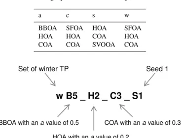
Table 1.Sets of target profiles used in the study.
a c s w
BBOA SFOA HOA SFOA
HOA HOA COA HOA
COA COA SVOOA COA
Set of winter TP Seed 1
w B5 _ H2 _ C3 _ S1
BBOA with an avalue of 0.5 COA with an avalue of 0.3
HOA with an avalue of 0.2
Figure 1.Coding used to identify the different runs.
wherep is the number of factors chosen,n the number of samples andmthe mass spectra. Ideally, if the model accu-rately captured the variability of the measured data, it would be expected to have a value ofQ / Qexp=1, but this value depends on fluctuations in the source profiles, over- or un-derestimation of input data errors and the model error.
Solutions using a least squares approach to solve a fac-tor analysis problem may have linear transformations, also known as rotations (Paatero and Hopke, 2009). One advan-tage of ME2 over PMF is that the rotational ambiguity can be reduced by using previous knowledge of profiles (for exam-ple mass spectra) or time series of different pollutants using the a value approach. Equation 4 was applied using differ-ent target profiles (TPs) (gi)and a range ofa values (a)to
constrain OA sources in different runs (gi,run).
gi,run=gi±a×gi (4)
Theavalue is a parameter that represents the degree of vari-ability of the target profile, which typically ranges from zero to one. The closer to zero, the more constrained the solution is (Lanz et al., 2008). The user should keep in mind that par-tially constrained solutions are carried out by compromising theQ / Qexpvalue, which should be monitored to determine the feasibility of the solutions.
2.2.1 Target profiles and levels of constraint
In this study, solutions obtained with ME-2 were constrained using the a value approach, by using four different sets of mass spectra from previous studies of TPs (Table 1). Set a of the TPs represents BBOA and HOA average factor profiles obtained from an analysis carried out on different mass spec-tra from a variety of monitoring sites across Europe (Crippa et al., 2014) and COA obtained from a study in Paris (Crippa et al., 2013a). Sets c, s and w were provided by Young et
al. (2015a) from a PMF analysis carried out on AMS mea-surements at the North Kensington site in London, 2012. The c TPs were obtained from an analysis performed on annual OA measured with a cToF-AMS (11 January 2012–23 Jan-uary 2013). Sets s and w were obtained from summer and winter measurements and taken with an HR-AMS (January– February and July–August 2012, respectively). The ACSM was specifically designed to deliver mass spectra that were equivalent to the AMS. With the AMS having a higher signal to noise ratio, it is expected that the use of its mass spectra as TPs is appropriate. Moreover, we consider AMS-generated TPs to be convenient to use, especially considering there are more of these available, including the ones obtained from the same site. In this study, the suitability of different TPs will be systematically assessed in the determination of OA sources using a wide range ofavalues.
A wide range of combinations of TP anda values were used during this analysis, all of them being run with three random initial values (seeds) to determine the stability of the solutions. Constraints were applied using one, two and three TPs; in all the solutions, there were at least two un-constrained factors. Figure 1 shows the coding used to iden-tify the different solutions, for example when constraining 3-factor profiles, e.g. wB5_H2_C3_S1.
2.3 Strategy to explore the solution space
The success of ME-2 relies on the additional use of a pri-ori information in the form of constraints. However, without a well-defined strategy or a limited analysis of the solution space, it may lead to a subjectively and inaccurately selected solution. Moreover, when possible, TPs from different stud-ies should be tested in order to determine which set of TPs are the most appropriate. Therefore, the following sections show the results of the analysis carried out on the data set of March–December 2013, to which the considerations pro-vided by Crippa et al. (2014) were applied. Moreover, new analysis techniques were developed to explore the solution space.
statistical tests applied, will be the one with values closest to one.
Trilinear regression is a new technique which is used to ex-plore the solution space in ME-2 analysis. Multilinear regres-sion has been previously applied to analyse the relationship between POA and combustion tracers (Allan et al., 2010; Liu et al., 2011; Young et al., 2015b) as well as polycyclic aro-matic hydrocarbons (Elser et al., 2016). This is used instead of simple linear regression because many of the combustion related variables will have multiple sources, such as biomass burning and traffic. Equation (3) shows the trilinear regres-sion equation used to analyse the relationship between POA and combustion tracers.
Y =A+B[BBOA]+C[HOA]+D[COA], (5) whereY is NOx, BC, or CO.
B,C andD slopes represent the contribution of BBOA, HOA and COA toY and the interceptAis representative of the Y background concentration. The following considera-tions should be taken into account: the slopes and intercepts should be positive as they represent air pollutant concentra-tions and the slopeDis used as a validation parameter, which should be close to zero due to its low contribution to BC, NOxand CO, owing to the fact that most cooking in the UK
uses electricity or natural gas as a source of heat (DECC, 2016; DEFRA, 2016). A non-zero value would indicate cor-relation with combustion tracers and thus the possibility that it is receiving interference from HOA, which has a similar mass spectrum. Chi square is used as a “goodness of fit” for which the lower the value, the better the fit between the anal-ysed pollutants.
3 Results
3.1 Exploring the solution space for March–December data set
This section shows the results from the analysis applied to determine the solution that best represents the OA sources for the complete data set March–December 2013, according to the statistical tests applied, when a total of eight uncon-strained and 25 conuncon-strained solutions were analysed.
3.1.1 Solutions,avalues and stability
Unconstrained runs withf peak=0 and three different seeds
were performed in order to determine the number of OA sources. Five was (BBOA, HOA, COA, SVOOA, LVOOA) the optimal number of sources (Fig. S1b in the Supplement), as it was possible to split the SOA into SVOOA and LVOOA. Further unconstrained analysis was performed by running 5-factor solutions with different f peaks, from−1 to 1 with steps of 0.1 (Fig. S4) in order to select the PMF solution to be compared with the ME-2 analysis. ME-2 is run using a
range ofa values, which were selected after trial and error and according to the literature (Lanz et al., 2008; Crippa et al., 2014; Petit et al., 2014), which suggests thata values depend on the similarity of the TP and the factor profile be-ing analysed. HOA mass spectra do not show high variability when compared to different sites, thus it is possible to restrict the constraint witha values of 0.1–0.2. On the other hand, COA and BBOA mass spectra from different sites show high variability and a looser constraint should be applied (for ex-ample,avalues 0.3–0.5 or higher).
Constraining only 1 or 2 factors of the 5-factor solutions gave the least favourable results with high residuals and mixing factor profiles. When analysing the different seeds, these solutions also showed high variability between seeds. Greater stability was found when 3 of the 5 factor solutions were constrained (Fig. S2), as also observed by Crippa et al. (2014). As a result, in this analysis, 5-factor solutions con-straining 3 factors will be analysed for the first seed. One PMF solution and two solutions constraining 2 factors were also used during the exploration (Fig. 2) for three sets of TPs.
3.1.2 Q / Qexp, diurnal residual and trilinear
regression
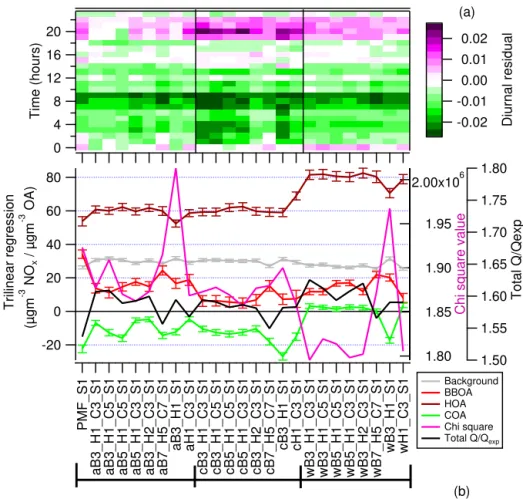
As an ideal solution, aQ / Qexp value of 1.0 would be ex-pected. However, there is not a standard criterion to define a satisfactoryQ / Qexpvalue, as a certain amount of model error will cause it to be systematically higher than unity (Ul-brich et al., 2009). When comparing different solutions from the same data set (Fig. 2b), it is possible to observe that there is not a significant variation on theQ / Qexp (ranging be-tween 1.88–2.2) when using differenta values, suggesting that all the solutions are mathematically acceptable. The un-constrained solution is the one with the lowest totalQ / Qexp with a value of 1.88, which is expected, as PMF calculates the solution by minimizing this value; however, the PMF solution has a high chi square and negative slope for COA (Fig. 2a), implying that this solution is not environmentally acceptable, thus it is necessary to analyse all the different parameters in Fig. 2 in order to select the solution that best identifies the OA sources.
Figure 2a shows the diurnal residual analysis in which so-lutions constrained with c TPs present a high positive resid-ual around 14:00–19:00 h. Solutions constrained with w TPs have a negative residual during early morning with a positive residual at 21:00 h. Hence, the solution with a better diurnal residual is within the solutions constrained with a TPs.
Figure 2b shows the trilinear regression outputs between NOx and POA for the different solutions (see Supplement
Sect. S3 for BC and CO trilinear regressions). All the solu-tions properly identified the background NOxconcentrations
out-80
60
40
20
0
-20
Trilinear regression
(µgm
-3 NO
x
/ µgm
-3 OA)
PMF_S1
aB3_H1_C3_S1 aB3_H1_C5_S1 aB5_H1_C5_S1 aB5_H1_C3_S1 aB3_H2_C3_S1 aB7_H5_C7_S1 aB3_H1_S1 aH1_C3_S1
cB3_H1_C3_S1 cB3_H1_C5_S1 cB5_H1_C5_S1 cB5_H1_C3_S1 cB3_H2_C3_S1 cB7_H5_C7_S1 cB3_H1_S1 cH1_C3_S1
wB3_H1_C3_S1 wB3_H1_C5_S1 wB5_H1_C5_S1 wB5_H1_C3_S1 wB3_H2_C3_S1 wB7_H5_C7_S1 wB3_H1_S1 wH1_C3_S1
2.00x10⁶
1.95
1.90
1.85
1.80
Chi square value
1.80
1.75
1.70
1.65
1.60
1.55
1.50
Total Q/Qexp
20
16
12
8
4
0
Time (hours)
0.02 0.01 0.00 -0.01 -0.02 Diurnal residual
(a)
(b) Background BBOA HOA COA Chi square Total Q/Qexp
Figure 2. (a)Diurnal residual,yaxis represents time up to 24 h andxaxis represents the different solutions with a variety of target profiles andavalues.(b)NOxtrilinear regression for solutions with different target profiles. BBOA represents the slope of µg m−3of NOx per
µg m−3of BBOA. The same applies for HOA and COA. Whiskers represent the 95 % confidence interval.
come of the diurnal residual analysis that the best solution, according to the statistical tests applied, is with the solutions constrained with a TPs. Additionally, trilinear regression out-puts show variations between different solutions constrained with a TPs with changes mainly in the chi square and the BBOA.
3.1.3 Diurnal concentrations and mass spectra
OA sources have characteristic diurnal trends, and they may be used, together with their respective mass spectra, to anal-yse the solutions and determine whether all the factors in the solution are environmentally suitable. BBOA showed low concentrations during the day and high concentrations at night, mainly related to domestic heating (Alfarra et al., 2007). HOA presents two peaks during the day related to commuting, one in the morning and another in the evening (Zhang et al., 2005). COA has two peaks related to OA emis-sions from cooking activities, one peak at noon and one peak in the evening (Allan et al., 2010). SVOOA is temperature dependent with low concentrations during the day, which in-crease in the evening due to the condensation of gas phase
pollutants. LVOOA, due to its regional origin, does not show high variations in its diurnal trend.
Diurnal concentrations for all the solutions (Supplement Sect. S3) were analysed to determine the main sources. Here, it was possible to observe that solutions with undesirable out-puts in the residual, totalQ / Qexpand/or trilinear regression were likely to have mixed diurnal concentrations between two sources. For example, in the case of c TP solutions, CO and BC trilinear regressions (Fig. S5a and b) show better COA slopes with values close to zero; however, due to the high diurnal residual (Fig. 2a) and HOA, with high concen-trations during the evening (Fig. S5c) suggesting mixing with BBOA, c TP solutions are not considered acceptable.
and 73 and a peak atm/z60 for COA, implying mixing with BBOA.
Finally, from this analysis, aB3_H2_C3_S1 was deter-mined to be the solution that best represents the OA sources for the March–December analysis, according to the statistical tests applied.
3.2 Seasonal analysis
When applying source apportionment, ME-2 considers that both TPs and factor profiles remain constant over time, which may not be the case for long periods of time in which mete-orological conditions and pollutant emissions related to hu-man activities vary greatly (Canonaco et al., 2015; Ripoll et al., 2015). Thus, the same analysis that was carried out on the March–December data set was applied to data divided into seasons of the year: spring (March, April and May), sum-mer (June, July and August) and autumn (September, Octo-ber and NovemOcto-ber); see Supplement Sect. S.3 for detailed information of the seasonal analysis.
From analysing the spring data set (Fig. S7), solutions constrained with a and c TPs were found to present the least favourable results with high chi-square values and neg-ative COA ratios in the trilinear analysis, as well as a higher negative diurnal residual. The solution wB3_H1_C3_S1 was deemed to be the best solution for the spring analysis. Solu-tions constrained with s and c TPs were the least favourable results for the summer analysis (Fig. S9), with low chi-square values in s target profiles, which show high negative residuals in the morning and at night. Since c TPs show a high positive residual around 15:00–18:00 h, the solution aB5_H1_C3_S1 was found to be the best solution for the summer analy-sis. In the autumn analysis (Fig. S11), solutions constrained with a and w TPs were found to be the least favourable re-sults, with high positive residuals in the morning and a target profiles also showing high chi-square values. The solution cB3_H1_S1 was deemed the best solution for the autumn analysis according to the statistical tests applied. It is worth mentioning that all plausible solutions deconvolved a high percentage of the total OA mass (Fig. S12), with summer be-ing the period with less OA mass estimated (90 %) and the other periods with more than 95 % of mass estimated from the total OA concentrations.
4 Discussion and atmospheric implications 4.1 Annual and seasonal solutions
In the following subsections, the outputs of annual and sea-sonal solutions are compared in order to further explore the variability of the different OA sources.
4.1.1 TotalQ / Qexpand diurnal residual
Having analysed the totalQ / Qexp, all the solutions obtained were mathematically acceptable and had small variations be-tween their different values: 1.95 for March–December, 2.01 for spring, 1.95 for summer and 1.96 for autumn (Fig. 3a).
Q / Qexpvalues obtained in this study are compared to val-ues obtained in different ME-2 studies. For example, Petit et al. (2014), in a study using an ACSM, obtained aQ / Qexp value of 6, while studies carried out in Spain during winter and summer obtained 1.15 and 0.38 respectively (Minguil-lón et al., 2015b).Q / Qexp values obtained with PMF are also comparable with values obtained in this study, for ex-ample Young et al. (2015a) obtained a value of 1.35 from an-nual measurements carried out with a cToF-AMS at this site. Allan et al. (2010) obtained differentQ / Qexpvalues for the analysis carried out on three different data sets: a value of 3.9 from measurements obtained using a HR-ToF-AMS and val-ues of 10.5 and 16.7 using a cToF-AMS. Crippa et al. (2013b) also identified aQ / Qexpvalue of 4.59 from HR-ToF-AMS measurements during July 2009 at the urban background site in Paris. Due to all this variability ofQ / Qexpvalues found in the literature, this parameter alone cannot be used as a cri-terion to determine the solution that best identifies the OA sources.
It is in the diurnal residual where we can observe a high variation (Fig. 3b), with autumn proving to be the most overestimated with negative residuals of −0.033 µg m−3, mainly in the morning and at night. On the other hand, sum-mer appears to be the most underestimated solution with values of 0.018 µg m−3, particularly between midday and 17:00 UTC. The fact that summer is underestimated from 12:00 to 17:00 UTC is probably related to the increase on photochemical activity, a situation that ME-2 is not able to capture as the mass spectra remains constant over the period analysed. It is important to notice that these diurnal resid-uals of 0.03 µg m−3or less are low compared with diurnal concentrations of the OA sources, which were in the range 0.1–0.6 µg m−3.
4.1.2 Trilinear regression analysis
80
60
40
20
0
Trilinear regression
(µgm
-3 NO
x
/ µgm
-3 OA)
March_Dec
Spring
Summer Autumn 2.2
2.1
2.0
1.9
1.8
Tot Q/Qexp
20
16
12
8
4
0
Time (hours)
March_Dec
Spring
Summer Autumn Bground
BBOA HOA COA Tot Q/Qexp
-30x10-3 -20 -10 0 10 20
Diurnal residual
(a) (b)
Figure 3.NOxtrilinear regression(a)and diurnal residual(b)for the different analyses.
The analysis presented in Sect. 4 shows that seasonal anal-ysis more accurately deconvolves OA sources, being able to obtain more detailed information that will be lost when run-ning ME-2 for long periods of time.
4.1.3 Target profiles (TPs) and their impact on the solutions
As previously mentioned, the chosen solutions were aB3_H2_C3_S1 for March–December, wB3_H1_C3_S1 for spring, aB5_H1_C3_S1 for summer and wB3_H1_S1 for au-tumn. The fact that the March–December and summer solu-tions were obtained with TP a is possibly due to the fact that these TPs represent an average from different mass spectra, becoming robust TPs which are able to deal with the vari-ations of the two data sets. There was one large data set (March–December) and one data set with concentrations af-fected by the different photochemical processes due to the high temperatures (summer). On the other hand, spring and autumn do not show these variations and their OA sources may be apportioned using winter TPs which were obtained under similar temperatures.
Looking at the c and s TPs, these were the ones with the least favourable results of all analyses carried out. This may be attributed to c being the only TP obtained with a cToF-AMS while the rest were obtained using a HR-cToF-AMS. In the case of TP s, the unfavourable outputs are again related to the high variability present during this period of time. This analysis shows the importance of using the appropriate TP when doing source apportionment as well as exploring so-lutions with different types of TPs in order to determine the OA sources.
4.2 Variability of factor profiles
The variability of the different solutions previously obtained may be explored further with the triangle plotsf44 vs.f43 (Ng et al., 2010; Morgan et al., 2010) andf44 vs.f60 (Cu-bison et al., 2011). The parametersf43,f44 andf60 rep-resent the ratio of the integrated signal at m/z43, 44 and 60, respectively, to the total signal in the organic compo-nent mass spectrum. Figure 4a shows that LVOOA, while having different values between solutions, is found in dis-tinct areas of the plot (connecting lines are used to make the SVOOA variability clearer), whereas SVOOA shows values of f44 vs. f43 with high variability. This analysis shows that the factors derived for SOA do not always conform to the model of LVOOA and SVOOA proposed by Jimenez et al. (2009). Furthermore, the fact that the lines are going in different directions to the seasons of year means that the factorization is identifying different aspects of the chemical complexity, as LVOOA and SVOOA (rather than originat-ing from primary emissions) are part of continuous physico-chemical processes involving gases, aerosols and meteoro-logical parameters among others. This serves to highlight that a 2-component model (LVOOA and SVOOA) is an over-simplification of a complex chemical system as concluded by Canonaco et al. (2015), who found significantf44 vs.f43 differences for summer and winter analyses.
0.35
0.30
0.25
0.20
0.15
0.10
0.05
0.00
f44
50x10-3 40
30 20 10 0
f60 0.35
0.30
0.25
0.20
0.15
0.10
0.05
0.00
f44
0.20 0.15 0.10 0.05 0.00
f43
BBOA HOA COA SVOOA LVOOA
Spring Summer
Autumn March–Dec
(a) SVOOA (b)
LVOOA
Spring Summer
Autumn March–Dec
Figure 4. (a)f44 vs.f43 and(b)f44 vs.f60 plots for different periods of time.
two types of solid fuel OA factors, attributed to differences in burning efficiency. BBOA evolution has been frequently observed with highf44 and lowf60 values due to ageing, oxidation and cloud processing (Huffman et al., 2009; Cubi-son et al., 2011). Thus, it was possible to obtain a variety of BBOA for the different seasons of the year, ranging from a fresh BBOA with a highf60 during autumn to a more oxi-dized BBOA with a lowf60 during summer.
For all the solutions, COA presents anf60 value of ap-proximately 0.01, which has been previously identified by Mohr et al. (2009), who obtainedf60 values of 0.015–0.03 for different types of meat cooking. The fact that all the COA mass spectra present similarf44 :f60 ratios suggests that the COA footprint is relatively constant over the differ-ent seasons and, along with HOA, it is the more appropriate source to constrain when applying theavalue approach.
4.3 Petrol and diesel contribution to traffic emissions
Traffic emissions contribute significantly to air pollution (Beevers et al., 2012; Carslaw et al., 2013; May et al., 2014). In order to better analyse traffic emissions and their impact on air quality, it is necessary to understand the fuel type and pollutant contribution from different vehicles. In particular, the United Kingdom has a considerable percentage of diesel-fuelled vehicles; according to the vehicle licensing statistics, the percentage of diesel-fuelled vehicles licensed has been increasing over the last few years from 22 in 2006 to 36.2 % in 2014 while petrol-fuelled vehicles decreased from 77.7 to 62.9 % (GOV.UK, 2015).
Diesel emits higher NOx and HOA concentrations
com-pared to petrol, while petrol emits higher concentrations of CO, according to the National Atmospheric Emissions in-ventory (DEFRA, 2016), during 2014 the emission factors (units in kilotonnes of pollutant per megatonne of fuel used) were 11–12 for diesel and 1.9–4.3 for petrol in the case of NOxand 2.4–5.6 for diesel and 11–50 for petrol in the case
of CO. Moreover, there are variations between light-duty
1.6
1.4
1.2
1.0
0.8
0.6
0.4
WD/WE ratios
March_Dec Spring Summer Autumn NOx/HOA
CO/HOA NOx/∆CO
Figure 5.WD/WE ratios to analyse petrol and diesel contribu-tions.
diesel (LDD) and heavy-duty diesel (HDD) emissions (GLA, 2013), with LDD emitting higher NOx concentrations and
HDD emitting higher HOA concentrations.
It is possible to qualitatively analyse the impact of differ-ent fuels on air pollution by looking at weekday/weekend ratios (WD/WE), as previously done in several studies (Bahreini et al., 2012; Tao and Harley, 2014; DeWitt et al., 2015) and stating the hypothesis that different fuels will have different pollutant contributions during the week. This analy-sis considers WD as Monday to Friday and WE as only Sun-day to eliminate the mixed traffic on SaturSun-day. Another con-sideration is that the heavy-duty/light-duty emissions fleet ra-tio is higher during the week (Lough et al., 2006; Bahreini et al., 2012; Heo et al., 2015). It is also important to state that heavy-duty vehicles are exclusively diesel fuelled whereas light-duty vehicles are fuelled with a mixture of diesel and petrol.
(Sun-60
40
20
0
PM
2.5
(
µ
g·m
-3 )
01/05/2013 01/07/2013 01/09/2013 01/11/2013
Date 100
80
60
40
20
0
PM
1
composition (%)
BBOA HOA COA BC SVOOA LVOOA NO3
NH4
SO4 (a)
(b)
High
moderate
Primary
Secondary
5 % 4 % 8 % 23 %
5 %
20 %
17 % 8 %
10 %
(c)
Figure 6. (a)Daily PM2.5concentrations,(b)daily and(c)total PM1composition, purple line in Fig. 6c separates secondary and primary aerosols.
day) to analyse the WD/WE contributions. Subsequently, it was possible to determine WD/WE ratios for the slopes NOx/HOA and CO/HOA.
In order to compare these trilinear outputs with the WD/WE ratios between NOxand CO, NOx/ 1CO was
cal-culated from average concentrations. There is a difference in lifetime between CO (lifetime of months) and NOx(lifetime
of hours), thus it is important to consider the background CO concentrations to be able to compare NOxand CO
concentra-tions. It is necessary to perform a linear regression between CO and NOx and calculate1CO, which is the average CO
concentration minus the intercept from the CO : NOx linear
regression.
Figure 5 shows the WD/WE ratios, from which it is pos-sible to observe NOx/ 1CO ratios of 1.25, 1.35 and 1.36 for
March–December, summer and autumn, respectively, sug-gesting diesel has a higher contribution during WD compared to petrol. These findings are confirmed by the CO/HOA ratios, which, for the same periods of time, are lower than one (0.8, 0.45 and 0.9), suggesting a lower contribution of petrol during weekdays compared to diesel. In spring, there are no considerable changes to the WD/WE ratios, although a higher contribution of petrol is shown during WD with values of 1.28 for CO/HOA and low diesel contribution. Analysing the NOx/HOA ratios, the seasonal ratios show
values of 1.07, 1.06 and 1.05 suggesting a slightly higher contribution of LDD during WD than HDD.
4.4 PM2.5daily concentrations and PM1composition
PM2.5has been widely studied due to its potential to cause negative effects on health (Pope and Dockery, 2006; Harri-son et al., 2012; Bohnenstengel et al., 2014). This adverse impact is directly connected to the size of the particles, mak-ing PM1more detrimental to health than PM2.5(Ramgolam et al., 2009). Moreover, analysing the aerosol contribution to PM1and its association with PM2.5concentrations allows the possible influence of PM1on PM2.5 levels to be deter-mined. According to the Daily Air Quality Index (DAQI), PM2.5 concentrations are considered moderate when daily concentrations are between 35 and 52 µg m−3and high when levels are between 53 and 69 µg m−3. Daily PM
2.5 concen-trations during the sampling period show that the majority of daily concentrations were considered to be low episodes (Fig. 6a), with 10 episodes of moderate concentrations and only two episodes of high PM2.5 concentrations (55.2 and 61.5 µg m−3).
iden-tified. In the episode in March, high BBOA concentrations were observed, whereas during the episodes in April and September, higher concentrations of LVOOA were detected. Defining BBOA, HOA COA and BC as primary and SVOOA, LVOOA, NO3, NH4 and SO4 as secondary aerosols, the main PM1 contributors to PM2.5 concentra-tions are secondary aerosols with a total contribution of 61 % (Fig. 6c). These findings agree with a previous study at this same monitoring site carried out by Young et al. (2015a), who found secondary aerosols to be the predominant source of PM1over the year, with different secondary inorganic and organic aerosol contributions between winter and summer.
5 Conclusions
This study presents the source apportionment carried out us-ing ME-2 within SoFi 4.8 of OA concentrations, measured with an ACSM from March to December 2013 at the urban background site in North Kensington, London; the first time it was deployed in the UK.
ME-2 proved to be a robust tool to deconvolve OA sources. This study highlighted the importance of using appropri-ate mass spectra as target profiles and a values when ex-ploring the solution space. With the implementation of new techniques to compare different solutions, it was possible to systematically determine the solution with the best sep-aration of OA sources, mathematically and environmentally speaking. The comparison carried out between the solution for the March–December data set and the seasonal solutions showed high variations mainly in the SVOOA and the BBOA sources, with wide range of f44 :f43 values for SVOOA (Fig. 4a) andf60 values ranging from 13×10−3for summer
to 24×10−3for autumn (Fig. 4b). These variations support the importance of running ME-2 when weather conditions and emissions from human activities are less variable, such as seasonal analyses.
SVOOA presented a high variability in the oxidation state during the different seasons. This is due to the nature of SVOOA being affected mainly by high temperatures and ME-2 not being able to completely determine SVOOA con-centrations. These results support the indication that is not an accurate practice to use SVOOA as a target profile when analysing solutions. Trilinear regressions deliver quantitative information about the ratios between combustion tracers and POA. These ratios may be used as a proxy for other urban background sites to estimate POA concentrations.
From analysing heavy- and light-duty diesel emissions, the main contributor on weekdays was found to be from diesel emissions, particularly LDD emissions. Thus, in order to re-duce traffic emissions on weekdays, LDD vehicles should be targeted. For the PM2.5 analysis (March–December 2013), the main PM1contributors to these concentrations were sec-ondary aerosols and BC, which means that PM1contributors to PM2.5concentrations are related to emissions from
com-bustion activities and secondary pollutants produced in the atmosphere.
This study delivers mass spectra and time series of OA sources for a long-term period as well as seasons of the year, and may be used in future ME-2 studies as TPs. Further-more, the scientific findings provide significant information to strengthen legislation as well as to support health studies that aim to improve air quality in the UK.
6 Data availability
ACSM data used in this paper have been archived at http://browse.ceda.ac.uk/browse/badc/clearflo/data/ long-term. Other monitoring data are available at https://uk-air.defra.gov.uk/data/data_selector.
The Supplement related to this article is available online at doi:10.5194/acp-16-15545-2016-supplement.
Author contributions. David C. Green, Ernesto Reyes-Villegas and James D. Allan designed the project; David C. Green and Max Priestman operated, calibrated and performed QA of ACSM data; Ernesto Reyes-Villegas performed the data analy-sis; Ernesto Reyes-Villegas, Francesco Canonaco, David C. Green, Hugh Coe, André S. H. Prévôt, and James D. Allan wrote the paper.
Acknowledgements. Ernesto Reyes-Villegas is supported by a
studentship by the National Council of Science and Technology– Mexico (CONACYT) under registry number 217687.
Edited by: L. M. Russell
Reviewed by: four anonymous referees
References
Alfarra, M. R., Prevot, A. S. H., Szidat, S., Sandradewi, J., Weimer, S., Lanz, V. A., Schreiber, D., Mohr, M., and Baltensperger, U.: Identification of the mass spectral signature of organic aerosols from wood burning emissions, Environ. Sci. Technol., 41, 5770– 5777, doi:10.1021/Es062289b, 2007.
Allan, J. D., Delia, A. E., Coe, H., Bower, K. N., Alfarra, M. R., Jimenez, J. L., Middlebrook, A. M., Drewnick, F., Onasch, T. B., Canagaratna, M. R., Jayne, J. T., and Worsnop, D. R.: A generalised method for the extraction of chemically resolved mass spectra from aerodyne aerosol mass spectrometer data, J. Aerosol. Sci., 35, 909–922, doi:10.1016/j.jaerosci.2004.02.007, 2004.
Bahreini, R., Middlebrook, A. M., de Gouw, J. A., Warneke, C., Trainer, M., Brock, C. A., Stark, H., Brown, S. S., Dube, W. P., Gilman, J. B., Hall, K., Holloway, J. S., Kuster, W. C., Perring, A. E., Prevot, A. S. H., Schwarz, J. P., Spackman, J. R., Szi-dat, S., Wagner, N. L., Weber, R. J., Zotter, P., and Parrish, D. D.: Gasoline emissions dominate over diesel in formation of sec-ondary organic aerosol mass, Geophys. Res. Lett., 39, L06805, doi:10.1029/2011gl050718, 2012.
Beccaceci, S., McGhee, E. A., Brown, R. J. C., and Green, D. C.: A comparison between a semi-continuous analyzer and filter-based method for measuring anion and cation concentrations in pm10 at an urban background site in london, Aerosol Sci. Technol., 49, 793–801, doi:10.1080/02786826.2015.1073848, 2015.
Beevers, S. D., Westmoreland, E., de Jong, M. C., Williams, M. L., and Carslaw, D. C.: Trends in NOx and NO2 emissions from road traffic in great britain, Atmos. Environ., 54, 107–116, doi:10.1016/j.atmosenv.2012.02.028, 2012.
Bigi, A. and Harrison, R. M.: Analysis of the air pollution climate at a central urban background site, Atmos. Environ., 44, 2004– 2012, doi:10.1016/j.atmosenv.2010.02.028, 2010.
Bohnenstengel, S. I., Belcher, S. E., Aiken, A., Allan, J. D., Allen, G., Bacak, A., Bannan, T. J., Barlow, J. F., Beddows, D. C. S., Bloss, W. J., Booth, A. M., Chemel, C., Coceal, O., Di Marco, C. F., Dubey, M. K., Faloon, K. H., Fleming, Z. L., Furger, M., Gietl, J. K., Graves, R. R., Green, D. C., Grimmond, C. S. B., Halios, C. H., Hamilton, J. F., Harrison, R. M., Heal, M. R., Heard, D. E., Helfter, C., Herndon, S. C., Holmes, R. E., Hop-kins, J. R., Jones, A. M., Kelly, F. J., Kotthaus, S., Langford, B., Lee, J. D., Leigh, R. J., Lewis, A. C., Lidster, R. T., Lopez-Hilfiker, F. D., McQuaid, J. B., Mohr, C., Monks, P. S., Nemitz, E., Ng, N. L., Percival, C. J., Prévôt, A. S. H., Ricketts, H. M. A., Sokhi, R., Stone, D., Thornton, J. A., Tremper, A. H., Valach, A. C., Visser, S., Whalley, L. K., Williams, L. R., Xu, L., Young, D. E., and Zotter, P.: Meteorology, air quality, and health in lon-don: The clearflo project, B. Am. Meteorol. Soc., 96, 779–804, doi:10.1175/bams-d-12-00245.1, 2014.
Bozzetti, C., Daellenbach, K. R., Hueglin, C., Fermo, P., Sciare, J., Kasper-Giebl, A., Mazar, Y., Abbaszade, G., El Kazzi, M., Gonzalez, R., Shuster-Meiseles, T., Flasch, M., Wolf, R., Kˇre-pelová, A., Canonaco, F., Schnelle-Kreis, J., Slowik, J. G., Zim-mermann, R., Rudich, Y., Baltensperger, U., El Haddad, I., and Prévôt, A. S. H.: Size-resolved identification, characteriza-tion, and quantification of primary biological organic aerosol at a european rural site, Environ. Sci. Technol., 50, 3425–3434, doi:10.1021/acs.est.5b05960, 2016.
Bruns, E. A., El Haddad, I., Keller, A., Klein, F., Kumar, N. K., Pieber, S. M., Corbin, J. C., Slowik, J. G., Brune, W. H., Bal-tensperger, U., and Prévôt, A. S. H.: Inter-comparison of lab-oratory smog chamber and flow reactor systems on organic aerosol yield and composition, Atmos. Meas. Tech., 8, 2315– 2332, doi:10.5194/amt-8-2315-2015, 2015.
Budisulistiorini, S. H., Canagaratna, M. R., Croteau, P. L., Bau-mann, K., Edgerton, E. S., Kollman, M. S., Ng, N. L., Verma, V., Shaw, S. L., Knipping, E. M., Worsnop, D. R., Jayne, J. T., Weber, R. J., and Surratt, J. D.: Intercomparison of an Aerosol Chemical Speciation Monitor (ACSM) with ambient fine aerosol measurements in downtown Atlanta, Georgia, Atmos. Meas. Tech., 7, 1929–1941, doi:10.5194/amt-7-1929-2014, 2014.
Canonaco, F., Crippa, M., Slowik, J. G., Baltensperger, U., and Prévôt, A. S. H.: SoFi, an IGOR-based interface for the efficient use of the generalized multilinear engine (ME-2) for the source apportionment: ME-2 application to aerosol mass spectrome-ter data, Atmos. Meas. Tech., 6, 3649–3661, doi:10.5194/amt-6-3649-2013, 2013.
Canonaco, F., Slowik, J. G., Baltensperger, U., and Prévôt, A. S. H.: Seasonal differences in oxygenated organic aerosol compo-sition: implications for emissions sources and factor analysis, Atmos. Chem. Phys., 15, 6993–7002, doi:10.5194/acp-15-6993-2015, 2015.
Carslaw, D. C., Williams, M. L., Tate, J. E., and Beevers, S. D.: The importance of high vehicle power for passenger car emissions, Atmos. Environ., 68, 8–16, doi:10.1016/j.atmosenv.2012.11.033, 2013.
Crippa, M., DeCarlo, P. F., Slowik, J. G., Mohr, C., Heringa, M. F., Chirico, R., Poulain, L., Freutel, F., Sciare, J., Cozic, J., Di Marco, C. F., Elsasser, M., Nicolas, J. B., Marchand, N., Abidi, E., Wiedensohler, A., Drewnick, F., Schneider, J., Borrmann, S., Nemitz, E., Zimmermann, R., Jaffrezo, J.-L., Prévôt, A. S. H., and Baltensperger, U.: Wintertime aerosol chemical compo-sition and source apportionment of the organic fraction in the metropolitan area of Paris, Atmos. Chem. Phys., 13, 961–981, doi:10.5194/acp-13-961-2013, 2013a.
Crippa, M., El Haddad, I., Slowik, J. G., DeCarlo, P. F., Mohr, C., Heringa, M. F., Chirico, R., Marchand, N., Sciare, J., Bal-tensperger, U., and Prevot, A. S. H.: Identification of marine and continental aerosol sources in paris using high resolution aerosol mass spectrometry, J. Geophys. Res.-Atmos., 118, 1950–1963, doi:10.1002/Jgrd.50151, 2013b.
Crippa, M., Canonaco, F., Lanz, V. A., Äijälä, M., Allan, J. D., Car-bone, S., Capes, G., Ceburnis, D., Dall’Osto, M., Day, D. A., De-Carlo, P. F., Ehn, M., Eriksson, A., Freney, E., Hildebrandt Ruiz, L., Hillamo, R., Jimenez, J. L., Junninen, H., Kiendler-Scharr, A., Kortelainen, A.-M., Kulmala, M., Laaksonen, A., Mensah, A. A., Mohr, C., Nemitz, E., O’Dowd, C., Ovadnevaite, J., Pan-dis, S. N., Petäjä, T., Poulain, L., Saarikoski, S., Sellegri, K., Swietlicki, E., Tiitta, P., Worsnop, D. R., Baltensperger, U., and Prévôt, A. S. H.: Organic aerosol components derived from 25 AMS data sets across Europe using a consistent ME-2 based source apportionment approach, Atmos. Chem. Phys., 14, 6159– 6176, doi:10.5194/acp-14-6159-2014, 2014.
Cubison, M. J., Ortega, A. M., Hayes, P. L., Farmer, D. K., Day, D., Lechner, M. J., Brune, W. H., Apel, E., Diskin, G. S., Fisher, J. A., Fuelberg, H. E., Hecobian, A., Knapp, D. J., Mikoviny, T., Riemer, D., Sachse, G. W., Sessions, W., Weber, R. J., Wein-heimer, A. J., Wisthaler, A., and Jimenez, J. L.: Effects of aging on organic aerosol from open biomass burning smoke in aircraft and laboratory studies, Atmos. Chem. Phys., 11, 12049–12064, doi:10.5194/acp-11-12049-2011, 2011.
Dall’Osto, M., Thorpe, A., Beddows, D. C. S., Harrison, R. M., Barlow, J. F., Dunbar, T., Williams, P. I., and Coe, H.: Remark-able dynamics of nanoparticles in the urban atmosphere, At-mos. Chem. Phys., 11, 6623–6637, doi:10.5194/acp-11-6623-2011, 2011.
DEFRA: National atmospheric emissions inventory, http://naei. defra.gov.uk/data/, last access: 15 August 2016.
A., Besombes, J. L., Jaffrezo, J. L., Wortham, H., and Marc-hand, N.: Near-highway aerosol and gas-phase measurements in a high-diesel environment, Atmos. Chem. Phys., 15, 4373–4387, doi:10.5194/acp-15-4373-2015, 2015.
Digest of United Kingdom energy statistics 2015: https: //www.gov.uk/government/uploads/system/uploads/attachment_ data/file/450302/DUKES_2015.pdf(last access: 12 August 2016), 2015.
Elser, M., Huang, R.-J., Wolf, R., Slowik, J. G., Wang, Q., Canonaco, F., Li, G., Bozzetti, C., Daellenbach, K. R., Huang, Y., Zhang, R., Li, Z., Cao, J., Baltensperger, U., El-Haddad, I., and Prévôt, A. S. H.: New insights into PM2.5chemical composition and sources in two major cities in China during extreme haze events using aerosol mass spectrometry, Atmos. Chem. Phys., 16, 3207–3225, doi:10.5194/acp-16-3207-2016, 2016.
Fountoukis, C., Megaritis, A. G., Skyllakou, K., Charalampidis, P. E., Denier van der Gon, H. A. C., Crippa, M., Prévôt, A. S. H., Fachinger, F., Wiedensohler, A., Pilinis, C., and Pan-dis, S. N.: Simulating the formation of carbonaceous aerosol in a European Megacity (Paris) during the MEGAPOLI sum-mer and winter campaigns, Atmos. Chem. Phys., 16, 3727–3741, doi:10.5194/acp-16-3727-2016, 2016.
Fröhlich, R., Crenn, V., Setyan, A., Belis, C. A., Canonaco, F., Favez, O., Riffault, V., Slowik, J. G., Aas, W., Aijälä, M., Alastuey, A., Artiñano, B., Bonnaire, N., Bozzetti, C., Bressi, M., Carbone, C., Coz, E., Croteau, P. L., Cubison, M. J., Esser-Gietl, J. K., Green, D. C., Gros, V., Heikkinen, L., Herrmann, H., Jayne, J. T., Lunder, C. R., Minguillón, M. C., Mocnik, G., O’Dowd, C. D., Ovadnevaite, J., Petralia, E., Poulain, L., Priestman, M., Ripoll, A., Sarda-Estève, R., Wiedensohler, A., Baltensperger, U., Sciare, J., and Prévôt, A. S. H.: ACTRIS ACSM intercompar-ison – Part 2: Intercomparintercompar-ison of ME-2 organic source apportion-ment results from 15 individual, co-located aerosol mass spec-trometers, Atmos. Meas. Tech., 8, 2555–2576, doi:10.5194/amt-8-2555-2015, 2015.
GOV UK: Vehicles statistics, https://www.gov.uk/government/ collections/vehicles-statistics, last access: 4 August 2015. Harrison, R. M., Laxen, D., Moorcroft, S., and Laxen, K.:
Processes affecting concentrations of fine particulate matter (pm2.5) in the uk atmosphere, Atmos. Environ., 46, 115–124, doi:10.1016/j.atmosenv.2011.10.028, 2012.
Hennigan, C. J., Miracolo, M. A., Engelhart, G. J., May, A. A., Presto, A. A., Lee, T., Sullivan, A. P., McMeeking, G. R., Coe, H., Wold, C. E., Hao, W.-M., Gilman, J. B., Kuster, W. C., de Gouw, J., Schichtel, B. A., Collett Jr., J. L., Kreidenweis, S. M., and Robinson, A. L.: Chemical and physical transformations of organic aerosol from the photo-oxidation of open biomass burning emissions in an environmental chamber, Atmos. Chem. Phys., 11, 7669–7686, doi:10.5194/acp-11-7669-2011, 2011. Henry, R. C., Lewis, C. W., Hopke, P. K., and Williamson, H. J.:
Review of receptor model fundamentals, Atmos. Environ., 18, 1507–1515, doi:10.1016/0004-6981(84)90375-5, 1984. Heo, J., de Foy, B., Olson, M. R., Pakbin, P., Sioutas,
C., and Schauer, J. J.: Impact of regional transport on the anthropogenic and biogenic secondary organic aerosols in the los angeles basin, Atmos. Environ., 103, 171–179, doi:10.1016/j.atmosenv.2014.12.041, 2015.
Hildebrandt, L., Kostenidou, E., Lanz, V. A., Prevot, A. S. H., Bal-tensperger, U., Mihalopoulos, N., Laaksonen, A., Donahue, N.
M., and Pandis, S. N.: Sources and atmospheric processing of or-ganic aerosol in the Mediterranean: insights from aerosol mass spectrometer factor analysis, Atmos. Chem. Phys., 11, 12499– 12515, doi:10.5194/acp-11-12499-2011, 2011.
Huang, X.-F., He, L.-Y., Hu, M., Canagaratna, M. R., Sun, Y., Zhang, Q., Zhu, T., Xue, L., Zeng, L.-W., Liu, X.-G., Zhang, Y.-H., Jayne, J. T., Ng, N. L., and Worsnop, D. R.: Highly time-resolved chemical characterization of atmospheric submi-cron particles during 2008 Beijing Olympic Games using an Aerodyne High-Resolution Aerosol Mass Spectrometer, Atmos. Chem. Phys., 10, 8933–8945, doi:10.5194/acp-10-8933-2010, 2010.
Huffman, J. A., Docherty, K. S., Mohr, C., Cubison, M. J., Ul-brich, I. M., Ziemann, P. J., Onasch, T. B., and Jimenez, J. L.: Chemically-resolved volatility measurements of organic aerosol from different sources, Environ. Sci. Technol., 43, 5351–5357, doi:10.1021/es803539d, 2009.
Jimenez, J., Canagaratna, M., Donahue, N., Prevot, A., Zhang, Q., Kroll, J., DeCarlo, P., Allan, J., Coe, H., and Ng, N.: Evolution of organic aerosols in the atmosphere, Science, 326, 1525–1529, 2009.
Jones, A. M. and Harrison, R. M.: Interpretation of partic-ulate elemental and organic carbon concentrations at rural, urban and kerbside sites, Atmos. Environ., 39, 7114–7126, doi:10.1016/j.atmosenv.2005.08.017, 2005.
Jones, A. M., Harrison, R. M., and Baker, J.: The wind speed dependence of the concentrations of airborne par-ticulate matter and nox, Atmos. Environ., 44, 1682–1690, doi:10.1016/j.atmosenv.2010.01.007, 2010.
Keywood, M., Cope, M., Meyer, C. P. M., Iinuma, Y., and Emmer-son, K.: When smoke comes to town: The impact of biomass burning smoke on air quality, Atmos. Environ., 121, 13–21, doi:10.1016/j.atmosenv.2015.03.050, 2015.
Kupiainen, K. and Klimont, Z.: Primary emissions of fine car-bonaceous particles in europe, Atmos. Environ., 41, 2156–2170, doi:10.1016/j.atmosenv.2006.10.066, 2007.
Lanz, V. A., Alfarra, M. R., Baltensperger, U., Buchmann, B., Hueglin, C., and Prévôt, A. S. H.: Source apportionment of sub-micron organic aerosols at an urban site by factor analytical mod-elling of aerosol mass spectra, Atmos. Chem. Phys., 7, 1503– 1522, doi:10.5194/acp-7-1503-2007, 2007.
Lanz, V. A., Alfarra, M. R., Baltensperger, U., Buchmann, B., Hueglin, C., Szidat, S., Wehrli, M. N., Wacker, L., Weimer, S., Caseiro, A., Puxbaum, H., and Prevot, A. S. H.: Source attribu-tion of submicron organic aerosols during wintertime inversions by advanced factor analysis of aerosol mass spectra, Environ. Sci. Technol., 42, 214–220, doi:10.1021/Es0707207, 2008. Liu, D., Allan, J., Corris, B., Flynn, M., Andrews, E., Ogren, J.,
Beswick, K., Bower, K., Burgess, R., Choularton, T., Dorsey, J., Morgan, W., Williams, P. I., and Coe, H.: Carbonaceous aerosols contributed by traffic and solid fuel burning at a polluted rural site in Northwestern England, Atmos. Chem. Phys., 11, 1603–1619, doi:10.5194/acp-11-1603-2011, 2011.
Liu, Y. J. and Harrison, R. M.: Properties of coarse particles in the atmosphere of the united kingdom, Atmos. Environ., 45, 3267– 3276, doi:10.1016/j.atmosenv.2011.03.039, 2011.
GLA: London atmospheric emissions inven-tory 2013, http://data.london.gov.uk/dataset/ london-atmospheric-emissions-inventory-2013 (last access: 18 August 2016), 2013.
Lough, G. C., Schauer, J. J., and Lawson, D. R.: Day-of-week trends in carbonaceous aerosol composition in the urban atmosphere, Atmos. Environ., 40, 4137–4149, doi:10.1016/j.atmosenv.2006.03.009, 2006.
May, A. A., Nguyen, N. T., Presto, A. A., Gordon, T. D., Lipsky, E. M., Karve, M., Gutierrez, A., Robertson, W. H., Zhang, M., Brandow, C., Chang, O., Chen, S., Cicero-Fernandez, P., Dink-ins, L., Fuentes, M., Huang, S.-M., Ling, R., Long, J., Mad-dox, C., Massetti, J., McCauley, E., Miguel, A., Na, K., Ong, R., Pang, Y., Rieger, P., Sax, T., Truong, T., Vo, T., Chattopad-hyay, S., Maldonado, H., Maricq, M. M., and Robinson, A. L.: Gas- and particle-phase primary emissions from in-use, on-road gasoline and diesel vehicles, Atmos. Environ., 88, 247–260, doi:10.1016/j.atmosenv.2014.01.046, 2014.
Milic, A., Miljevic, B., Alroe, J., Mallet, M., Canonaco, F., Prevot, A. S. H., and Ristovski, Z. D.: The ambient aerosol characterization during the prescribed bushfire sea-son in brisbane 2013, Sci. Total Environ., 560–561, 225–232, doi:10.1016/j.scitotenv.2016.04.036, 2016.
Minguillón, M. C., Brines, M., Pérez, N., Reche, C., Pandolfi, M., Fonseca, A. S., Amato, F., Alastuey, A., Lyasota, A., Co-dina, B., Lee, H. K., Eun, H. R., Ahn, K. H., and Querol, X.: New particle formation at ground level and in the vertical col-umn over the barcelona area, Atmos. Res., 164–165, 118–130, doi:10.1016/j.atmosres.2015.05.003, 2015a.
Minguillón, M. C., Ripoll, A., Pérez, N., Prévôt, A. S. H., Canonaco, F., Querol, X., and Alastuey, A.: Chemical characteri-zation of submicron regional background aerosols in the western Mediterranean using an Aerosol Chemical Speciation Monitor, Atmos. Chem. Phys., 15, 6379–6391, doi:10.5194/acp-15-6379-2015, 2015b.
Mohr, C., Huffman, J. A., Cubison, M. J., Aiken, A. C., Docherty, K. S., Kimmel, J. R., Ulbrich, I. M., Hannigan, M., and Jimenez, J. L.: Characterization of primary organic aerosol emissions from meat cooking, trash burning, and motor vehicles with high-resolution aerosol mass spectrometry and comparison with ambi-ent and chamber observations, Environ. Sci. Technol., 43, 2443– 2449, doi:10.1021/Es8011518, 2009.
Mohr, C., DeCarlo, P. F., Heringa, M. F., Chirico, R., Slowik, J. G., Richter, R., Reche, C., Alastuey, A., Querol, X., Seco, R., Peñuelas, J., Jiménez, J. L., Crippa, M., Zimmermann, R., Bal-tensperger, U., and Prévôt, A. S. H.: Identification and quan-tification of organic aerosol from cooking and other sources in Barcelona using aerosol mass spectrometer data, Atmos. Chem. Phys., 12, 1649–1665, doi:10.5194/acp-12-1649-2012, 2012. Morgan, W. T., Allan, J. D., Bower, K. N., Highwood, E. J., Liu,
D., McMeeking, G. R., Northway, M. J., Williams, P. I., Krejci, R., and Coe, H.: Airborne measurements of the spatial distribu-tion of aerosol chemical composidistribu-tion across Europe and evolu-tion of the organic fracevolu-tion, Atmos. Chem. Phys., 10, 4065–4083, doi:10.5194/acp-10-4065-2010, 2010.
Ng, N. L., Canagaratna, M. R., Zhang, Q., Jimenez, J. L., Tian, J., Ulbrich, I. M., Kroll, J. H., Docherty, K. S., Chhabra, P. S., Bahreini, R., Murphy, S. M., Seinfeld, J. H., Hildebrandt, L., Donahue, N. M., DeCarlo, P. F., Lanz, V. A., Prévôt, A. S. H., Dinar, E., Rudich, Y., and Worsnop, D. R.: Organic aerosol components observed in Northern Hemispheric datasets from Aerosol Mass Spectrometry, Atmos. Chem. Phys., 10, 4625– 4641, doi:10.5194/acp-10-4625-2010, 2010.
Ng, N. L., Herndon, S. C., Trimborn, A., Canagaratna, M. R., Croteau, P., Onasch, T. B., Sueper, D., Worsnop, D. R., Zhang, Q., and Sun, Y.: An aerosol chemical speciation monitor (acsm) for routine monitoring of the composition and mass concentra-tions of ambient aerosol, Aerosol Sci. Technol., 45, 780–794, 2011.
Ortega, A. M., Day, D. A., Cubison, M. J., Brune, W. H., Bon, D., de Gouw, J. A., and Jimenez, J. L.: Secondary organic aerosol formation and primary organic aerosol oxidation from biomass-burning smoke in a flow reactor during FLAME-3, Atmos. Chem. Phys., 13, 11551–11571, doi:10.5194/acp-13-11551-2013, 2013.
Paatero, P. and Tapper, U.: Positive matrix factorization: A non-negative factor model with optimal utilization of error estimates of data values, Environmetrics, 5, 111–126, 1994.
Paatero, P.: The multilinear engine: A table-driven, least squares program for solving multilinear problems, including the n-way parallel factor analysis model, J. Comput. Graph. Stat., 8, 854– 888, doi:10.2307/1390831, 1999.
Paatero, P. and Hopke, P. K.: Rotational tools for factor analytic models, J. Chemom., 23, 91–100, 2009.
Paatero, P., Hopke, P. K., Song, X. H., and Ramadan, Z.: Un-derstanding and controlling rotations in factor analytic mod-els, Chemometr. Intell. Lab., 60, 253–264, doi:10.1016/S0169-7439(01)00200-3, 2002.
Petit, J.-E., Favez, O., Sciare, J., Canonaco, F., Croteau, P., Moc-nik, G., Jayne, J., Worsnop, D., and Leoz-Garziandia, E.: Sub-micron aerosol source apportionment of wintertime pollution in Paris, France by double positive matrix factorization (PMF2) us-ing an aerosol chemical speciation monitor (ACSM) and a multi-wavelength Aethalometer, Atmos. Chem. Phys., 14, 13773– 13787, doi:10.5194/acp-14-13773-2014, 2014.
Petit, J.-E., Favez, O., Sciare, J., Crenn, V., Sarda-Estève, R., Bon-naire, N., Mocnik, G., Dupont, J.-C., Haeffelin, M., and Leoz-Garziandia, E.: Two years of near real-time chemical compo-sition of submicron aerosols in the region of Paris using an Aerosol Chemical Speciation Monitor (ACSM) and a multi-wavelength Aethalometer, Atmos. Chem. Phys., 15, 2985–3005, doi:10.5194/acp-15-2985-2015, 2015.
Pope III, C. A. and Dockery, D. W.: Health effects of fine particulate air pollution: Lines that connect, J. Air Waste. Manage., 56, 709– 742, 2006.
Ramgolam, K., Favez, O., Cachier, H., Gaudichet, A., Marano, F., Martinon, L., and Baeza-Squiban, A.: Size-partitioning of an urban aerosol to identify particle determinants involved in the proinflammatory response induced in airway epithelial cells, Part Fibre Toxicol., 6, 2009.
a.s.l.), Atmos. Chem. Phys., 15, 2935–2951, doi:10.5194/acp-15-2935-2015, 2015.
Saarikoski, S., Carbone, S., Decesari, S., Giulianelli, L., Angelini, F., Canagaratna, M., Ng, N. L., Trimborn, A., Facchini, M. C., Fuzzi, S., Hillamo, R., and Worsnop, D.: Chemical characteri-zation of springtime submicrometer aerosol in Po Valley, Italy, Atmos. Chem. Phys., 12, 8401–8421, doi:10.5194/acp-12-8401-2012, 2012.
Sun, Y. L., Wang, Z. F., Fu, P. Q., Yang, T., Jiang, Q., Dong, H. B., Li, J., and Jia, J. J.: Aerosol composition, sources and processes during wintertime in Beijing, China, Atmos. Chem. Phys., 13, 4577–4592, doi:10.5194/acp-13-4577-2013, 2013.
Takahama, S., Schwartz, R. E., Russell, L. M., Macdonald, A. M., Sharma, S., and Leaitch, W. R.: Organic functional groups in aerosol particles from burning and non-burning forest emis-sions at a high-elevation mountain site, Atmos. Chem. Phys., 11, 6367–6386, doi:10.5194/acp-11-6367-2011, 2011.
Tao, L. and Harley, R. A.: Changes in fine particulate matter measurement methods and ambient concen-trations in california, Atmos. Environ., 98, 676–684, doi:10.1016/j.atmosenv.2014.09.044, 2014.
Ulbrich, I. M., Canagaratna, M. R., Zhang, Q., Worsnop, D. R., and Jimenez, J. L.: Interpretation of organic components from Posi-tive Matrix Factorization of aerosol mass spectrometric data, At-mos. Chem. Phys., 9, 2891–2918, doi:10.5194/acp-9-2891-2009, 2009.
Vakkari, V., Kerminen, V. M., Beukes, J. P., Tiitta, P., Van Zyl, P. G., Josipovic, M., Venter, A. D., Jaars, K., Worsnop, D. R., Kulmala, M., and Laakso, L.: Rapid changes in biomass burning aerosols by atmospheric oxidation, Geophys. Res. Lett., 41, 2644–2651, doi:10.1002/2014gl059396, 2014.
Watson, J. G.: Visibility: Science and regulation, J. Air Waste Man-age., 52, 628–713, doi:10.1080/10473289.2002.10470813, 2002. Weimer, S., Alfarra, M. R., Schreiber, D., Mohr, M., Prévôt, A. S. H., and Baltensperger, U.: Organic aerosol mass spectral signa-tures from wood-burning emissions: Influence of burning con-ditions and wood type, J. Geophys. Res.-Atmos., 113, D10304, doi:10.1029/2007jd009309, 2008.
Young, D. E., Allan, J. D., Williams, P. I., Green, D. C., Flynn, M. J., Harrison, R. M., Yin, J., Gallagher, M. W., and Coe, H.: Inves-tigating the annual behaviour of submicron secondary inorganic and organic aerosols in London, Atmos. Chem. Phys., 15, 6351– 6366, doi:10.5194/acp-15-6351-2015, 2015a.
Young, D. E., Allan, J. D., Williams, P. I., Green, D. C., Harri-son, R. M., Yin, J., Flynn, M. J., Gallagher, M. W., and Coe, H.: Investigating a two-component model of solid fuel organic aerosol in London: processes, PM1 contributions, and season-ality, Atmos. Chem. Phys., 15, 2429–2443, doi:10.5194/acp-15-2429-2015, 2015b.
Zhang, Q., Worsnop, D. R., Canagaratna, M. R., and Jimenez, J. L.: Hydrocarbon-like and oxygenated organic aerosols in Pitts-burgh: insights into sources and processes of organic aerosols, Atmos. Chem. Phys., 5, 3289–3311, doi:10.5194/acp-5-3289-2005, 2005.
Zhang, Q., Jimenez, J. L., Canagaratna, M. R., Allan, J. D., Coe, H., Ulbrich, I., Alfarra, M. R., Takami, A., Middlebrook, A. M., Sun, Y. L., Dzepina, K., Dunlea, E., Docherty, K., De-Carlo, P. F., Salcedo, D., Onasch, T., Jayne, J. T., Miyoshi, T., Shimono, A., Hatakeyama, S., Takegawa, N., Kondo, Y., Schneider, J., Drewnick, F., Borrmann, S., Weimer, S., Demer-jian, K., Williams, P., Bower, K., Bahreini, R., Cottrell, L., Griffin, R. J., Rautiainen, J., Sun, J. Y., Zhang, Y. M., and Worsnop, D. R.: Ubiquity and dominance of oxygenated species in organic aerosols in anthropogenically-influenced northern hemisphere midlatitudes, Geophys. Res. Lett., 34, L13801, doi:10.1029/2007gl029979, 2007.