Geosci. Model Dev., 6, 961–980, 2013 www.geosci-model-dev.net/6/961/2013/ doi:10.5194/gmd-6-961-2013
© Author(s) 2013. CC Attribution 3.0 License.
Geoscientiic
Model Development
Open Access
Geoscientiic
Improving the representation of secondary organic aerosol (SOA) in
the MOZART-4 global chemical transport model
A. Mahmud and K. Barsanti
Department of Civil & Environmental Engineering, Portland State University, P.O. Box 751-CEE, Portland, OR 97207-0751, USA
Correspondence to:A. Mahmud ([email protected])
Received: 29 October 2012 – Published in Geosci. Model Dev. Discuss.: 11 December 2012 Revised: 4 June 2013 – Accepted: 4 June 2013 – Published: 18 July 2013
Abstract. The secondary organic aerosol (SOA) module in the Model for Ozone and Related Chemical Tracers, version 4 (MOZART-4) was updated by replacing ex-isting two-product (2p) parameters with those obtained from two-product volatility basis set (2p-VBS) fits (MZ4-C1), and by treating SOA formation from the follow-ing additional volatile organic compounds (VOCs): iso-prene, propene and lumped alkenes (MZ4-C2). Strong sea-sonal and spatial variations in global SOA distributions were demonstrated, with significant differences in the pre-dicted concentrations between the base case and updated model simulations. Updates to the model resulted in sig-nificant increases in annual average SOA mass concen-trations, particularly for the MZ4-C2 simulation in which the additional SOA precursor VOCs were treated. An-nual average SOA concentrations predicted by the MZ4-C2 simulation were 1.00±1.04 µg m−3 in South America,
1.57±1.88 µg m−3 in Indonesia, 0.37±0.27 µg m−3 in the
USA, and 0.47±0.29 µg m−3in Europe with corresponding
increases of 178, 406, 311 and 292 % over the base-case sim-ulation, respectively, primarily due to inclusion of isoprene. The increases in predicted SOA mass concentrations resulted in corresponding increases in SOA contributions to annual average total aerosol optical depth (AOD) by∼1–6 %.
Esti-mated global SOA production was 5.8, 6.6 and 19.1 Tg yr−1 with corresponding burdens of 0.22, 0.24 and 0.59 Tg for the base-case, MZ4-C1 and MZ4-C2 simulations, respectively. The predicted SOA budgets fell well within reported ranges for comparable modeling studies, 6.7 to 96 Tg yr−1, but were lower than recently reported observationally constrained val-ues, 50 to 380 Tg yr−1. For MZ4-C2, simulated SOA con-centrations at the surface also were in reasonable agreement
with comparable modeling studies and observations. Total organic aerosol (OA) mass concentrations at the surface, however, were slightly over-predicted in Europe, Amazonian regions and Malaysian Borneo (Southeast Asia) during cer-tain months of the year, and under-predicted in most sites in Asia; relative to those regions, the model performed bet-ter for sites in North America. Overall, with the inclusion of additional SOA precursors (MZ4-C2), namely isoprene, MOZART-4 showed consistently better skill (NMB (normal-ized mean bias) of−11 vs. −26 %) in predicting total OA
levels and spatial distributions of SOA as compared with un-modified MOZART-4. Treatment of SOA formation by these known precursors (isoprene, propene and lumped alkenes) may be particularly important when MOZART-4 output is used to generate boundary conditions for regional air qual-ity simulations that require more accurate representation of SOA concentrations and distributions.
1 Introduction
Delfino et al., 2005; Pope and Dockery, 2006) and affect the global radiative forcing budget (Andreae and Crutzen, 1997; Forster et al., 2007). Recently, Spracklen et al. (2011) estimated a global annual mean SOA production of 50– 380 Tg yr−1from both anthropogenic and biogenic sources, including isoprene using a “top-down” approach in which the estimates were constrained by measured data. “Bottom-up” approaches, as employed in this study, generally re-sult in lower estimates of global SOA production. In an early modeling study, Chung and Seinfeld (2002) estimated a global annual mean SOA production of 11.2 Tg yr−1 con-sidering contributions solely from biogenic VOC precursors (excluding isoprene). Henze and Seinfeld (2006) showed that treating isoprene, which had been previously ignored, could nearly double the estimated global SOA production (from 8.7 to 16.4 Tg yr−1). Global mean SOA production of 53.4–68.8 Tg yr−1was estimated by Hoyle et al. (2009). More recently, Lin et al. (2012) reported estimated global SOA production of 90.8–120.5 Tg yr−1. The differences in global model estimates of SOA production between early and more recent models employing a bottom-up approach are largely due to changes in the identities and fluxes of the VOC precursors considered, as indicated above, and the SOA processes included, such as partitioning of primary OA and treatment of SOA aging (Lane et al., 2008; Murphy and Pan-dis, 2009; Farina et al., 2010). For the current generation of global chemical transport models, model–measurement com-parisons show that while OA levels are in good agreement in certain areas (e.g., Heald et al., 2006; Slowik et al., 2010; Lin et al., 2012), models often produce under-estimates, both in the boundary layer (see for example, Johnson et al., 2006; Volkamer et al., 2006; Simpson et al., 2007; and Kleinman et al., 2008) and free troposphere (Heald et al., 2011). Heald et al. (2011) showed that though the latest generation of the global chemical transport model GEOS-Chem (Goddard Earth Observing System–Chem) captured general trends in vertical profiles, OA levels were under-estimated in the free troposphere (between∼2–6 km above ground) in 13 out of
17 field campaigns.
The under-prediction of total OA levels by global (and regional) chemical transport models is typically attributed to under-prediction of SOA (see for example, Jimenez et al., 2009). The under-prediction of SOA in the atmosphere largely is a consequence of simplified model parameteriza-tions that include a limited number of parent VOCs, as well as an incomplete understanding and representation of the principal mechanisms and products that contribute to SOA formation under ambient conditions. Accurate representa-tions of precursor species and their reacrepresenta-tions/reaction prod-ucts are critical for predicting SOA concentrations in the at-mosphere. Thus, there have been numerous efforts to im-prove SOA parameterizations for regional and global mod-els (Donahue et al., 2006; Pankow and Barsanti, 2009; Lee-Taylor et al., 2011; Murphy et al., 2011; Valorso et al., 2011). Following the trend in SOA model improvements, one of
the objectives of this work was to employ updated SOA parameterizations in the global chemical transport model, MOZART-4 (Model for Ozone and Related Chemical Trac-ers, version 4) (Emmons et al., 2010).
MOZART has been employed to estimate global abun-dance and budgets of air pollutants such as ozone (O3) (Emmons et al., 2010) and OA (Lack et al., 2004), and to study source attributions (Wespes et al., 2012) and long-range transport (e.g., Park et al., 2009; Pfister et al., 2010; Clarisse et al., 2011) of trans-boundary pollutants. MOZART is also frequently used to generate boundary conditions (BCs) in regional modeling studies (see for example, Dunlea et al., 2009; Tang et al., 2009; and Herron-Thorpe et al., 2012); these studies have shown that MOZART-derived dynamic BCs generally improve predictions. The current public-release version of MOZART (MOZART-4) calculates SOA based on early two-product (2p) parameterizations of chamber data for a limited number of precursor VOC species. The objectives of the current study were to update the SOA module in MOZART-4 by replacing existing 2p parameters with those obtained from 2p volatility basis set (2p-VBS) fits, and to treat additional anthropogenic and biogenic VOCs that are known SOA precursors. It is expected that with the re-vised SOA parameters and inclusion of relevant SOA pre-cursors, SOA predictions by MOZART (and similarly con-figured chemical transport models) can be significantly proved, one important consequence of which will be an im-provement in MOZART-derived BCs used in regional air quality modeling studies.
2 Methods
Detailed descriptions of the modeling system and updates to MOZART-4 from previous versions can be found elsewhere (Emmons et al., 2010). Here a brief description of the model and updates to the SOA module are presented.
2.1 Description of the MOZART-4 model
itly list the model species and gas-phase reactions. There are 85 gas-phase species, 12 bulk aerosol compounds, 39 photol-ysis and 157 gas-phase reactions in MOZART-4.
The aerosol model in MOZART-4 has been adapted from the work of Tie et al. (2001, 2005). The model includes cal-culations of sulfate, black carbon, primary organic carbon (i.e., POA) and secondary organic carbon (i.e., SOA), ammo-nium nitrate and sea salt (Lamarque et al., 2005). The black and organic carbon aerosols are calculated from both hy-drophilic and hydrophobic fractions (Chin et al., 2002). Sul-fate aerosols are calculated from SO2 and dimethyl sulfide emissions (Barth et al., 2000). Uptake of gas-phase N2O5, HO2, NO2and NO3are allowed (Jacob, 2000), and the hy-groscopic growth of the aerosol is determined from the am-bient relative humidity (Chin et al., 2002). The washout of all aerosols is set to 20 % of the washout of nitric acid. The bulk aerosol parameters used in calculation of surface area are provided in Table 6 of Emmons et al. (2010).
MOZART-4 calculates photolysis rates online using the fast-TUV (FTUV) scheme based on the TUV (Tropospheric Ultraviolet-Visible) model that takes into account the impact from clouds and aerosols (Tie et al., 2003). The dry deposi-tion of gas- and particle-phase species is also determined on-line using resistance-based parameterizations of vegetation. In the current study, the SOA module in MOZART-4 was re-vised as described below; simulations were carried out for a base case and two cases with module updates.
2.2 Revisions to SOA module
The formation of SOA in MOZART-4 is linked to gas-phase chemistry through oxidation of various precursor VOCs (e.g., Chung and Seinfeld, 2002) including lumped monoterpenes (C10H16 asα-pinene), lumped aromatics (TOLUENE), and lumped alkanes with carbon numbers great than 3, >C3 (BIGALK as C5H12) through oxidation by hydroxyl rad-ical (OH), ozone (O3) and/or nitrate radical (NO3). SOA formation is based on the Odum 2p model (Odum et al., 1996), where up to two products are formed through the gas-phase reactions of each precursor (PARENT) VOCs+
ox-idant (OXIDANT), that can subsequently partition into the particle phase:
PARENT + OXIDANT→α1PROD1+α2PROD2. (1) The gas/particle partitioning of each lumped product (e.g., PROD1 and PROD2) is based on the fundamental theory developed by Pankow (1994). In the current version of the model, based on Lack et al. (2004), the lumped products par-tition into an existing organic aerosol mass (Mo), thus the partitioning is not treated iteratively. The model also assumes that the formation of SOA is irreversible, i.e., the model does not allow evaporation of SOA from the particle phase once formed. SOA yields (Yp)are derived instantaneously using
Yp=Mo X
i
α
iKp,i 1+Kp,iMo
. (2)
The fractional yield (αi)of each lumped VOC oxidation product and partitioning coefficients (Kp,i)are obtained from the literature. The initial mass of organic aerosol,Mo, is cal-culated from both “hydrophilic” and “hydrophobic” compo-nents of organic carbon (OC). IfMois less than or equal to 0.2 µg m−3then the yield is calculated using the bulk-yield technique (Lack et al., 2004), otherwise the yield is calcu-lated using the partitioning theory described by the above equation.
For the base case, the existing 2p parameters for each of the default parent VOC species in the model were normal-ized for particle density of 1 g cm−3 and a standard tem-perature of 298 K. Then, for case 1, the SOA module was modified by replacing the existing 2p parameters with 2p-VBS parameters (see supporting information for derivation technique of 2p-VBS parameters). The MOZART-4 simula-tions employing the 2p-VBS parameters henceforth will be referred to as MZ4-C1. For case 2, three additional SOA precursor species, not previously considered, were added in the SOA module. The newly treated species were the bio-genic precursor isoprene (ISOP), and the anthropobio-genic pre-cursors propene (C3H6)and>C3 lumped alkenes (BIGENE as C4H8). The MOZART-4 simulations including the newly treated VOCs will henceforth be referred to as MZ4-C2. Ta-ble 1 contains the list of the base-case and 2p-VBS parame-ters for the MOZART-4 default precursor species and newly treated species (with the exception of isoprene, for which the parameters of Henze and Seinfeld (2006) were used and monoterpene oxidation by NO3, for which the parameters of Chung and Seinfeld (2002) were used). Note that the param-eters provided in Table 1 are for particle density of 1 g cm−3 and temperature of 298 K and are based on high NOx path-ways (anthropogenic precursors and monoterpenes) to be consistent with the default MOZART-4 parameters.
The 2p-VBS parameters were conceived in order to take advantage of the robustness of the volatility basis set (VBS) fitting approach (e.g., see Presto and Donahue, 2006), while allowing the computationally efficient and widely used 2p-modeling framework to be retained. The parameters were derived by (1) using VBS fits (Tsimpidi et al., 2010) to gen-erate pseudo-data, and (2) fitting the pseudo-data using the 2p approach (Odum et al., 1996). Each of the VBS param-eters of Tsimpidi et al. (2010) at T =298 K were used to
Table 1.Base-case and revised SOA parameters (MZ4-C1) for original and newly treated parent VOCs (MZ4-C2) in MOZART-4. Base-case parameters are the default model parameters normalized forρ=1.0 g cm−3andT =298 K. Revised parameters also are forρ=1.0 g cm−3 andT =298 K and are based on 2p-VBS fits with the exception of NO3oxidation of monoterpenes and OH oxidation of isoprene, which are
based on Chung and Seinfeld (2002) and Henze and Seinfeld (2006), respectively.
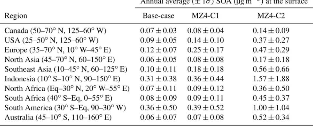
Parent VOC MOZART-4 (SAPRC 99) Oxidant α1 Kp1 α2 Kp2
Base-Case VOCs
C10Ha16(TERP) O3/OH 0.354 0.0043 0.067 0.184
C10Ha16(TERP) NO3 1.000 0.016 0.000 0.000 TOLUENEb(ARO1) OH 0.167 0.002 0.038 0.069 BIGALKc(ALK3+ALK4+ALK5) OH 0.138 0.003 0.071 0.087
MZ4-C1 VOCs
C10Ha16(TERP) O3/OH 0.289 0.008 0.086 0.205
C10Ha16(TERP) NO3 1.000 0.016 0.000 0.000
TOLUENEb(ARO1) OH 0.325 0.008 0.124 0.146 BIGALKc(ALK3+ALK4+ALK5) OH 0.100 0.150 0.047 0.080
VOCs Added in MZ4-C2
ISOP (ISOPRENE) OH 0.178 0.011 0.022 2.106 C5H8(OLE1) OH 0.078 0.005 0.006 0.167
BIGENEd(OLE2) OH 0.144 0.006 0.022 0.185
alumped monoterpenes asα-pinene;blumped aromatics as toluene;clumped alkanes with C>3 as C
5H12;
dlumped alkenes with C>3 as C
4H8.
parameters were able to represent SOA formation with the same degree of uncertainty as the VBS parameters (i.e., no additional error is introduced by the 2p-VBS fit). It there-fore can be assumed that the SOA yield and mass predictions using the Tsimpidi et al. (2010) VBS parameters and the 2p-VBS parameters produce equivalent results (in the absence of any “aging”), including temperature dependent SOA yields. The 2p-VBS fits result in a reduction from 4 “bins” (8 pa-rameters, typical for VBS) to 2 bins (4 parameters), which can be utilized in existing 2p model frameworks, such as MOZART. The MOZART SOA module does not allow for aging or processing of SOA, thus the gas-phase oxidation (beyond the initial oxidation of the parent VOC) that is of-ten represented in applications of the VBS is not considered in this work. For the precursors included in the MOZART simulations, it was determined that the 2p-VBS parameters represented available chamber data well, with the exception of isoprene. Therefore, the parameters of Henze and Sein-feld (2006) were used. In addition, the MOZART SOA mod-ule includes oxidation of monoterpenes by NO3 for which Tsimpidi et al. (2010) VBS parameters, and thus 2p-VBS pa-rameters, are not available. The monoterpene+NO3 param-eters were based on Chung and Seinfeld (2002). The devel-opment, testing, and application of 2p-VBS parameters are presented in Barsanti et al. (2013).
2.3 Model simulations
In the current study, the MOZART-4 source code was down-loaded from the University Cooperation for Atmospheric Re-search (UCAR) website (http://cdp.ucar.edu). All model sim-ulations were carried out for the entire year of 2006, and the monthly averages were analyzed. Anthropogenic emissions used for the simulation in the current study came from the POET (Precursors of Ozone and their Effects in the Tro-posphere) dataset for 2000 (Olivier et al., 2003; Granier et al., 2005). Monthly average biomass burning emissions were from the Global Fire Emissions Database, version 2 (GFED-v2) (van der Werf et al., 2006). Biogenic emis-sions of monoterpenes and isoprene are calculated online in MOZART-4 using the Model of Emissions of Gases and Aerosols from Nature (MEGAN) (Guenther et al., 2006). As described in Emmons et al. (2010) the surface and upper boundary concentrations of long-lived species (e.g., CH4and N2O) were obtained from ground- and satellite-based mea-surements.
MOZART-4 was driven by meteorology from the NCAR reanalysis of the National Centers for Environmental Pre-diction (NCEP) forecasts (Kalnay et al., 1996; Kistler et al., 2001), at a horizontal resolution of ∼2.8◦×2.8◦, with 28 vertical levels from the surface to∼2.7 hPa. This gives a
standard resolution of 128×64 grid boxes with 28 vertical
MAR
DEC
JUN
SEP
µg m
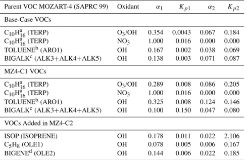
-3Fig. 1.Global distributions of monthly average SOA concentrations (µ g m−3)at the surface predicted in the base-case MOZART-4 runs for March, June, September and December of 2006.
3 Results and discussion
In this section, analyses from the base-case and updated MOZART-4 simulations are presented, followed by com-parisons with observations and previous modeling studies. Note that the first month of each simulation was excluded from the analysis to account for model spin-up time. There is no direct measurement of SOA as a component of total OA, thus observational data for global SOA levels are essen-tially non-existent. Previous studies (see for example, Lack et al., 2004; Heald et al., 2006; Liao et al., 2007; Farina et al., 2010; Jiang et al., 2012; and Lin et al., 2012) have com-pared modeled SOA to SOA determined indirectly from to-tal OA measurements. Some of these studies have also com-pared modeled SOA with reported SOA levels from relevant modeling studies. It is important to recognize that both of these techniques, comparing modeled levels with indirect de-terminations and/or with other modeling studies, have limi-tations. For example, most of the measurements are taken at specific locations over a short period of time that often do not capture the range of conditions including the influence of local emissions represented in a simulated grid, which is typically in the order of degrees (latitude×longitude) in a global chemical transport model. This makes the comparison of a global chemical transport model output with observa-tions quite challenging.
Quantification and characterization of sources of organic aerosol have always been challenging, particularly, due to utilization of different thermal–optical organic carbon quan-tification and artifact removal techniques, and handing of sampling and analytical errors including determination of sample cut sizes and detection limits. SOA concentrations are often determined indirectly using the EC tracer technique,
which also could contribute to compounding errors in com-parisons between modeled vs. calculated SOA because of the range of the EC:OC ratio that can be utilized in the
calcu-lation. Regarding model to model comparisons, model pre-dictions are also subject to errors that primarily evolve from uncertainties in emissions, meteorology, and physical and chemical parameterization techniques unique to each chemi-cal transport model. Nevertheless, such comparisons are nec-essary for model development and validation.
3.1 Modeled SOA concentrations
3.1.1 Surface concentrations
Figure 1 shows global temporal and spatial distributions of monthly average SOA concentrations (µg m−3) at the surface produced by the base-case simulations. SOA of >1.0 µg m−3is predicted in heavily forested regions includ-ing the Amazonian region in South America, equatorial re-gions in Africa, and rainforest rere-gions in Southeast Asia. The highest amount of SOA,∼3.0 µg m−3, was predicted in the
Amazonian region during the month of September, followed by∼2.0 µg m−3in Indonesia during the month of
Septem-ber and ∼2.0 µg m−3 in the equatorial region in Africa in December. The Amazonian region generally experienced
∼0.6–2.0 µg m−3of SOA in other months including March, June and December. (The highest monthly concentration,
∼9.0 µg m−3in August, was predicted in the Amazonian
re-gion and is not shown in Fig. 1.) Similarly, the rainforest regions in Southeast Asia experienced∼0.4–1.0 µg m−3 of
SOA during the months of March, June and December. The base-case model predicted∼0.2–0.8 µg m−3of SOA in the
MAR
DEC
JUN
SEP
mg m-2 day-1
mg m-2 day-1
MAR
JUN
SEP
DEC
(a)
(b)
Fig. 2.Global distributions of monthly average emission rates (mg m−2day−1)for(a)summed monoterpenes (C10H16), and(b)isoprene
(C5H8)at the surface. Examples are shown for representative months in different seasons of the year.
in the eastern and western parts of the USA only during the months of June and September. Western Europe consistently experienced∼0.2 µg m−3of SOA formation throughout the
year. In southern and eastern China, predicted SOA concen-trations varied between∼0.2 and∼1.4 µg m−3 throughout
all seasons. SOA of∼0.2 µg m−3was predicted over the
In-dian subcontinent only in December. It is important to note that the global distribution of SOA is primarily dominated by the SOA precursors emitted from biogenic sources, which can be seen from the distributions of precursor VOC emis-sions as discussed in the following paragraphs.
Figure 2a and b show global distributions of monthly av-erage surface emissions rates (mg m−2day−1) of summed monoterpenes (C10H16)and isoprene (C5H8), respectively. The plots reveal that emissions are higher in the Amazonian region in South America, mid-Africa near the Equator, north-eastern and southnorth-eastern USA, western Europe, Southeast Asia, southern and eastern China, and Australia compared
to other parts of the world. Monoterpene emissions in South America vary between∼6 and 14 mg m−2day−1throughout
the year, with highest emissions occurring during the South-ern Hemisphere spring (September) and summer (December) months. Consequently, the base-case model also predicted higher amounts of SOA in these regions (Fig. 1) during these months. Emissions in mid-Africa, Southeast Asia, and Australia vary between∼2 and 8 mg m−2day−1throughout
the year. Regions in North America and Europe emit rel-atively lower amounts of monoterpenes, <1 mg m−2day−1 for spring (March) and winter (December) months, and∼1– 6 mg m−2day−1 for summer (June) and fall (September) months.
Isoprene emissions follow similar spatial and temporal distributions to monoterpenes. Emissions in South American regions vary from∼8 to 56 mg m−2day−1, with the highest
MAR
JUN
SEP
DEC
Fig. 3.Fractional change in simulated surface SOA concentrations due to 2p parameter updates (MZ4-C1) relative to the base case.
their summer and fall months when the emissions are∼10–
40 mg m−2day−1. Consistent emissions of isoprene are also found in Southeast Asian regions throughout the year, at rates of∼8–28 mg m−2day−1. Generally, isoprene emissions are
4 to 5 times higher than the emissions of monoterpenes; thus even with a relatively low SOA yield (e.g., Lee et al., 2006), the treatment of isoprene as an SOA precursor (as in MZ4-C2) has the potential to substantially change SOA simula-tions, likely improving global and regional SOA predictions (the latter when MOZART-4 is used to generate boundary conditions).
The amount of SOA produced in the atmosphere largely depends on the concentration of precursors, availability of oxidants, and SOA yields for each of the precursor species; additionally, SOA yields depend on the amount of existing organic aerosol into which compounds can condense. Tem-perature can also play an important role in partitioning of semi-volatile organics between the gas and particle phase; cold temperatures aloft particularly favor gas-phase product condensation into particles. Global surface emissions of pri-mary organic aerosol (POA) and SOA precursors utilized in the current work are given in Table 2. A POA emission rate of 63 Tg yr−1was used for all MOZART-4 simulations, in-cluding the base case. The total SOA precursor emissions were significantly higher in the MZ4-C2 simulation than in the MZ4-C1 and base-case simulations, due to the considera-tion of isoprene, BIGENE and C3H6. The sum of VOC emis-sions acting as SOA precursors was 676 Tg yr−1 in MZ4-C2, and 199 Tg yr−1 in MZ4-C1 and the base case. Bio-genic sources constituted∼82 and∼45 %, respectively, of
the total SOA precursor emissions; of the 82 % in MZ4-C2, isoprene (ISOP) accounted for ∼84 % (with summed
monoterpenes accounting for the remaining 16 %). Lumped alkanes (BIGALK), with an emission rate of 77 Tg yr−1,
were the dominant parent VOC from anthropogenic sources followed by lumped aromatics (TOLUENE: 33 Tg yr−1), lumped alkenes (BIGENE: 9 Tg yr−1)and propene (C3H6: 6 Tg yr−1).
The change in SOA (1SOA) predicted by MZ4-C1 and MZ4-C2 was calculated as a fractional change from the base case. Figure 3 shows the distribution of the fractional change in SOA relative to the base case as predicted by MZ4-C1. Utilization of the 2p-VBS parameters resulted in significant increases in SOA over the USA in North Amer-ica, western and central Europe, and eastern China in Asia. Monthly average SOA in these regions increased by ∼1–
2 times (∼100–200 %) throughout the year with slightly
higher increases (∼200–250 %) in the month of December.
Generally, the base-case SOA concentrations in these re-gions was<1 µg m−3. A consistent SOA increase of∼50 %
in the months of September and December was seen in the South American and mid-African regions, where the base-case SOA was in the range of∼2–3 µg m−3for those
months. Increased SOA in continental North America, Eu-rope, and Asia indicates that anthropogenic precursors such as toluene (TOLUENE) and lumped alkanes (BIGALK) can lead to significant SOA formation, even as represented in a global model, depending on the parameters used. SOA pro-duction nearly mimics the pattern of emissions, i.e., SOA is predominantly formed where the emission sources are. Monoterpenes in the southeast coastal regions of Australia are emitted at a rate of∼1.0 mg m−2day−1in the summer
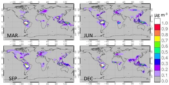
Table 2.Global surface emissions of POA and SOA precursors from anthropogenic and biogenic sources.
Type/Species Emissions (Tg yr−1)
POA (hydrophobic+hydrophilic)∗ 63
Anthropogenic
TOLUENE(C7H8: lumped aromatics) 33
BIGALK(C5H12: lumped alkanes with C>3) 77
BIGENE (C4H8: lumped alkenes with C>3) 9
C3H6(propene) 6
Biogenic
C10H16(lumped monoterpenes asα-pinene) 89
ISOP (C5H8: isoprene) 462
∗A multiplication factor of 1.4 (Griffin et al., 1999) was used to convert primary organic carbon (POC) to primary
organic aerosol (POA) mass.
Northern Hemisphere (Fig. 3) where the base-case SOA con-centrations are generally negligible. Replacing the default SOA parameters with the 2p-VBS parameters increased pre-dicted SOA mass concentrations by 0.1–0.2 µg m−3 in the eastern USA, 0.2–0.6 µg m−3in Europe, 0.3–0.9 µg m−3 in eastern China, and 0.2–0.4 µg m−3in the Amazon and South-east Asia throughout the year. Figure 4 shows the fractional change in monthly average SOA relative to the base case as predicted by MZ4-C2. SOA increased over some areas in the eastern USA, western Europe, South and Southeast Asia, and China by as much as∼2–4 times (∼200–400 %); in
MZ4-C2, predicted SOA concentrations were ∼0.1–0.2 µg m−3
throughout the year, except for the month of September, which showed higher increases (up to ∼600 %) in some
parts of the USA, China, and South and Southeast Asia. The highest increase of SOA (∼16–28 times the base case)
was predicted in northwestern Australia during the months of September and December. In these regions, greater increases in SOA were predicted due to the contribution of isoprene in September and December (which follows the pattern of isoprene emissions at these times of the year in these re-gions). Given the absence of isoprene as an SOA precursor in the base case, the corresponding base-case concentrations of SOA in these regions were usually low∼0.01–0.04 µg m−3. MZ4-C2 predicted∼400–600 % increases in some hotspots
in the Amazonian regions in South America throughout the year. Similar increases were also seen in middle and south-ern parts of Africa during the months of March, September and December. Again, these patterns of increased SOA fol-lowed the patterns of isoprene emissions during correspond-ing months. The difference in plots between the MZ4-C2 and base-case simulations (not shown) indicated significant in-creases in SOA concentrations (>1.0 µg m−3)in the equato-rial Africa, Amazonian region, eastern China, and Southeast Asia, due to high emissions of biogenic precursors, namely isoprene, in these regions.
Table 3 contains regionally averaged annual SOA con-centrations at the surface with ±1σ, which represents both spatial and temporal variations, for several geographic areas around the world for all three model simulations. The area coordinates were adopted from Emmons et al. (2010). The regional averages were calculated based on SOA concentra-tions in all grid cells over land within the specified coordi-nates using the global land-mask field. The base-case annual average SOA concentrations were generally high in regions with higher emissions from biogenic sources, in this case, monoterpenes only (e.g., Fig. 1). With MZ4-C1 (SOA pa-rameter updates) the concentration of SOA increased from the base case between ∼8 and 108 %. It is interesting to
note that the changes were usually greater for areas where SOA was low, but heavily dominated by anthropogenic emis-sions. For example, USA, Europe, North Asia and Southeast Asia showed relatively higher SOA mass increases, ∼16–
108 % (over the base case). In comparison, SOA mass in-creases in regions in South America, Indonesia, Africa, and Australia were generally lower, ∼8–16 %. (These changes due to parameter updates also are reflected in Fig. 3.) For the MZ4-C2 simulations (SOA parameter updates and addi-tional SOA precursors) regionally averaged annual SOA in-creased from the base case by as much as∼90–600 % (or
∼0.9–6 times). The increase was attributed mostly to the
consideration of isoprene as an SOA precursor, which ac-counted for∼99 % of the increased global SOA production
in MZ4-C2, compared to the two anthropogenic precursors, namely propene (C3H6)and lumped big alkenes (BIGENE), which accounted for the remaining∼1 %. The standard
MAR
JUN
SEP
DEC
Fig. 4.Fractional change in simulated surface SOA concentrations due to 2p parameter updates and consideration of additional SOA precur-sors (MZ4-C2) relative to the base case.
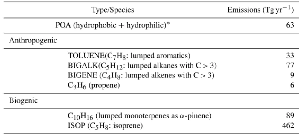
Table 3.Regionally averaged annual SOA concentrations at the surface for the year 2006.
Annual average (±1σ )SOA (µg m−3)at the surface
Region Base-case MZ4-C1 MZ4-C2
Canada (50–70◦N, 125–60◦W) 0.07±0.03 0.08±0.04 0.14±0.09 USA (25–50◦N, 125–60◦W) 0.09±0.05 0.14±0.10 0.37±0.27 Europe (35–70◦N, 10◦W–45◦E) 0.12±0.07 0.25±0.17 0.47±0.29 North Asia (45–70◦N, 60–150◦E) 0.06±0.05 0.08±0.08 0.17±0.18 Southeast Asia (10–45◦N, 60–125◦E) 0.10±0.11 0.18±0.18 0.56±0.66 Indonesia (10◦S–10◦N, 90–150◦E) 0.31±0.38 0.36±0.44 1.57±1.88 North Africa (Eq–30◦N, 20◦W–55◦E) 0.07±0.11 0.09±0.12 0.36±0.50 South Africa (40◦S–Eq, 0–55◦E) 0.08±0.09 0.09±0.11 0.45±0.37 South America (30◦S–Eq, 90–30◦W) 0.36±0.50 0.39±0.52 1.00±1.04 Australia (45–10◦S, 110–160◦E) 0.06±0.07 0.07±0.08 0.52±0.34
3.1.2 Vertical profiles
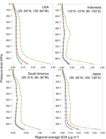
Several past and recent studies found that global chemical transport models poorly represent observed concentrations of SOA in the vertical direction (see for example, Heald et al., 2005, 2011; and Lin et al., 2012). Efforts were made in the current study to examine how changes in SOA at the surface, driven by updates to the SOA module, translated to the other vertical layers. MOZART-4 has 28 vertical layers extending up to∼2.7 hPa (∼30 km) above ground. Figure 5 shows ver-tical profiles of regionally averaged annual SOA concentra-tions for four regions: USA, Indonesia, South America and Japan. The figure shows that updating the SOA parameters (MZ4-C1) had little effect on the vertical profiles compared to the base case; whereas, treating the additional SOA precur-sors (MZ4-C2), namely isoprene, had a significant effect on vertical profiles. The reason for the increase in SOA aloft is
likely two-fold. First, as noted by Henze and Seinfeld (2006), is the magnitude of isoprene emissions; and second, is the relatively high yield/low volatility of isoprene SOA prod-uct 1, as determined by the fittedαandKpvalues shown in Table 1. MZ4-C2-predicted SOA increased by∼160,∼300, ∼170 and∼150 % in the free troposphere (between 801.40– 435.70 hPa,∼2–6 km) for USA, Indonesia, Japan, and South America from the base-case annual average of 0.03, 0.08, 0.03, and 0.12 µg m−3, respectively.
3.1.3 Global budgets
Table 4.Global SOA budget estimates.
Model versions Removal (Tg yr
−1)
Production (Tg yr−1) Lifetime (days) Burden (Tg) Dry Wet
Base case 1.1 4.7 5.8 13.6 0.22
Updated–MZ4-C1 1.4 5.2 6.6 13.1 0.24 Updated–MZ4-C2 4.7 14.4 19.1 11.2 0.59
Regional average SOA (g m-3)
P
ressu
re
lev
e
l
(h
P
a
)
USA (2550N, 12560W)
Indonesia (10S10N, 90150E)
South America (300S, 9030W)
Japan (3040N, 120140E)
Fig. 5.Vertical distributions of regionally averaged annual SOA concentrations (µg m−3). Simulated SOA concentrations for the base case are represented by open diamonds (blue); open squares (red) represent updated version, MZ4-C1 (updated 2p parameters), and open circles (green) represent updated version, MZ4-C2 (up-dated 2p parameters and additional parent VOCs).
estimated in MZ4-C1 and MZ4-C2, respectively. Updates to the SOA parameters and inclusion of additional precur-sors clearly enhanced SOA production, which also increased atmospheric burdens by 8 and 168 %, respectively, from the base case. Among the three newly treated parent VOC species, isoprene contributed∼99 % to additional
produc-tion of atmospheric SOA (through OH oxidaproduc-tion) and for
∼65 % of total atmospheric SOA production. Comparable
modeling studies reported that isoprene alone can generate up to 15–75 % of atmospheric SOA (see for example, Heald
et al., 2006; Henze and Seinfeld, 2006; Hoyle et al., 2007; Liao et al., 2007; and Tsigaridis and Kanakidou, 2007). The SOA lifetime estimated from the base-case simulation was 13.6 days; estimated SOA lifetime for MZ4-C1 and MZ4-C2 was 13.1 and 11.2 days, respectively. The shorter calculated lifetime for MZ4-C2 (−18 % relative to the base case) was
likely due to the inclusion of isoprene as an SOA precur-sor. The atmospheric lifetimes of biogenic precursors (∼h)
are generally shorter than anthropogenic precursors (∼days) (Farina et al., 2010); thus, anthropogenic precursors are more likely to be transported to higher altitudes prior to the forma-tion of SOA, where dry and wet deposiforma-tion are less efficient (Lin et al., 2012). In MZ4-C2, much of the enhanced SOA formation (due to isoprene) was within the first few layers (within ∼500 m above ground, see Fig. 4) where dry and
wet depositions are very effective. Two additional simula-tions were carried out to illustrate this lifetime effect. With anthropogenic precursors only in the SOA module, the dicted SOA lifetime was 17.6 days, compared to the pre-dicted SOA lifetime of 11.2 days for the biogenic only case. The biogenic only simulation was essentially equivalent to MZ4-C2, with isoprene being the largest contributor to SOA production. The predicted SOA mass concentrations between the anthropogenic only simulation (lifetime ∼17.6 days), the base case (lifetime∼13.6 days) and MZ4-C1 (lifetime
∼13.1 days) were similar in magnitude (as compared with MZ4-C2); however, the presence of the biogenic (specifically monoterpenes) precursors in the base-case and MZ4-C1 sim-ulations resulted in greater SOA formation at the surface, and thus an increase in deposition and decrease in SOA lifetime.
3.2 Model evaluation
0 2 4 6 8 10
0 2 4 6 8 10 12
Modele
d
O
A
(µg m
-3)
Measured OA (µg m-3)
Asia
Europe
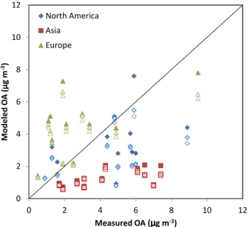
Fig. 6.Modeled vs. measured OA mass concentrations at several locations in North America, Europe and Asia. The solid fill sents MZ4-C2, patterned fill represents MZ4-C1, and no fill repre-sents MZ4 base-case simulations. Measured data were adapted from Zhang et al. (2007).
from 1.3; Liousse et al., 1996 to 2.2; and Zhang et al., 2005) the choice of the OM:OC value is one source of uncertainty in model evaluation. The value of 1.4 used here is on the lower end of the global mean values and thus may bias results toward under-prediction if POA is converted from primary organic carbon (POC) and/or over-prediction if SOA is con-verted to secondary organic carbon (SOC) in the analysis. In the current version of MOZART4, SOA yields are calculated only for high NOXpathways, which may bias SOA concen-trations, particularly in regions under low NOX conditions. This could be another source of uncertainty when comparing modeled concentrations with observations. However, the dis-cussion of modeled concentrations in Sect. 3.1 indicated that because of the overwhelming contribution of isoprene (for which high and low NOXparameters currently do not exist) to SOA on the global scale, the bias from high NOX parame-ters are less likely to be significant in the current analysis.
3.2.1 Surface SOA
Surface measurement data of OA at several locations in North America, Europe and Asia were obtained from Zhang et al. (2007). The list of the dataset names, categories and geographic locations of sampling sites, and the duration of each measurement campaign can be found in Zhang et al. (2007). Corresponding model results from the MZ4-C2, MZ4-C1, and the base-case simulations were then compared with observations. Figure 6 shows a scatter plot of modeled vs. measured OA concentrations. The solid, patterned, and
The figure shows that even with the updated 2p parame-ters and added precursors, MOZART-4 (MZ4-C2) under-estimated (NMB (normalized mean bias):−70 %) measured
OA concentrations at all remote and urban sites in Asia (solid squares), and the model has showed slight improvement over the base-case simulation (NMB:−76 %). The severe
under-estimation at sites in Asia is perhaps due to the fact that most of the measurements were taken at rural sites that were likely impacted by pollutants transported from nearby re-gions over a short period of time, but the model perhaps did not capture those episodic pollution events in the simu-lation. The updated model over-estimated measurements at most urban sites in Europe (solid and patterned triangles, NMB: 63 and 49 %), even the base-case simulation (open tri-angles, NMB: 43 %) showed over-estimation in those sites. The over-estimation of total OA could be attributed to the fact that the model grids where the measurements took place perhaps did not have representative conditions for emissions and meteorology. The OM:OC ratio of 1.4 applied in the
analysis might not be appropriate for Europe. Measured OA concentrations at several sites in North America (solid dia-monds), however, were relatively better reproduced by the MZ4-C2 (NMB:−27 %) simulation compared to the
MZ4-C1 (NMB: −41 %) and base-case (NMB: −44 %)
simula-tions in the current study. Therefore, only the MZ4-C2 results will be further compared with observations and previously published modeling results.
MZ4-C2 predicted increased SOA mass concentrations at the surface in North America (particularly in the eastern USA) and Europe during the summer months of June, July and August, when biogenic emissions are at their peak. Us-ing GEOS-Chem, Liao et al. (2007) predicted climatologi-cal average (2001–2003) summertime SOA concentrations of∼0.5–2 and∼0.5–1 µg m−3from isoprene and
monoter-pene precursors over the southeastern and northeastern USA, respectively. In this study, predicted summertime SOA con-centrations were ∼0.9–1.3 and ∼1.3–1.4 µg m−3 over the
northeastern and southeastern USA, respectively. Farina et al. (2010) reported that the GISS II GCM predicted SOA reasonably well over Europe. Estimated monthly average OM concentrations were between 8.5 and 8.9 µg m−3while the observed monthly average was 6.9 µg m−3for the period 2002–2003. In the present study, the modeled monthly aver-age OM for the same region (Europe) was∼5.0 µg m−3for the year 2006.
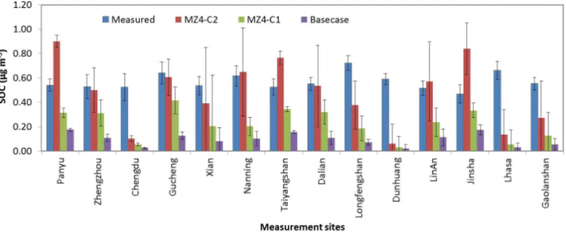
Fig. 7.Measured vs. modeled comparison of SOC at various measurement sites in China. Measured data were obtained from Zhang et al. (2012).
sites, categories and their geographic locations can be found in Zhang et al. (2012). The error bars in the plot represent
±1σ of annual average SOC concentrations. The compari-son emphasizes that the MZ4-C2 produced SOA mass con-centrations relatively well at 8 out of 14 sites compared to MZ4-C1 and base case, where ±1σ between measured and modeled averages overlap. Robinson et al. (2011) reported a measured OM concentration of 0.74 µg m−3 at the sur-face in the Malaysian Borneo (4.981◦N, 117.844◦E) during the oxidant and particulate photochemical processes above a Southeast Asian rainforest (OP3)/Aerosol Coupling in the Earth’s System (ACES) project (June–July 2008). For these two months in summer, MZ4-C2 predicted a monthly aver-age OM of∼2.3 µg m−3of which∼58 % was attributable to SOA derived from isoprene oxidation. This apparent over-prediction may be explained by an erroneously high isoprene SOA yield or unrepresentative 2p parameters (for the mod-eled ambient conditions), the assumed value of the OM:OC
ratio and/or the over-estimation of modeled emission rates utilized in the current study. In a recent modeling study, Jiang et al. (2012) estimated annual average SOA concen-trations of∼2.78 and∼2.92 µg m−3for areas within
south-ern China (22–26◦N, 100–115◦E) and central China (25– 35◦N, 103–120◦E), respectively, for the year 2006 using a regional-scale model, WRF-Chem (Weather Research and Forecasting–Chemistry). MZ4-C2 predicted annual average SOA concentrations of 1.11±0.59 and 0.88±0.42 µg m−3 for southern and central China, respectively. The SOC:OC ratio predicted by MZ4-C2 was∼17 % compared to∼16 % reported by Jiang et al. (2012) in northern China, while ob-served SOC:OC ratios of ∼26–59 % have been reported
for the Beijing area (Dan et al., 2004; Chan et al., 2005; Duan et al., 2005; Lin et al., 2009). Thus, the updated ver-sion of MOZART, MZ4-C2, generally predicted SOA con-centrations comparable to other similar modeling studies for regions in China, but over-predicted measured summertime
monthly average concentrations in the forested region in Southeast Asia.
Recall that MZ4-C2 predicted generally high SOA con-centrations in and around the Amazonian regions in South America. Like regions in Asia, OA measurement data in the Amazonian region are also limited and sporadic. Gilardoni et al. (2011) reported a measured OM concentration of 1.70 µg m−3at the surface in the Amazonian basin during the wet season (February–June); Chen et al. (2009) reported con-centrations of submicron (<1 µm) OM during the February– March period of 0.7 µg m−3. An average OM concentra-tion of ∼2.15 µg m−3 was predicted in the current study for the Amazonian region during the wet season. Another modeling study by Lin et al. (2012) predicted an average OM of ∼3.5 µg m−3for the same region and season. The
modeled concentrations from the current study and Lin et al. (2012) appear to be over-estimating OM in this region. Such over-estimations could be due to an over-estimation of the isoprene SOA yield (for the ambient conditions modeled) and/or an over-estimation of the emissions (of SOA precur-sors and/or POA) in the region. This discrepancy may also be attributed to different meteorology being used in simulations as compared with the meteorology during the measurement periods.
3.2.2 Vertical profiles
prehensive analysis of OA vertical profiles from 17 field cam-paigns from 2001–2009 (including the two mentioned above) in order to validate model performance on a global scale. In this study, comparisons of modeled vertical profiles were limited to the early field campaigns over the northwest Pa-cific (ACE-Asia) and the northeast of North America (ITCT-2K4).
Heald et al. (2005) reported that GEOS-Chem under-predicted OC, of which SOA is a dominant component, by as much as 10–100 times during the ACE-Asia (2001) study near the coast of Japan (23–43◦N, 120–145◦E). MZ4-C2 in the current study predicted a seasonal (April–May) OC aerosol mass of 0.58±0.24 µg C m−3in the free troposphere (FT) averaged over all the grid cells within the area bound-ary at model resolution, of which∼16 % was attributed to SOA; the observed seasonal average OC mass along the fight paths was 3.3±2.8 µg C m−3. The predicted OC mass
concentration in the current study showed a significant im-provement from the reported maximum modeled value of 0.30±0.3 µg C m−3by Heald et al. (2005) averaged over the
grid cells along the flight paths. It is worth noting that Heald et al. (2005) treated monoterpenes as the only biogenic VOC precursor, whereas MZ4-C2 includes both monoterpenes and isoprene. The model prediction in the current study is com-parable with the FT average modeled OC aerosol mass of
∼0.7 µg C m−3(STP, standard temperature and pressure)
re-ported by Lin et al. (2012) for the ACE-Asia field campaign; similarly to this work, Lin et al. (2012) considered isoprene and monoterpenes as major biogenic precursors.
During the ITCT-2K4 campaign (25–55◦N, 270–310◦E) over summer months July-August, aircraft measurements in-cluded those within a large plume that originated from bo-real forest fires in Alaska and Canada. Chemical transport models often miss such plumes resulting in significant under-prediction of OM. Heald et al. (2006) reported observed water soluble organic carbon (WSOC) concentrations of 0.9±0.9 µg C m−3in the FT averaged along the flight paths
outside of the boreal forest fire plume, and a corresponding modeled WSOC concentration of 0.7±0.6 µg C m−3
aver-aged from only grid cells along the flight paths at model resolution. In the current study, MZ4-C2 predicted seasonal WSOC aerosol mass of 0.36±0.15 µg C m−3, of which 21 % was attributable to SOA, in the FT averaged from all grid cells within the region boundary specified. Both the current study and Heald et al. (2006) included monoterpenes and isoprene as major biogenic precursors with similar emission strengths; the apparent difference in model prediction may have been due to differences in how the average results are calculated.
There is significant uncertainty in global SOA budget esti-mates. A wide range of SOA production rates, measurement and model based, can be found in the literature. For example, Goldstein and Galbally (2007) estimated SOA production of 510–910 Tg C yr−1based on a top-down VOC mass balance approach. Global model estimates of SOA production based on bottom-up approaches typically span a lower range, from 6.74 Tg yr−1 (Goto et al., 2008) to 96 Tg yr−1 (Guillaume et al., 2007). The differences in SOA production and atmo-spheric burden among these model estimates predominantly come from differences in source emissions, choice of SOA parameters, and treatment of parent VOCs in SOA mod-els. Nevertheless, inter-comparisons between models provide useful information for testing and validating model perfor-mance. Thus SOA production, lifetime and corresponding atmospheric burden estimates from the current study were compared with estimates from other global chemical trans-port models.
MAR
JUN
SEP
DEC
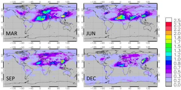
Fig. 8.Global distributions of monthly average total AOD for the base-case MOZART-4 simulations.
the observationally constrained top-down estimates (50– 380 Tg yr−1)of Spracklen et al. (2011).
3.3 Aerosol optical depth
In MOZART-4, the AOD is calculated only when the photol-ysis rates are calculated (zenith angle, SZA is less than 90◦), so the monthly average total AOD was scaled by the fraction of daylight hours per day estimated in the model. Total AOD reflects contributions from aerosols originating from primary and secondary organics, sea salt, sulfate, nitrate, and dust. The FTUV module in MOZART-4 generates 17 wavelength bins for each of which optical properties of those aerosol types are utilized. The optical and physical property data for each of those types of aerosol were obtained mostly from OPAC dataset by Hess et al., 1998. Except dust, other aerosol types including sulfate, nitrate, organic carbon, black carbon, SOA and sea salt are treated for water uptake in the AOD cal-culation in the model. In the absence of adequate data, SOA is treated similarly to OC in AOD calculations.
Figure 8 shows the modeled spatial distribution of to-tal AOD for the base-case MOZART-4 simulations. The monthly averaged total AOD presented here includes con-tributions from primary and secondary OC, BC, dust, sea salt, and sulfate and nitrate particles. As shown in Fig. 8, AOD is generally higher for the Northern Hemisphere than the Southern Hemisphere, supporting that primary anthro-pogenic particulate emissions (e.g., BC) and dust are the largest contributors to modeled AOD; this is in contrast to the significant contribution of biogenic emissions to total partic-ulate loadings through SOA formation. High AOD (>∼2.0)
over Northern Africa reflects large contributions (∼80 %)
from dust particles, and over southeastern China from anthro-pogenic sources (>∼90 %) including BC, sulfate, nitrate
and OC. However, the contribution of OC to total AOD is generally<∼20 % in the modeled regions (Table 5).
The fractional increase of total AOD in the updated model simulation (MZ4-C2) from the base case was calculated. The increase in AOD was in the range of∼1–7 % in areas where
SOA production also increased due to treatment of addi-tional SOA precursor VOCs. To illustrate further that anthro-pogenic aerosols dominate AOD, regionally averaged annual AOD was calculated for several regions including over ma-jor oceans of the world. Table 5 contains regionally aver-aged base-case annual total AOD, contributions from POA and SOA, and change in total AOD attributed to additional SOA formed in the MZ4-C2 simulations. The table contains total AOD analysis for the regions for which SOA was also averaged annually (Table 3). Additionally, annual total AOD results over oceans are presented. Note that the AOD over oceans was calculated using ocean only grid cells within the boundary coordinates. Generally, AOD was much higher over land compared to over oceans because sources are lo-cated over land. The base-case model predicted the high-est annual average total AOD of 0.73 over North Africa, of which ∼80 % is attributed to dust; only 3 % is attributed to POA and SOA. MZ4-C2 predicted POA and SOA con-tributed∼3–21 % to total AOD over the regions considered in the current study. Regionally averaged annual total AOD increased by∼0.6–8.2 % due to additional SOA formed in
the MZ4-C2 simulation. The model predicted that AOD in-creased over areas where SOA also inin-creased from the base-case prediction. For example, Australia, Indonesia and South America experienced∼750,∼400 and ∼300 % increases
in SOA, which contributed to increases in total AOD by
∼7.7, 4.4, and 6.2 %, respectively. Increased SOA resulted
in a corresponding∼2.3–8.2 % increase in AOD over the
Base case MZ4-C2
Region Total POA and SOA Increase in total AOD contributions to AOD attributed total AOD (%) to SOA (%)
Canada (50–70◦N, 125–60◦W) 0.23 7 0.9 (0.1–2.1) USA (25–50◦N, 125–60◦W) 0.32 6 1.2 (0.3–3) Europe (35–70◦N, 10◦W–45◦E) 0.60 5 0.6 (0.1–1.8) North Asia (45–70◦N, 60–150◦E) 0.38 7 0.6 (0.1–1.4) Southeast Asia (10–45◦N, 60–125◦E) 0.62 5 1.8 (1.0–2.4) Indonesia (10◦S–10◦N, 90–150◦E) 0.18 21 4.4 (1.1–15.7) North Africa (Eq–30◦N, 20◦W–55◦E) 0.73 3 2.9 (1.3–5.3) South Africa (40◦S–Eq, 0–55◦E) 0.14 19 2.8 (1.3–8.2) South America (30◦S–Eq, 90–30◦W) 0.15 14 6.2 (2.6–13.3) Australia (45–10◦S, 110–160◦E) 0.14 9 7.7 (3.6–30.4) North Pacific Ocean (Eq–60◦N, 135◦E–100◦W) 0.20 6 2.3 (1.2–3.2) North Atlantic Ocean (Eq–60◦N, 0–80◦W) 0.39 3 2.9 (1.5–3.4) South Pacific Ocean (45◦S–Eq, 150◦E–80◦W) 0.08 6 8.2 (4.5–17.6) South Atlantic Ocean (45◦S–Eq, 60◦W–15◦E) 0.13 13 4.1 (2.2–8.9) Indian Ocean (45◦S–30◦N, 30–150◦E) 0.24 7 4.1 (2.2–6.9)
experienced the highest AOD increase of 8.2 % predicted by MZ4-C2.
There has been little effort to evaluate AOD predicted by MOZART-4, with the exception of the Emmons et al. (2010) study. In that study, MODIS retrievals were used to evalu-ate predicted monthly average total AOD over major oceans for several years of retrievals/model simulations. Compar-isons for 2006 showed that the modeled AOD fell within the variability bounds of retrieved total AOD for each region of interest. Predicted monthly average total AOD (the base-case MOZART-4 AOD in this work) agreed quite well with observations over the North Pacific Ocean, under-estimated AOD over the South Pacific, South Atlantic, and Indian oceans, and over-estimated AOD over the North Atlantic Ocean. In the current study, MZ4-C2 predicted∼2–8 %
in-creases in the annual total AOD over these oceans, sug-gesting that the model updates bring the under-estimated monthly average AOD closer to observations, except over the North Atlantic Ocean where the base-case model already over-estimated AOD. The comparison between MZ4-C2 and Lee and Chung’s (2013) best estimated AOD shows that the model in the current study slightly over-estimated AOD over land regions. Lee and Chung (2013) combined AOD mea-surements from AERONET, MISR, MODIS and GOCART data, and presented their best estimated AODs of 0.15–0.20, 0.13–0.30, 0.3–0.8 and 0.10–0.15, over Indonesia, South America, North Africa, and Australia, respectively. As can be seen from Table 5, the updated model estimated AODs fall within the Lee and Chung (2013) ranges for these regions.
4 Conclusions
The secondary organic aerosol (SOA) module in the MOZART-4 global chemical transport model was updated by replacing the existing two-product (2p) parameters with those obtained from recent two-product volatility basis set (2p-VBS) fits (MZ4-C1), and by adding isoprene (C5H8), propene (C3H6)and lumped alkenes with C>3 (BIGENE) as precursor VOCs (volatile organic compounds) contribut-ing to SOA formation (MZ4-C2) in the current study. Com-parisons were made between the model simulations (base case and the two modified cases, MZ4-C1 and MZ4-C2) and with other model predictions and ambient observations. The updates to the SOA model largely improved predictions of SOA mass concentrations at the surface relative to pre-dicted in the base-case MOZART4 model. Relative to the base-case simulation, MZ4-C1 predicted higher concentra-tions in regions where anthropogenic emissions were dom-inant, while MZ4-C2 predicted higher concentrations in re-gions where biogenic emissions were dominant. The compar-isons between modeled and measured OA (organic aerosol) at several rural and urban sites in the Northern Hemisphere showed that the updates to MOZART4 still resulted in under-prediction of surface OA mass concentration at both rural and urban sites (Table S3). MZ4-C2, however, clearly showed significant improvements over the base-case and MZ4-C1 predictions as indicated by fractional bias (FB) calculations at both rural (MZ4-C2, FB:−19 % vs. MZ4-C1, FB:−36 %
and base case, FB:−40 %), and urban (MZ4-C2, FB:−26 %
The modifications to the SOA module in MOZART-4 are scientifically relevant and important for future studies utiliz-ing MOZART-4, or chemical transport models with a sim-ilarly configured SOA module, including those directed at global SOA and total OA budget estimations and pollution source attribution. These modifications if adopted, will also lead to improvements in regional air quality models where MOZART output is used for boundary conditions.
Acknowledgements. This work was supported by the Cooley Family Fund for Critical Research of the Oregon Community Foundation and Research and Sponsored Projects, and the Institute of Sustainable Solutions at Portland State University.
Edited by: O. Boucher
References
Andreae, M. O. and Crutzen, P. J.: Atmospheric aerosols: Biogeo-chemical sources and role in atmospheric chemistry, Science, 276, 152–158, doi:10.1126/science.276.5315.1052, 1997. Barsanti, K. C., Carlton, A. G., and Chung, S. H.: Analyzing
ex-perimental data and model parameters: implications for predic-tions of SOA using chemical transport models, Atmos. Chem. Phys. Discuss., 13, 15907–15947, doi:10.5194/acpd-13-15907-2013, 2013.
Barth, M. C., Rasch, P. J., Kiehl, J. T., Benkovitz, C. M., and Schwartz, S. E.: Sulfur chemistry in the National Center for At-mospheric Research Community Climate Model: Description, evaluation, features, and sensitivity to aqueous chemistry, J. Geo-phys. Res., 105, 1387–1415, 2000.
Brasseur, G. P., Hauglustaine, D. A., Walters, S., Rasch, P. J., Muller, J. F., Granier, C., and Tie, X. X.: MOZART, a global chemical transport model for ozone and related chemical trac-ers 1. Model description, J. Geophys. Res., 103, 28265–28289, doi:10.1029/98jd02397, 1998.
Chan, C. Y., Xu, X. D., Li, Y. S., Wong, K. H., Ding, G. A., Chan, L. Y., and Cheng, X. H.: Characteristics of ver-tical profiles and sources of PM2.5, PM10 and carbona-ceous species in Beijing, Atmos. Environ., 39, 5113–5124, doi:10.1016/j.atmosenv.2005.05.009, 2005.
Chen, Q., Farmer, D. K., Schneider, J., Zorn, S. R., Heald, C. L., Karl, T. G., Guenther, A., Allan, J. D., Robinson, N., Coe, H., Kimmel, J. R., Pauliquevis, T., Borrmann, S., Poeschl, U., An-dreae, M. O., Artaxo, P., Jimenez, J. L., and Martin, S. T.: Mass spectral characterization of submicron biogenic organic parti-cles in the Amazon Basin, Geophys. Res. Lett., 36, L20806, doi:10.1029/2009gl039880, 2009.
Chin, M., Ginoux, P., Kinne, S., Torres, O., Holben, B. N., Dun-can, B. N., Martin, R. V., Logan, J. A., Higuarish, A., and Naka-jima, T.: Tropospheric aerosol optical thickness from the GO-CART model and comparisons with satellite and sun photometer measurements, J. Atmos. Sci., 59, 461–483, 2002.
Chung, S. H. and Seinfeld, J. H.: Global distribution and climate forcing of carbonaceous aerosols, J.Geophys. Res., 107, 4407, doi:10.1029/2001jd001397, 2002.
Claeys, M., Wang, W., Ion, A. C., Kourtchev, I., Gelencser, A., and Maenhaut, W.: Formation of secondary organic aerosols from isoprene and its gas-phase oxidation products through reac-tion with hydrogen peroxide, Atmos. Environ., 38, 4093–4098, doi:10.1016/j.atmosenv.2004.06.001, 2004.
Clarisse, L., Fromm, M., Ngadi, Y., Emmons, L., Clerbaux, C., Hurtmans, D., and Coheur, P.-F.: Intercontinental transport of anthropogenic sulfur dioxide and other pollutants: An infrared remote sensing case study, Geophys. Res. Lett., 38, L19806, doi:10.1029/2011gl048976, 2011.
Dan, M., Zhuang, G. S., Li, X. X., Tao, H. R., and Zhuang, Y. H.: The characteristics of carbonaceous species and their sources in PM2.5 in Beijing, Atmos. Environ., 38, 3443–3452,
doi:10.1016/j.atmosenv.2004.02.052, 2004.
Delfino, R. J., Sioutas, C., and Malik, S.: Potential role of ul-trafine particles in associations between airborne particle mass and cardiovascular health, Environ. Health Persp., 113, 934–946, doi:10.1289/ehp.7938, 2005.
Donahue, N. M., Robinson, A. L., Stanier, C. O., and Pandis, S. N.: Coupled partitioning, dilution, and chemical aging of semivolatile organics, Environ. Sci. Technol., 40, 2635–2643, doi:10.1021/es052297c, 2006.
Duan, F. K., He, K. B., Ma, Y. L., Jia, Y. T., Yang, F. M., Lei, Y., Tanaka, S., and Okuta, T.: Characteristics of carbona-ceous aerosols in Beijing, China, Chemosphere, 60, 355–364, doi:10.1016/j.chemosphere.2004.12.035, 2005.
Dunlea, E. J., DeCarlo, P. F., Aiken, A. C., Kimmel, J. R., Peltier, R. E., Weber, R. J., Tomlinson, J., Collins, D. R., Shinozuka, Y., McNaughton, C. S., Howell, S. G., Clarke, A. D., Emmons, L. K., Apel, E. C., Pfister, G. G., van Donkelaar, A., Martin, R. V., Millet, D. B., Heald, C. L., and Jimenez, J. L.: Evolution of Asian aerosols during transpacific transport in INTEX-B, At-mos. Chem. Phys., 9, 7257–7287, doi:10.5194/acp-9-7257-2009, 2009.
Emmons, L. K., Walters, S., Hess, P. G., Lamarque, J.-F., Pfister, G. G., Fillmore, D., Granier, C., Guenther, A., Kinnison, D., Laepple, T., Orlando, J., Tie, X., Tyndall, G., Wiedinmyer, C., Baughcum, S. L., and Kloster, S.: Description and evaluation of the Model for Ozone and Related chemical Tracers, version 4 (MOZART-4), Geosci. Model Dev., 3, 43–67, doi:10.5194/gmd-3-43-2010, 2010.
Farina, S. C., Adams, P. J., and Pandis, S. N.: Modeling global secondary organic aerosol formation and processing with the volatility basis set: Implications for anthropogenic secondary organic aerosol, J. Geophys. Res., 115, D09202, doi:10.1029/2009jd013046, 2010.
aerosol in the Amazon basin, Atmos. Chem. Phys., 11, 2747– 2764, doi:10.5194/acp-11-2747-2011, 2011.
Goldstein, A. H. and Galbally, I. E.: Known and unexplored organic constituents in the earth’s atmosphere, Environ. Sci. Technol., 41, 1514–1521, doi:10.1021/es072476p, 2007.
Goto, D., Takemura, T., and Nakajima, T.: Importance of global aerosol modeling including secondary organic aerosol formed from monoterpene, J. Geophys. Res., 113, D07205, doi:10.1029/2007jd009019, 2008.
Granier, C., Guenther, A., Lamarque, J., Mieville, A., Muller, J., Olivier, J., Orlando, J., Peters, J., Petron, G., Tyndall, G., and Wallens, S.: POET, a database of surface emissions of ozone precursors, available at: http://www.aero.jussieu.fr/projet/ ACCENT/POET.php (last access: August 2008), 2005.
Griffin, R. J., Cocker, D. R., Flagan, R. C., and Seinfeld, J. H.: Organic aerosol formation from the oxidation of biogenic hydrocarbons, J. Geophys. Res., 104, 3555–3567, doi:10.1029/1998jd100049, 1999.
Guenther, A., Karl, T., Harley, P., Wiedinmyer, C., Palmer, P. I., and Geron, C.: Estimates of global terrestrial isoprene emissions using MEGAN (Model of Emissions of Gases and Aerosols from Nature), Atmos. Chem. Phys., 6, 3181–3210, doi:10.5194/acp-6-3181-2006, 2006.
Guillaume, B., Liousse, C., Rosset, R., Cachier, H., Van Velthoven, P., Bessagnet, B., and Poisson, N.: ORISAM-TM4: a new global sectional multi-component aerosol model including SOA forma-tion – Focus on carbonaceous BC and OC aerosols, Tellus B, 59, 283–302, doi:10.1111/j.1600-0889.2006.00246.x, 2007. Hack, J. J.: Parameterization of moist convection in the
Na-tional Center for Atmospheric Research community cli-mate model (CCM2), J. Geophys. Res., 99, 5551–5568, doi:10.1029/93jd03478, 1994.
Hallquist, M., Wenger, J. C., Baltensperger, U., Rudich, Y., Simp-son, D., Claeys, M., Dommen, J., Donahue, N. M., George, C., Goldstein, A. H., Hamilton, J. F., Herrmann, H., Hoff-mann, T., Iinuma, Y., Jang, M., Jenkin, M. E., Jimenez, J. L., Kiendler-Scharr, A., Maenhaut, W., McFiggans, G., Mentel, Th. F., Monod, A., Pr´evˆot, A. S. H., Seinfeld, J. H., Surratt, J. D., Szmigielski, R., and Wildt, J.: The formation, properties and im-pact of secondary organic aerosol: current and emerging issues, Atmos. Chem. Phys., 9, 5155–5236, doi:10.5194/acp-9-5155-2009, 2009.
Heald, C. L., Jacob, D. J., Park, R. J., Russell, L. M., Huebert, B. J., Seinfeld, J. H., Liao, H., and Weber, R. J.: A large organic aerosol source in the free troposphere missing from current models, Geo-phys. Res. Lett., 32, L18809, doi:10.1029/2005gl023831, 2005. Heald, C. L., Jacob, D. J., Turquety, S., Hudman, R. C., Weber,
R. J., Sullivan, A. P., Peltier, R. E., Atlas, E. L., de Gouw, J. A., Warneke, C., Holloway, J. S., Neuman, J. A., Flocke, F. M., and Seinfeld, J. H.: Concentrations and sources of organic carbon aerosols in the free troposphere over North America, J. Geophys. Res., 111, D23S47, doi:10.1029/2006jd007705, 2006.
Heald, C. L., Coe, H., Jimenez, J. L., Weber, R. J., Bahreini, R., Middlebrook, A. M., Russell, L. M., Jolleys, M., Fu, T.-M., Al-lan, J. D., Bower, K. N., Capes, G., Crosier, J., Morgan, W. T., Robinson, N. H., Williams, P. I., Cubison, M. J., DeCarlo, P. F., and Dunlea, E. J.: Exploring the vertical profile of
atmo-doi:10.5194/acp-11-12673-2011, 2011.
Henze, D. K. and Seinfeld, J. H.: Global secondary organic aerosol from isoprene oxidation, Geophys. Res. Lett., 33, L09812, doi:10.1029/2006gl025976, 2006.
Henze, D. K., Seinfeld, J. H., Ng, N. L., Kroll, J. H., Fu, T.-M., Jacob, D. J., and Heald, C. L.: Global modeling of secondary organic aerosol formation from aromatic hydrocarbons: high-vs. low-yield pathways, Atmos. Chem. Phys., 8, 2405–2420, doi:10.5194/acp-8-2405-2008, 2008.
Herron-Thorpe, F. L., Mount, G. H., Emmons, L. K., Lamb, B. K., Chung, S. H., and Vaughan, J. K.: Regional air-quality fore-casting for the Pacific Northwest using MOPITT/TERRA as-similated carbon monoxide MOZART-4 forecasts as a near real-time boundary condition, Atmos. Chem. Phys., 12, 5603–5615, doi:10.5194/acp-12-5603-2012, 2012.
Hess, M., Koepke, P., and Schult, I.: Optical properties of aerosols and clouds: The software package OPAC, Bull. Am. Meteorol. Soc., 79, 831–844, 1998.
Holtslag, A. A. M. and Boville, B. A.: Local versus nonlocal boundary-layer diffusion in a global climate model, J. Climate, 6, 1825–1842, 1993.
Horowitz, L. W., Walters, S., Mauzerall, D. L., Emmons, L. K., Rasch, P. J., Granier, C., Tie, X. X., Lamarque, J. F., Schultz, M. G., Tyndall, G. S., Orlando, J. J., and Brasseur, G. P.: A global simulation of tropospheric ozone and related tracers: Description and evaluation of MOZART, version 2, J. Geophys. Res., 108, 4784, doi:10.1029/2002jd002853, 2003.
Hoyle, C. R., Berntsen, T., Myhre, G., and Isaksen, I. S. A.: Sec-ondary organic aerosol in the global aerosol – chemical trans-port model Oslo CTM2, Atmos. Chem. Phys., 7, 5675–5694, doi:10.5194/acp-7-5675-2007, 2007.
Hoyle, C. R., Myhre, G., Berntsen, T. K., and Isaksen, I. S. A.: An-thropogenic influence on SOA and the resulting radiative forcing, Atmos. Chem. Phys., 9, 2715–2728, doi:10.5194/acp-9-2715-2009, 2009
Jacob, D. J.: Heterogeneous chemistry and tropospheric ozone, At-mos. Environ., 34, 2131–2159, 2000.
Jiang, F., Liu, Q., Huang, X., Wang, T., Zhuang, B., and Xie, M.: Regional modeling of secondary organic aerosol over China using WRF/Chem, J. Aerosol Sci., 43, 57–73, doi:10.1016/j.jaerosci.2011.09.003, 2012.