ACTRIS ACSM intercomparison – Part 2: Intercomparison of ME-2 organic source apportionment results from 15 individual, co-located aerosol mass spectrometers

(1)

AMTD

8, 1559–1613, 2015

Intercomparison of ME-2 organic source

apportionment

R. Fröhlich et al.

Title Page

Abstract Introduction

Conclusions References

Tables Figures

◭ ◮

Back Close

Full Screen / Esc

Printer-friendly Version Interactive Discussion

Discussion

P

a

per

|

Discussion

P

a

per

|

Discussion

P

a

per

|

Discussion

P

a

per

|

Atmos. Meas. Tech. Discuss., 8, 1559–1613, 2015 www.atmos-meas-tech-discuss.net/8/1559/2015/ doi:10.5194/amtd-8-1559-2015

This discussion paper is/has been under review for the journal Atmospheric Measurement Techniques (AMT). Please refer to the corresponding final paper in AMT if available.

ACTRIS ACSM intercomparison – Part 2:

Intercomparison of ME-2 organic source

apportionment results from 15 individual,

co-located aerosol mass spectrometers

R. Fröhlich1, V. Crenn2, A. Setyan3, C. A. Belis4, F. Canonaco1, O. Favez5, V. Riﬀ_ault3_{, J. G. Slowik}1_{, W. Aas}6_{, M. Aijälä}7_{, A. Alastuey}8_{, B. Artiñano}9_,

N. Bonnaire2, C. Bozzetti1, M. Bressi4, C. Carbone10, E. Coz9, P. L. Croteau11, M. J. Cubison12, J. K. Esser-Gietl13, D. C. Green14, V. Gros2, L. Heikkinen7, H. Herrmann15, J. T. Jayne11, C. R. Lunder6, M. C. Minguillón8, G. Moč_nik16_,

C. D. O’Dowd17, J. Ovadnevaite17, E. Petralia18, L. Poulain15, M. Priestman14, A. Ripoll8, R. Sarda-Estève2, A. Wiedensohler15, U. Baltensperger1, J. Sciare2,19, and A. S. H. Prévôt1

1

Laboratory of Atmospheric Chemistry, Paul Scherrer Institute, Villigen PSI, Switzerland

2

Laboratoire des Sciences du Climat et de l’Environnement, LSCE, CNRS-CEA-UVSQ, Gif-sur-Yvette, France

3

(2)

AMTD

8, 1559–1613, 2015

apportionment

R. Fröhlich et al.

Title Page

Tables Figures

◭ ◮

Back Close

Full Screen / Esc

Discussion

P

a

per

|

Discussion

P

a

per

|

Discussion

P

a

per

|

Discussion

P

a

per

|

4

European Commission, Joint Research Centre, Institute for Environment and Sustainability, Ispra (VA), Italy

5

INERIS, Verneuil-en-Halatte, France

6

NILU – Norwegian Institute for Air Research, Kjeller, Norway

7

Department of Physics, University of Helsinki, Helsinki, Finland

8

Institute of Environmental Assessment and Water Research (IDAEA-CSIC), Barcelona, Spain

9

Centre for Energy, Environment and Technology Research (CIEMAT), Department of the Environment, Madrid, Spain

10

Proambiente S.c.r.l., CNR Research Area, Bologna, Italy

11

Aerodyne Research, Inc., Billerica, Massachusetts, USA

12

TOFWERK AG, Thun, Switzerland

13

Deutscher Wetterdienst, Meteorologisches Observatorium Hohenpeißenberg, Hohenpeißenberg, Germany

14

Environmental Research Group, MRC-HPA Centre for Environment and Health, King’s College London, London, UK

15

Leibniz Institute for Tropospheric Research, Leipzig, Germany

16

Aerosol d.o.o., Ljubljana, Slovenia

17

School of Physics and Centre for Climate and Air Pollution Studies, Ryan Institute, National University of Ireland Galway, Galway, Ireland

18

ENEA-National Agency for New Technologies, Energy and Sustainable Economic Development, Bologna, Italy

19

The Cyprus Institute, Environment Energy and Water Research Center, Nicosia, Cyprus

Received: 24 December 2014 – Accepted: 19 January 2015 – Published: 4 February 2015 Correspondence to: A. S. H. Prévôt (andre.prevot@psi.ch)

(3)

AMTD

8, 1559–1613, 2015

apportionment

R. Fröhlich et al.

Title Page

Tables Figures

◭ ◮

Back Close

Full Screen / Esc

Discussion

P

a

per

|

Discussion

P

a

per

|

Discussion

P

a

per

|

Discussion

P

a

per

|

Abstract

Chemically resolved atmospheric aerosol data sets from the largest intercomparison of the Aerodyne aerosol chemical speciation monitors (ACSM) performed to date were collected at the French atmospheric supersite SIRTA. In total 13 quadrupole ACSMs (Q-ACSM) from the European ACTRIS ACSM network, one time-of-flight ACSM

(ToF-5

ACSM), and one high-resolution ToF aerosol mass spectrometer (AMS) were operated in parallel for about three weeks in November and December 2013. Part 1 of this study reports on the accuracy and precision of the instruments for all the measured species. In this work we report on the intercomparison of organic components and the results from factor analysis source apportionment by positive matrix factorisation (PMF)

util-10

ising the multilinear engine 2 (ME-2). Except for the organic contribution ofm/z44 to

the total organics (f44), which varied by factors between 0.6 and 1.3 compared to the mean, the peaks in the organic mass spectra were similar among instruments. The

m/z44 diﬀ_{erences in the spectra resulted in a variable f44 in the source profiles}

ex-tracted by ME-2, but had only a minor influence on the exex-tracted mass contributions

15

of the sources. The presented source apportionment yielded four factors for all 15 in-struments: hydrocarbon-like organic aerosol (HOA), cooking-related organic aerosol (COA), biomass burning-related organic aerosol (BBOA) and secondary oxygenated organic aerosol (OOA). Individual application and optimisation of the ME-2 boundary conditions (profile constraints) are discussed together with the investigation of the

influ-20

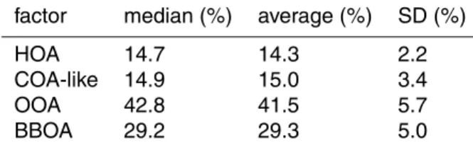
ence of alternative anchors (reference profiles). A comparison of the ME-2 source ap-portionment output of all 15 instruments resulted in relative SD from the mean between 13.7 and 22.7 % of the source’s average mass contribution depending on the factors

(HOA: 14.3±2.2 %, COA: 15.0±3.4 %, OOA: 41.5±5.7 %, BBOA: 29.3±5.0 %).

Fac-tors which tend to be subject to minor factor mixing (in this case COA) have higher

25

(4)

AMTD

8, 1559–1613, 2015

apportionment

R. Fröhlich et al.

Title Page

Tables Figures

◭ ◮

Back Close

Full Screen / Esc

Discussion

P

a

per

|

Discussion

P

a

per

|

Discussion

P

a

per

|

Discussion

P

a

per

|

1 Introduction

Measurements have shown that organic compounds constitute a major fraction of the total particulate matter (PM) all around the world (20–90 % of the submicron aerosol mass according to Kanakidou et al., 2005). Elevated concentrations of organic aerosols due to anthropogenic activities are a major contributor to the predominantly adverse

ef-5

fects of aerosols on climate (Lohmann and Feichter, 2005; Stevens and Feingold, 2009; Boucher et al., 2013; Carslaw et al., 2013), weather extremes (Wang et al., 2014a, b), Earth’s ecosystem (Mercado et al., 2009; Carslaw et al., 2010; Mahowald, 2011) or on human health (Seaton et al., 1995; Laden et al., 2000; Cohen et al., 2005; Pope and Dockery, 2006). According to recent estimates of the global burden of disease up to

10

3.6 million (Lim et al., 2013) of the about 56 million annual deaths (Mathers et al., 2005) were connected to ambient particulate air pollution in the year 2010. These numbers underline the importance of detailed knowledge about the sources of ambient aerosols

to be able to eﬃ_{ciently reduce air pollution levels.}

Positive matrix factorisation (PMF), a statistical factor analysis algorithm developed

15

by Paatero and Tapper (1994) and Paatero (1997), is a widely and successfully used approach to simplify interpretation of complex data sets by representing measurements as a linear combination of static factor profiles and their time-dependent intensities (Lanz et al., 2007, 2010; Ulbrich et al., 2009; Crippa et al., 2014). The multilinear engine implementation (ME-2, Paatero, 1999) allows for the introduction of additional

20

constraints (e.g. external factor profiles) to the algorithm. The algorithm has been heav-ily used for source identification and quantification with organic mass spectra mea-sured by the Aerodyne aerosol mass spectrometer (AMS Jayne et al., 2000; Drewnick et al., 2005; DeCarlo et al., 2006) and the related aerosol chemical speciation monitor (ACSM, Ng et al., 2011c; Fröhlich et al., 2013). Typically, the organic fraction of PM

25

(5)

AMTD

8, 1559–1613, 2015

apportionment

R. Fröhlich et al.

Title Page

Tables Figures

◭ ◮

Back Close

Full Screen / Esc

Discussion

P

a

per

|

Discussion

P

a

per

|

Discussion

P

a

per

|

Discussion

P

a

per

|

(Jimenez et al., 2009; Ng et al., 2010) remain largely unclear (Hallquist et al., 2009). Conversely, many POA sources have been identified (Zhang et al., 2011): hydrocarbon-like organic aerosol (HOA, Zhang et al., 2005a, b), biomass burning-related organic aerosol (BBOA, Alfarra et al., 2007; Aiken et al., 2010), cooking-related organic aerosol (COA, Slowik et al., 2010; Allan et al., 2010; Mohr et al., 2012; Canonaco et al., 2013;

5

Crippa et al., 2014, 2013a), coal burning-related organic aerosol (CBOA, W. W. Hu et al., 2013; Huang et al., 2014), nitrogen-enriched OA (NOA, Sun et al., 2011; Aiken et al., 2009) or local sources of primary organics (Timonen et al., 2013; Faber et al., 2013). Another marine source of secondary organic aerosol (MOA) related to MSA was reported by Crippa et al. (2013b).

10

Like every measurement or model, the results of PMF/ME-2 are subject to uncertain-ties. These uncertainties may result from the mathematical model itself (Paatero et al., 2014) or from the measurement technique applied. Within a certain measurement

tech-nique the eﬀ_{ects of basic instrument precision, e.g. calculation of the measurement}

un-certainty matrix, can be distinguished from systematic diﬀ_{erences between instruments}

15

outside of measurement precision. The latter will be investigated in this study for the first time on a large basis of 15 co-located, individual aerosol mass spectrometers

em-ploying the same experimental technique (13×Q-ACSM, 1×ToF-ACSM, 1×

HR-ToF-AMS). By comparing the source apportionment results of these 15 individual

instru-ments, previously operated at diﬀ_{erent stations all over Europe (cf. http://psi.ch/ZzWd),}

20

a measure of comparability of PMF results across data sets recorded by diﬀ_erent

in-struments is obtained.

Especially in the light of the growing number of ACSMs in Europe (promoted by the ACTRIS project: Aerosols, Clouds, and Trace gases Research InfraStructure network) and other parts of the world a better evaluation and understanding of the uncertainties

25

(6)

AMTD

8, 1559–1613, 2015

apportionment

R. Fröhlich et al.

Title Page

Tables Figures

◭ ◮

Back Close

Full Screen / Esc

Discussion

P

a

per

|

Discussion

P

a

per

|

Discussion

P

a

per

|

Discussion

P

a

per

|

2 Methodology and instrument description

The 15 Aerodyne mass spectrometers, which were provided by the co-authoring in-stitutions (see Table S1 in the Supplement) will be denoted herein as #1–#13 (Q-ACSMs), ToF (ToF-ACSM) and HR(-AMS) (HR-ToF-AMS). Overviews of wintertime aerosol sources and composition in the Paris region can be found in Crippa et al.

5

(2013a) and Bressi et al. (2014). The data sets were recorded during the ACTRIS ACSM intercomparison campaign taking place during three weeks in November and December 2013 at the SIRTA (Site Instrumental de Recherche par Télédétection Atmo-sphérique) station of the LSCE (Laboratoire des sciences du climat et l’environnement) in Gif-sur-Yvette, in the region of Paris (France). Detailed results of the intercomparison

10

can be found in part I of this study from Crenn et al. (2015). For this intercomparison study data between 16 November and 1 December were considered.

2.1 Site description

SIRTA is a well-established atmospheric observatory in the vicinity of the French megacity Paris. The measurement site is located on the plateau of Saclay on the

cam-15

pus of CEA (French Alternative Energies and Atomic Energy Commission) at “Orme

des Merisiers” (48.709◦N, 2.149◦E, 163 m a.s.l.). Being approximately 20 km

south-west of the city centre of Paris, the station is classified as regional background, sur-rounded mainly by agricultural fields, forests, small villages and other research facilities. The closest major road is located about 2 km north-east.

20

All 15 instruments were located in the same laboratory, distributed to five separate

PM_2.5 inlets on the roof of the building. A suite of additional aerosol and gas phase

instruments (e.g. Particle-Into-Liquid-Sampler coupled to an ion chromatograph (PILS-IC), proton-transfer-reaction mass spectrometer (PTR-MS), filter sampling, aethalome-ter, nephelomeaethalome-ter, scanning mobility particle sizer (SMPS), optical particle counter

25

(7)

AMTD

8, 1559–1613, 2015

apportionment

R. Fröhlich et al.

Title Page

Tables Figures

◭ ◮

Back Close

Full Screen / Esc

Discussion

P

a

per

|

Discussion

P

a

per

|

Discussion

P

a

per

|

Discussion

P

a

per

|

instruments refer to Crenn et al., 2015) were operated in parallel, providing important data facilitating the validation of sources identified in this study.

2.2 Aerosol mass spectrometers

The focus of this work lies on source apportionment performed on data recorded with

three diﬀ_{erent but related types of aerosol mass spectrometer: the high-resolution}

5

time-of-flight aerosol mass spectrometer (HR-ToF-AMS) was running alternatively in V- and W-mode every 2 min, recording aerosol spectra with a mass resolution of up

to _∆M_M =_{5000 (W-mode), the time-of-flight aerosol chemical speciation monitor}

(ToF-ACSM) operating at 10 min intervals with a resolution of _∆M_M =_{600 and the quadrupole}

aerosol chemical speciation monitor (Q-ACSM) with unit mass resolution (UMR) and

10

time steps of ∼30 min. All three instruments employ the same operational principle.

Aerosol particles are focussed into a vacuum chamber by an aerodynamic lens (Liu et al., 1995a, b, 2007; Zhang et al., 2004) where they are separated from the gas

molecules as eﬀ_{ectively as possible by a skimmer cone. These particles are flash}

va-porised on a heated (600◦C), conically shaped tungsten block. The resulting gas is

15

then ionised by electron impact (∼70 eV) and detected by the diﬀ_{erent ion mass}

spec-trometers (Tofwerk HTOF, Tofwerk ETOF, Pfeiﬀ_{er Prisma Plus QMG 220 quadrupole).}

While in the quadrupole mass spectrometer them/zchannels are scanned through at

a limited speed of typically 200 ms amu−1 (32 data points per amu), the TOF systems

measure all ions at every extraction and provide a generally greater mass-to-charge

20

resolving power and sensitivity. Vaporisation can induce thermal decomposition, while electron impact ionisation leads to extensive fragmentation. Both processes reduce the amount of available molecular information. Using fragmentation patterns known from controlled laboratory experiments (Allan et al., 2004; Aiken et al., 2008) allows for the determination of the main non-refractory aerosol species (nitrate, sulphate, ammonium,

25

chloride and bulk organic matter).

Each instrument sampled dried aerosol at a similar flow rate of∼0.1 L min−1with an

(8)

AMTD

8, 1559–1613, 2015

apportionment

R. Fröhlich et al.

Title Page

Tables Figures

◭ ◮

Back Close

Full Screen / Esc

Discussion

P

a

per

|

Discussion

P

a

per

|

Discussion

P

a

per

|

Discussion

P

a

per

|

and ACSM systems mass spectral backgrounds must be recorded and this is done dif-ferently between the two instruments. The AMS systems use a chopper slit-wheel in-side the vacuum chamber to alternate between aerosol and background measurement, the ACSM systems use an automated three way valve switch assembly. This valve is periodically switched between two lines: the air in one line was filtered (“background”)

5

while the other line carries ambient, particle laden air. All necessary calibrations

(ioni-sation eﬃ_{ciency of nitrate (IE), relative ionisation e}ﬃ_{ciencies (RIE) of ammonium and}

sulphate, mass-to-charge axis (m/z), lens alignment, volumetric flow into the vacuum

chamber, detector amplification (for more details we refer to the respective publications or the review of Canagaratna et al., 2007) were performed and monitored on site by the

10

same operators using the same calibration equipment (e.g. SMPS). Since this study is mainly focused on a relative intercomparison of the ME-2 source apportionment,

a constant collection eﬃ_{ciency of CE}=_{0.5 (Hu}ﬀ_{man et al., 2005; Matthew et al., 2008)}

was assumed for all instruments (for a more detailed analysis see Crenn et al., 2015). The following software packages were used. Q-ACSM: version 1.4.4.5. of the ACSM

15

DAQ software (Aerodyne Research Inc., Billerica, Massachusetts) during data ac-quisition and version 1.5.3.2 of the ACSM local tool (Aerodyne Research Inc., Bil-lerica, Massachusetts) for Igor Pro (Wavemetrics Inc., Lake Oswego, Oregon) for Q-ACSM data treatment and export of PMF matrices (see Supplement for discus-sion of changes in most recent software verdiscus-sion 1.5.5.0). ToF-ACSM: TOFDAQ

20

version 1.94 (TOFWERK AG, Thun, Switzerland) during acquisition and Tofware version 2.4.2 (TOFWERK AG, Thun, Switzerland) for Igor Pro for data treatment. ToF-ACSM PMF matrices were calculated manually in accordance with the proce-dures employed in the AMS software SQUIRREL v1.52G (http://cires.colorado.edu/ jimenez-group/ToFAMSResources/ToFSoftware/). AMS: standard ToF-AMS data

ac-25

(9)

AMTD

8, 1559–1613, 2015

apportionment

R. Fröhlich et al.

Title Page

Tables Figures

◭ ◮

Back Close

Full Screen / Esc

Discussion

P

a

per

|

Discussion

P

a

per

|

Discussion

P

a

per

|

Discussion

P

a

per

|

data analysis. The fragmentation table was adjusted according to recommendations (Aiken et al., 2008) in order to take into account air interferences and the water frag-mentation pattern.

2.3 Aethalometer, NOxanalyser and PTR-MS

In the context of this manuscript, data from various external measurements, namely

5

an aethalometer, a NO_x analyser and a PTR-MS were used to validate factors found

by the ME-2 source apportionment. The Magee Scientific Aethalometer model AE33 (Drinovec et al., 2014, Aerosol d.o.o., Ljubljana, Slovenia) measures black carbon (BC) aerosol by collecting aerosol on a filter and determining the light absorption at seven

diﬀ_{erent wavelengths (Hansen et al., 1984). Potential sample loading artefacts detailed}

10

in Collaud Coen et al. (2010) are automatically compensated for according to the

pro-cedures described in Drinovec et al. (2014). The absorption coeﬃ_cient_b

abs depends

on the wavelengthλand the Ångström exponentα_i, following the relationship

b_abs∝λ−αi_. ₍₁₎

By exploiting the fact that the wavelength dependence, i.e. the Ångström exponent

15

is source-specific (Sandradewi et al., 2008), the measured BC can be separated into

BC from wood burning (BC_wb) and BC from fossil fuel combustion (BCﬀ). To this end

a system of four equations has to be solved.

b_abs(λ₁)ﬀ

b_abs(λ₂)ﬀ

=

_λ

1

λ2 −αﬀ

(2)

babs(λ1)wb

b_abs(λ₂)_wb =

_λ

1

λ₂

−αwb

(3)

20

b_abs(λ₁)_tot=_b

abs(λ1)ﬀ+b_abs(λ₁)_wb (4a)

(10)

AMTD

8, 1559–1613, 2015

apportionment

R. Fröhlich et al.

Title Page

Tables Figures

◭ ◮

Back Close

Full Screen / Esc

Discussion

P

a

per

|

Discussion

P

a

per

|

Discussion

P

a

per

|

Discussion

P

a

per

|

with absorption coeﬃ_{cients of wood burning and fossil fuel combustion}_b

abs, wb/ﬀat two

diﬀ_{erent wavelengths} _λ _(here: _λ

1=470 nm and λ2=880 nm) and the corresponding

Ångström exponentsα_wb/ﬀ. According to literature α_wb typically lies between 1.9 and

2.2 (Sandradewi et al., 2008) andαﬀbetween 0.9 and 1.1 (Bond and Bergstrom, 2006).

More recent studies suggested slightly lower α_wb of 1.6–1.7 (Saleh et al., 2013; Liu

5

et al., 2014) but this does not aﬀ_{ect the overall time trends used for the correlation with}

sources found by PMF. In agreement with the sensitivity analysis done by Sciare et al.

(2011) for the Paris region, Ångström exponents ofα_wb=_{2 and}_α_ﬀ=_{1 were used in the}

BC source apportionment of this study. The fractions of BC emitted by the respective sources can then be calculated linearly from the total measured BC and the fraction of

10

the corresponding absorption coeﬃ_cient.

NO_x concentrations were measured by a photolytic NO-NO₂ analyser (model

T200UP NO-NO₂, Teledyne API, San Diego, CA, USA) via ozone-induced

chemilumi-nescence. Gaseous methanol and acetonitrile concentrations were detected by proton-transfer-reaction mass spectrometry (PTR-MS, serial # 10-HS02 079, Ionicon Analytik,

15

Innsbruck, Austria, Hansel et al., 1995; Graus et al., 2010) which is described else-where (Sciare et al., 2011).

2.4 ME-2 and SoFi tool

For source apportionment (SA) of organic aerosol mass spectral data sets the methods of choice usually are two-dimensional bilinear models like PMF (Paatero and Tapper,

20

1994; Paatero, 1997) or chemical mass balance (CMB, Watson et al., 1997; Ng et al., 2011b). Especially PMF has successfully been used in numerous AMS SA studies

(Zhang et al., 2011). In both methods the organicm×nspectral matrix X, containing

morganic mass spectra (rows) with nion fragments each (columns), is factorised into

two submatrices, the profilesFand time seriesG.Fis ap×nandGam×pmatrix with

25

pindicating the number of profiles. The residualm×nmatrixEcontains the fraction of

(11)

AMTD

8, 1559–1613, 2015

apportionment

R. Fröhlich et al.

Title Page

Tables Figures

◭ ◮

Back Close

Full Screen / Esc

Discussion

P

a

per

|

Discussion

P

a

per

|

Discussion

P

a

per

|

Discussion

P

a

per

|

by the PMF algorithm.

X=_GF+_E ₍₅₎

Within the ME-2 package several cases of PMF are implemented: the traditional un-constrained PMF, PMF with controlled rotations (in many cases this is simply denoted “ME-2”), or fully constrained PMF (a form of CMB). While in unconstrained PMF the

5

algorithm models the (entirely positive) profile and time series matricesFand Gwith

a pre-set number of factorspby iteratively minimising the quantityQ(main part of the

object function as defined by Paatero and Hopke, 2009), the fully constrained (CMB-like) PMF algorithm needs well defined factor profiles as input and attributes a time series of concentrations to them.

10

Q=

m X

i=₁ n X

j=₁

e

i j

σi j 2

(6)

withe_{i j} being the elements of the residual matrix Eand σ_{i j} the measurement

uncer-tainties of ion fragmentj at time step i. In many cases, e.g. when two factors have

similar time series (e.g. heating and cooking in the evening) or profiles (e.g. traﬃ_{c and}

cooking, Mohr et al., 2009) the totally unconstrained PMF has diﬃ_{culties separating}

15

these factors (this was already pointed out in former studies, e.g. by Sun et al., 2010). The multilinear engine (ME-2) provides additional control over the rotational ambiguity (Paatero and Hopke, 2009). Here the solution space is explored by introducing a

pri-ori information (e.g. factor profiles) for some (not necessary all) of the factors p. The

strength of this additional constraint is set by the so-calledavalue (Paatero and Hopke,

20

2009; Brown et al., 2012), which determines how much deviation from the constraint profile the model allows. It ranges from zero to one and can be understood as the

relative fraction how much eachm/z may individually deviate from the a priori profile

(Canonaco et al., 2013). That way ME-2 covers the whole range of bilinear models

from fully constrained (a=_{0) to completely unconstrained PMF (no}_a_{value set).}

(12)

AMTD

8, 1559–1613, 2015

apportionment

R. Fröhlich et al.

Title Page

Tables Figures

◭ ◮

Back Close

Full Screen / Esc

Discussion

P

a

per

|

Discussion

P

a

per

|

Discussion

P

a

per

|

Discussion

P

a

per

|

ing away from the unconstrained solution typically leads to an increase inQ. The

mag-nitude of this increase ofQ is used in order to remove solutions whose rotations are

not a mathematically adequate representation of the input dataset. All factor analyses presented in this study were performed in the robust mode (Paatero, 1997).

Initialisation of the ME-2 engine and analysis of the results was performed using the

5

source finder tool (SoFi v4.6, http://psi.ch/HGdP, Canonaco et al., 2013) package for Igor Pro (WaveMetrics Inc., Lake Oswego, Oregon).

2.5 Model input and data preparation

As an input, the ME-2 algorithm requires the organic data matrix, the associated error

matrix, and the corresponding time and mass-to-charge (m/z) axis. For each

instru-10

ment the input data was created up tom/z100 and individually cleaned up. Bad data

points were identified by standard diagnostics (airbeam signal, inlet pressure, voltage

settings, etc.). A uniform CE=_{0.5 and a uniform organics RIE}

org=1.4 were used for

all data sets. The corresponding ionisation eﬃ_{ciency (IE) or, more accurately for the}

Q-ACSMs, the response factor (RF) calibration values were determined during the first

15

week of the intercomparison study on site (Crenn et al., 2015) and can be found in

Table S2. Q-ACSM data was corrected for a decrease in ion transmission at highm/z

(&55) according to a standard curve obtained by Ng et al. (2011c). For further dis-cussion and recent software updates concerning the RIT calculation for PMF matrices refer to the discussion in the Supplement. To correct for the decay of the detector

am-20

plification the airbeam N₂ signal at m/z 28 was used (reference value: 1×10−7A)

maintaining the detectors at gain values of around 20 000.

The ToF-ACSM data set exhibited an unusual (exponentially decaying) drift in addi-tion to the drift of the airbeam signals, visible in the always present background signals like the one of stable tungsten isotopes (originating from the ioniser filament). From

25

the largest signals in the background (m/z 105, 130, 132, 182 and 221) a correction

function was deduced and applied to the data set. This drift is attributed to transient

(13)

AMTD

8, 1559–1613, 2015

apportionment

R. Fröhlich et al.

Title Page

Tables Figures

◭ ◮

Back Close

Full Screen / Esc

Discussion

P

a

per

|

Discussion

P

a

per

|

Discussion

P

a

per

|

Discussion

P

a

per

|

A probably too short delay time of the quadrupole scan after a valve switch (125 ms)

caused physically not meaningful negative values at the signal channel of m/z 12,

therefore the m/z 12 column was removed from all Q-ACSM matrices prior to PMF

analysis.m/zchannels with weak signals may influence the operation of the PMF

al-gorithm and therefore also the solutions in a suboptimal way because the alal-gorithm

5

may try to apportion nonsensical noise. In order to avoid this the corresponding uncer-tainty of weak channels can be increased to reduce their weight according to Eq. (6).

Table S3 shows a list of down-weightedm/zchannels for each instrument. The

deci-sion if a channel is down-weighted or not was made individually either because of low signal-to-noise ratio according to the recommendations of Ulbrich et al. (2009) or

be-10

cause of spotted outliers with high weighted residuals. Furthermore, the uncertainties

ofm/zchannels which are not directly measured but recalculated from fractions of the

signal atm/z 44 via the fragmentation table (Allan et al., 2004) are adjusted as well

according to the recommendation of Ulbrich et al. (2009).

3 Results

15

In the discussion below the 13 participating Q-ACSMs in this study are denoted “#1” to “#13” while the ToF-ACSM will be denoted “ToF” and the HR-ToF-AMS “HR”, following the notation of the companion paper of Crenn et al. (2015). A complete list of the participating instruments can be found in Table S1. Times are presented in local time

(CET=_UTC+_{1 h).}

20

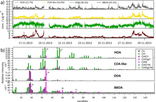
3.1 Organic time series

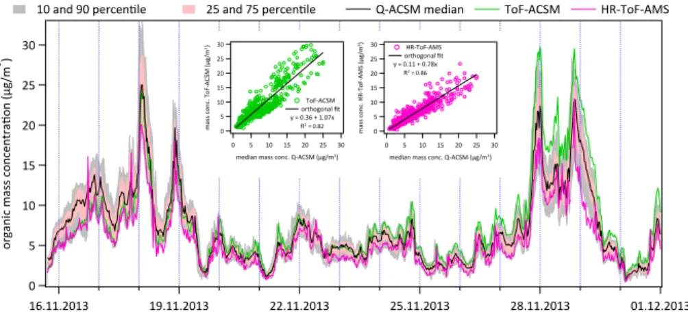
Figure 1 shows the time traces of bulk organic matter during the sixteen days of simul-taneous measurement used for the subsequent ME-2 analysis (16 November 2013 to 1 December 2013, this corresponds to 550–780 data points depending on data avail-ability of each instrument). The median organic concentration of the 13 Q-ACSMs is

(14)

AMTD

8, 1559–1613, 2015

apportionment

R. Fröhlich et al.

Title Page

Tables Figures

◭ ◮

Back Close

Full Screen / Esc

Discussion

P

a

per

|

Discussion

P

a

per

|

Discussion

P

a

per

|

Discussion

P

a

per

|

displayed as black line with the interquartile range (IQR) (25–75 percentile) shaded in red and the 10–90 percentile range shaded in grey. The corrected ToF-ACSM time series is shown in green and the AMS in pink. Correlations of ToF-ACSM and AMS with the median of the Q-ACSMs is shown in the two inset graphs. Good qual-itative and quantqual-itative agreement between all 15 aerosol mass spectrometers was

5

achieved (R2=_{0.82–0.99, slope}=_{0.70–1.37, see Crenn et al. (2015) for}

intercompar-ison between Q-ACSMs or Fig. 1 for comparintercompar-ison of Q-ACSMs to HR-AMS and

ToF-ACSM). Average organic matter concentrations during the whole period with 6.9 µg m−3

(range≈0.7–25 µg m−3) were in the range of typical OA concentrations at this site

(Pe-tit et al., 2014), providing good boundary conditions (high signal-to-noise and

variabil-10

ity) for PMF source apportionment. For a more detailed analysis of the concentration ranges we refer to Crenn et al. (2015).

3.2 Organic mass spectra

The mass spectrometer discriminates molecular fragments of certain mass-to-charge ratios resulting in the typical stick plot representation of mass spectra. The bulk organic

15

signal is calculated from the sum of the sticks (total integrated signal for a given integer

m/z) associated with organic molecules or molecular fragments according to known

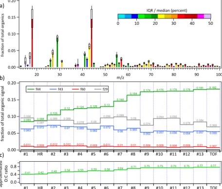
fragmentation patterns detailed in Allan et al. (2004). This is done under the assump-tion that with constant boundary condiassump-tions the fragmentaassump-tion is constant as well. The sticks in Fig. 2a represent the median fractions of total organic matter at the respective

20

mass-to-charge ratios for the 13 Q-ACSM instruments during an interruption-free 20 h

period (26 November 10:00–27 November 06:00 local time (UTC+_{1)). The IQR and}

the full range are displayed as boxes and whiskers respectively.

There is significant information remaining in the organic molecular fragments. For

example fragments atm/z60 (mainly C₂H₄O+₂) andm/z73 (C₃H₅O+₂) mostly originate

25

from primary biomass burning particles (Alfarra et al., 2007; Ng et al., 2010; Cubison

et al., 2011), there are exceptions in marine environments where the signal atm/z60

(15)

AMTD

8, 1559–1613, 2015

apportionment

R. Fröhlich et al.

Title Page

Tables Figures

◭ ◮

Back Close

Full Screen / Esc

Discussion

P

a

per

|

Discussion

P

a

per

|

Discussion

P

a

per

|

Discussion

P

a

per

|

as well is often enhanced in wood burning emissions but is also observed from other

sources e.g. SOA (Chhabra et al., 2010). The fragments atm/z 43 (mainly C₂H₃O+)

andm/z 44 (mainly CO+₂) can help retrieving information about ageing and oxidation

state of secondary organic aerosol (SOA) (Ng et al., 2010, 2011a).

The four fragments mentioned above are shown in Fig. 2b as fraction of the total

5

organic signal for all 15 participating instruments during the 20 h period mentioned above. As already represented in the colour bar of Fig. 2a it is evident that while most fragments have more or less similar contributions to total organic matter (e.g. f29, f43 and f60 in Fig. 2b), there is significant instrument-to-instrument variation of the f44.

It is to note that the organic signals at m/z 16, 17 and 18 are also calculated from

10

m/z44 according to the fragmentation patterns highlighting the importance of the f44

variations (cf Fig. 2a). A comparison of the mass spectra after the stick atm/z44 and

all related peaks were removed shows very similar relative spectra (IQR/median<20 %

for mostm/z, cf. Fig. S1 in the Supplement). Onlym/z29 which is mostly CHO+ still

shows a small increase (see Fig. S1b). This may either indicate a connection tom/z

15

44 (CO+₂) or a small influence of air interferences.

Figure 2c shows that estimated O : C ratios based on f44 (Aiken et al., 2008) in this study varied from 0.41 to 0.77 for the same ambient aerosol. An elemental analysis of the HR-AMS data, however yielded an O : C ratio of 0.38. This is close to the O : C ratio calculated from the formula of Aiken et al. (2008) for the HR-AMS spectrum (0.42).

20

The consistency of the HR-AMS elemental analysis was confirmed by comparison to a known organic mixture beforehand. As a consequence the “real” O : C value during the intercomparison campaign most likely lies at the low end of Fig. 2c and the ACSMs overestimate O : C.

The fraction of m/z 44 to total organic matter measured (f44) continuously varies

25

compared to the mean between factors of 0.6 and 1.3 (from 8.5 and 18.2 %, Fig. 2b).

Although the absolute value of f44 that is measured by diﬀ_{erent instruments is}

(16)

con-AMTD

8, 1559–1613, 2015

apportionment

R. Fröhlich et al.

Title Page

Tables Figures

◭ ◮

Back Close

Full Screen / Esc

Discussion

P

a

per

|

Discussion

P

a

per

|

Discussion

P

a

per

|

Discussion

P

a

per

|

stant over time and does not vary with aerosol composition (see Fig. S2). Moreover, the precision of an individual, stable instrument is good and relative changes observed for any given instrument can be unambiguously interpreted. Thus, source

apportion-ment analyses are not compromised, and indeed are only slightly aﬀ_{ected as discussed}

hereafter.

5

Measurements of organic standards could be used to calibrate and allow for the

intercomparison of the absolute f44 values observed in diﬀ_{erent ACSM instruments.}

However, in the absence of these calibrations, caution should be exercised in

quanti-tatively comparing f44 values obtained by diﬀ_{erent ACSM instruments. This includes}

application of the f44 vs. f43 “triangle plot” (Ng et al., 2010) that is widely used to

10

describe oxygenated organic aerosol (OOA) factors and comparisons of O : C values derived from ACSM f44 values.

A direct influence of the vaporiser temperature on this variability is ruled out by ACSM measurements of ambient reference aerosols (nebulisation of filter extracts, see

Däl-lenbach et al., 2015, for method description) at diﬀ_{erent vaporiser temperatures.}

Rela-15

tive organic spectra remained constant over a wide range of temperatures (see Fig. S3 and caption) as it was already shown for several organic standards by Canagaratna et al. (2015). Also the fragmentation of inorganic molecules remained constant over

a range of at least 550±70◦C.

The f44 variability is observed to be larger in the ACSM instruments than the AMS

20

instruments (Ng et al., 2011c; Canagaratna et al., 2007). The ACSM and AMS in-struments are based on the same particle vaporisation and ionisation schemes

(us-ing the identical particle vaporiser), but they are operated with diﬀ_{erent open/closed}

or open/filter switching cycles required for background subtraction. AMS instruments

are typically operated with a faster switching cycle (<5 s) than the Q-ACSMs (∼30 s),

25

which in turn have shorter open times than the ToF-ACSM with the “fast-mode MS” (Kimmel et al., 2011) setting employed in this campaign (480 s open/120 s closed). Is is noted that a fast filter switching scheme analogous to that of the Q-ACSM has

(17)

AMTD

8, 1559–1613, 2015

apportionment

R. Fröhlich et al.

Title Page

Tables Figures

◭ ◮

Back Close

Full Screen / Esc

Discussion

P

a

per

|

Discussion

P

a

per

|

Discussion

P

a

per

|

Discussion

P

a

per

|

diﬀ_{erent degrees of sensitivity to delayed vaporisation and pyrolysis artefacts. E}ﬀ_orts

to understand and diminish the variability in f44 measured by ACSM instruments are ongoing.

3.3 HR-ToF-AMS source apportionment

Several publications have demonstrated that higher time andm/z-resolution provided

5

by the HR-ToF-AMS in contrast to the UMR of the ACSM result in less rotational am-biguity and provide superior source resolution (Aiken et al., 2009; Zhang et al., 2011). Therefore, we first perform a PMF of the HR-ToF-AMS data to determine the likely re-solvable factors and their characteristics. High-resolution analysis was performed up to

a mass-to-charge ratio of 130 resulting in 355 diﬀ_{erent organic fragments.}

10

Completely unconstrained PMF analysis yields four factors: hydrocarbon-like organic aerosol (HOA), cooking-like organic aerosol (COA), oxygenated organic aerosol (OOA) and biomass burning related aerosol (BBOA). Higher numbers of factors result in ran-dom splitting of already identified factors. However, in the four factor solution, the HOA and COA factors show signs of source mixing (mainly with the wood burning related

15

source), like unusually high f44. An extension of the analysis up to eight factors leads to an unmixing of the two factors. Therefore, these clearly resolved HOA and COA factor profiles from the 8-factor solution were extracted, saved and used as anchors

in a subsequent four factor ME-2 analysis with tight constraints ofa=_{0.1 each. The}

other two factors remained unconstrained. This approach resulted in better correlations

20

with external tracers for all factors than the completely unconstrained four factor solu-tion. A similar approach of increasing the number of factors in unconstrained PMF and subsequent combination of duplicate factors was used in previous studies (Docherty et al., 2011; Li et al., 2015). The resulting time series and factor profiles are shown in Fig. 3a and b.

25

(18)

ex-AMTD

8, 1559–1613, 2015

apportionment

R. Fröhlich et al.

Title Page

Tables Figures

◭ ◮

Back Close

Full Screen / Esc

Discussion

P

a

per

|

Discussion

P

a

per

|

Discussion

P

a

per

|

Discussion

P

a

per

|

plained below (see Fig. S4a–d and Table S4) and by identification of diurnal emission patterns (see Fig. 4).

Factor #1 (HOA) is dominated by ions related to aliphatic hydrocarbons, e.g. atm/z

41 (C₃H+₅),m/z43 (C₃H+₇),m/z 55 (C₄H₇+),m/z57 (C₄H+₉),m/z67 (C₅H+₇),m/z69

(C₅H+₉),m/z71 (C₅H+₁₁),m/z79 (C₆H+₇),m/z81 (C₆H+₉) andm/z83 (C₆H+₁₁) (Zhang

5

et al., 2005b). HOA typically is emitted by combustion of (hydrocarbon-rich) fossil fuel, e.g. from motor vehicles. The diurnal variation (Fig. 4) shows two clear peaks during

morning and evening rush hours and the time series correlates well with ambient NO_x

(R2=_{0.65) concentrations and the fossil fuel-related fraction of BC retrieved from the}

aethalometer (R2=_0.68).

10

The mass spectrum of factor #2, identified as organic aerosol related to cooking activities, shows similarities to the HOA with highest contributions of peaks at similar

mass-to-charge ratios (m/z 27, 41, 43, 55, 57, 67, 69, 79, 81, 83) but with a higher

contribution of oxygenated species at m/z 41 (C₂HO+), m/z 43 (C₂H₃O+), m/z 55

(C₃H₃O+),m/z57 (C₃H₅O+),m/z69 (C₄H₅O+),m/z71 (C₄H₇O+),m/z81 (C₅H₅O+)

15

andm/z83 (C₅H₇O+). This is in accordance with previous publications (Slowik et al.,

2010; Allan et al., 2010; Mohr et al., 2012; Canonaco et al., 2013; Crippa et al., 2013a,

2014). Especially the oxygenated fragment atm/z 55 can serve as a good indicator

for COA. C₃H₃O+ is plotted together with the COA factor in Fig. S4b. Its correlation to

COA (R2=_{0.80) is much higher than to HOA (}_R2=_{0.38). Also C}

6H10O +

which was

20

identified as a marker for COA before by Sun et al. (2011) and Crippa et al. (2013b)

correlates better with the COA factor (R2=_{0.38) than with the HOA factor (}_R2=_0.23,

see grey trace in Fig. S4b). Typical for COA aerosol are the distinctively diﬀ_erent

(com-pared to the HOA factor) ratios betweenm/z41 and 43, betweenm/z55 and 57 and

betweenm/z 69 and 71 (Mohr et al., 2012; Crippa et al., 2013a). In Fig. S5 the COA

25

(19)

AMTD

8, 1559–1613, 2015

apportionment

R. Fröhlich et al.

Title Page

Tables Figures

◭ ◮

Back Close

Full Screen / Esc

Discussion

P

a

per

|

Discussion

P

a

per

|

Discussion

P

a

per

|

Discussion

P

a

per

|

time in the diurnal variation (Fig. 4) are characteristic of clearly resolved COA factors in previous studies and support the present interpretation.

The secondary factor #3 consists of highly oxidised (high f44) organic aerosol (OOA). The diurnal cycle is more or less flat and the overall concentrations are more driven by meteorology than by emissions (see OOA time trace in Fig. 3a). This is supported by

5

the stronger correlation of OOA to sulphate (R2=_{0.43), ammonium (}_R2=_{0.54), and}

nitrate (R2=_{0.47, see Fig. S4d) than for the other three factors (cf. Table S4). As is}

frequently the case for winter campaigns, the OOA could not be further separated into oxygenation/volatility-dependent fractions (Lanz et al., 2010; Zhang et al., 2011).

The most descriptive features in the mass spectrum of factor #4 identifying it as

10

BBOA are the oxygenated peaks at m/z 60 (C₂H₄O+₂) andm/z 73 (C₃H₅O+₂). They

are associated with fragmentation of levoglucosan which is produced in the devolatil-isation of cellulose making it a good tracer for biomass burning emissions (Simoneit

et al., 1999; Q. H. Hu et al., 2013). Generally BBOA profiles from diﬀ_erent

measure-ment sites are less uniform than e.g. HOA profiles because of the higher variability of

15

fuel and burning conditions (Weimer et al., 2008; Grieshop et al., 2009; Heringa et al., 2011, 2012; Crippa et al., 2014). The BBOA factor profiles from this study contain relatively high f44 which may be an indication of ageing and oxidation prior to detec-tion. Similar BBOA spectra were observed before, e.g. in winter in Paris (Crippa et al., 2013a) and in Zurich (Canonaco et al., 2013). The diurnal variation shows a steep

20

increase in the afternoon and evening and a subsequent decrease after midnight, cor-responding with domestic heating habits. In Fig. S4c the BBOA factor shows very good

correlation with BC_wb from the aethalometer (R2=_{0.90) and good correlation to}

gas-phase methanol (R2=_{0.76) and acetonitrile (}_R2=_{0.48) measured with a PTR-MS. In}

winter wood combustion is a significant source for primary and secondary methanol

25

(20)

AMTD

8, 1559–1613, 2015

apportionment

R. Fröhlich et al.

Title Page

Tables Figures

◭ ◮

Back Close

Full Screen / Esc

Discussion

P

a

per

|

Discussion

P

a

per

|

Discussion

P

a

per

|

Discussion

P

a

per

|

factors as well as the fingerprint of factor profiles are in good agreement with results of Crippa et al. (2013a) from winter 2010 at a nearby site.

The amount of factors (four) found in this HR-PMF analysis provides the basis for the analysis of the parallel unit mass resolution (UMR) data sets from the further 13

Q-ACSMs and the 1 ToF-ACSM. The resolving power of the ToF-ACSM is suﬃ_cient

5

to resolve a subset of the ions used in the HR-PMF analysis described here (Fröhlich et al., 2013). However, the uncertainties associated for inclusion in an HR-PMF study using the ToF-ACSM data are still undetermined. Therefore only UMR analyses of the ToF-ACSM data were performed for this intercomparison study.

3.4 ACSM (UMR) source apportionment

10

PMF analyses were performed individually on all 14 ACSM data sets. The data prepa-ration procedures were described in Sect. 2.5 and Table S3. For most instruments, a pure PMF analysis (no additional constraints on any of the factor profiles) could only resolve three separate factors (HOA, BBOA, OOA). The three factor solutions showed larger instrument-to-instrument variability and less correlation to external

measure-15

ments for most ACSMs (especially of the HOA factor) than the four factor ME-2 so-lutions presented hereafter. Contributions and correlations of the three factor PMF can be found in Fig. S6 and Table S5.

Based on the HR-PMF analysis presented in Sect. 3.3 a COA factor was introduced

with a variableavalue. A verified anchor spectrum from a previous study at the nearby

20

measurement site SIRTA zone 1 of Crippa et al. (2013a) was used (reference

spec-tra from Crippa et al. (2013a) are labelled with the subscript _Paris in the following).

The HOA factor, if possible, remained unconstrained or was extracted from a previ-ous PMF solution with a higher number of factors similar to the retrieval of the COA factor in the HR-PMF in Sect. 3.3. HOA reference profiles retrieved this way are

in-25

dividual for each instrument and denoted HOA_indv in the following. The two additional

(21)

al-AMTD

8, 1559–1613, 2015

apportionment

R. Fröhlich et al.

Title Page

Tables Figures

◭ ◮

Back Close

Full Screen / Esc

Discussion

P

a

per

|

Discussion

P

a

per

|

Discussion

P

a

per

|

Discussion

P

a

per

|

ways possible and a more common approach is the adaptation of reference spectra from a database of previous experiments. Therefore the ME-2 results acquired with

the use of the database profiles HOA_Paris and COA_Paris are shown as well for

com-parison. The influence of an alternative anchor (see Fig. 7, top panel, and Sect. 3.5.3) proved to be only marginal. The source apportionment of the ToF-ACSM data produces

5

clearer diurnal trends due to less scatter in the time series and higher temporal resolu-tion compared to the Q-ACSM data. This facilitates source identificaresolu-tion. In this study, however, for a clear separation of all four factors without the extra information of HR fitted spectra, the additional controls (e.g. possibility to introduce anchor spectra) of the ME-2 package were necessary for the source apportionment of both, ToF-ACSM and

10

Q-ACSM data.

Optimal a values in each case were determined by systematic variation of the a

value in relation to increases or decreases of the correlation coeﬃ_cient_R2 _{of the}

fac-tor time series with external tracers. The correlations which were maximised for the

determination of the besta values were: BBOA factor with BC_wb, OOA factor with

in-15

organic SO₄and HOA factor with BCﬀ and NOx. Correlation maxima (R2) are listed in

Table 2. Changes inavalue usually aﬀ_{ected mainly the correlations of the HOA factor}

while the correlations of the BBOA and OOA factors were quite stable. On that account

two correlations to HOA were made. The sum of the two HOAR2 is maximised. For

COA no reliable external tracer was measured. For all factors good correlations with

20

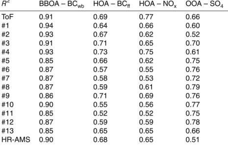
the respective external measurement were reached: BBOA – BC_wb: medianR2=_0.87

(range 0.85–0.94), HOA – BCﬀ: medianR

2₌

0.65 (range 0.52–0.73), HOA – NO_x:

me-dianR2=_{0.62 (range 0.52–0.77), OOA – SO}

4: median 0.72 (range 0.51–0.79).

The applied strategy was: increase of a in steps of ∆_a=_{0.05 until a maximum} _R2

(coeﬃ_{cient of correlation between time series of resulting factors and corresponding}

25

external tracers) is found. If more than one factor profile is constrained, first both a

values are varied simultaneously until a maximumR2 is found. From this point, thea

(22)

AMTD

8, 1559–1613, 2015

apportionment

R. Fröhlich et al.

Title Page

Tables Figures

◭ ◮

Back Close

Full Screen / Esc

Discussion

P

a

per

|

Discussion

P

a

per

|

Discussion

P

a

per

|

Discussion

P

a

per

|

stays constant. This way a large range ofa values could be explored for each

instru-ment.

It is to note that of course also the BC source apportionment and other external data used for this sensitivity analysis are prone to uncertainties. The approach de-tailed above therefore should, if applied elsewhere, always be used with caution. In the

5

presented case the optimisation ofa values also assured the comparability of the 15

solutions used for the intercomparison of the ME-2 method. A thorough discussion of the uncertainties of the BC source apportionment method and a comparison to other source apportionment methods can be found in Favez et al. (2010).

Optimisedavalues for each instrument are shown in Table 1. In some cases no clear

10

maximum of the temporal correlation to external tracers but a plateau of the

correla-tion coeﬃ_cient_R2 _{could be found and the largest possible}_a_{value is noted in Table 1.}

This indicates a stable HOA factor. The COA factor which could not be resolved in the pure PMF of the ACSM data sets is less stable and therefore generally needs a tighter

constraint, i.e. a loweravalue (see right column of Table 1). This is necessary to avoid

15

as much as possible potential mixing of COA and BBOA factors. Similar diurnal cycles of heating and cooking activities (both sources have the highest emissions during the evening hours) pose a risk for factor mixing especially in the Q-ACSM data sets which have lower mass resolution and generally less precision. Two weeks of Q-ACSM

mea-surement result in about 700 mass spectra of which only∼30 are including lunchtime

20

COA emissions and the emission peak of COA aerosol in the evening overlaps with wood burning emissions. In addition COA emissions may be significantly lower and partly transported in contrast to measurements at an urban site. All this may put COA at the edge of ME-2 resolvability. Due to this the Q-ACSM COA factor may still contain some mixed-in BBOA fraction or the other way round. Also the fact that the contribution

25

(23)

AMTD

8, 1559–1613, 2015

apportionment

R. Fröhlich et al.

Title Page

Tables Figures

◭ ◮

Back Close

Full Screen / Esc

Discussion

P

a

per

|

Discussion

P

a

per

|

Discussion

P

a

per

|

Discussion

P

a

per

|

to the first two points, real COA emissions may be somewhat lower than indicated by

the COA factor and the factor is named COA-like in the following. For HOA_indva smaller

range ofavalues (a=_0.01–0.10;∆_a=_{0.01) was explored to maintain similarity to the}

extracted profiles.

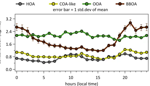
3.5 Intercomparison of source apportionment results

5

3.5.1 Time series

Diurnal variation and factor profiles of all 15 solutions (13×Q-ACSM, 1×ToF-ACSM,

1×HR-ToF-AMS) are displayed in Fig. 5 (for full time series see Fig. S7) and Figs. S13

and S14. To avoid influence of a potentially varying CE, the diurnal plots show the relative fractions of the total apportioned organic matter for the respective source

fac-10

tors instead of absolute concentrations. The diurnal variation plots of the four factors show the median of all Q-ACSMs (black) and the IQR as well as the 10–90 percentile range together with the diurnal variation of AMS (pink) and ToF-ACSM (green) fac-tors. To facilitate comparison and to avoid a too large influence of the drift observed in the ToF-ACSM (see Sect. 2.5), all diurnal time traces (Q-ACSMs, HR-ToF-AMS and

15

ToF-ACSM) were calculated only for the measurement period between 20 November and 2 December, discarding the first four days of measurement in which the observed exponentially decaying drift had the largest influence. Morning and evening rush hour peaks in the HOA as well as lunch and dinner time peaks in the COA-like factor are easily discernible around 1 p.m. and 9 p.m. The fraction of BBOA significantly increases

20

in the evening when domestic heating activities are highest and decreases again after midnight with a small plateau in the morning when people are waking up. The apparent decrease of the OOA relative contribution in the evening can be attributed to the in-crease of BBOA since the absolute concentrations of OOA show no diurnal trends (cf. Fig. S7). The observed trend of the diurnal variations are similar in all 15 instruments.

25

(24)

se-AMTD

8, 1559–1613, 2015

apportionment

R. Fröhlich et al.

Title Page

Tables Figures

◭ ◮

Back Close

Full Screen / Esc

Discussion

P

a

per

|

Discussion

P

a

per

|

Discussion

P

a

per

|

Discussion

P

a

per

|

ries to the median of all instruments are illustrated in the Supplement in Figs. S8–S11. Slopes range between 0.73–1.27 (HOA), 0.62–1.43 (COA-like), 0.77–1.23 (BBOA) and

0.66–1.28 (OOA) with correlation coeﬃ_cients_R2_{between 0.63–0.94 (HOA, median}_R2_:

0.91), 0.55–0.91 (COA-like, medianR2: 0.85), 0.90–0.98 (BBOA, medianR2: 0.95) and

0.72–0.95 (OOA, medianR2: 0.91).

5

Diurnal variation of the relative factor contributions from the HR-AMS and the ToF-ACSM data sets are largely within the range of the Q-ToF-ACSMs. The morning peak of the

HOA is slightly smaller in the HR-AMS than in the other devices (morning traﬃ_{c peak}

contributions: 22.5 % (HR-AMS), 27.7 % (median Q-ACSMs), 30.4 % (ToF-ACSM)) and the source apportionment of the ToF-ACSM data set yielded slightly lower OOA but

10

higher BBOA concentrations (cf. Fig. 7, bottom panel). It is noted that the non-uniform time steps the Q-ACSM data is recorded at, and several unplanned measurement in-terruptions of some of the instruments made it impossible to completely synchronise all devices. This contributes an unknown, likely small fraction of the total uncertainty.

The lower panel of Fig. 5 shows the diurnal variation of the model residuals scaled

15

to the total organic concentrations. Residuals of ToF-ACSM and Q-ACSMs fluctuate

around zero and are always within a range smaller than±2 % of total organic

concen-trations. In the evening hours when total organic concentrations are highest the scaled residuals tend to be slightly larger. The HR-AMS residuals, however, are higher and

purely positive. A more detailed analysis shows that allm/z channels are aﬀ_{ected to}

20

a similar extent. The reason for the purely positive residuals is unknown, but no signifi-cant temporal variation and no signifisignifi-cant change or decrease of the residuals even in

PMF runs with high number of factors (>10) indicate that the residuals are not

con-nected with additional factors missing in the current analysis.

3.5.2 Profiles

25

(25)

AMTD

8, 1559–1613, 2015

apportionment

R. Fröhlich et al.

Title Page

Tables Figures

◭ ◮

Back Close

Full Screen / Esc

Discussion

P

a

per

|

Discussion

P

a

per

|

Discussion

P

a

per

|

Discussion

P

a

per

|

box relative to the median. For the BBOA and OOA factors them/zrange between 50

and 100 is enlarged in separate insets. The typical features of each factor are similar to the HR data in Sect. 3.3.

The aliphatic hydrocarbon signals characteristic for HOA have relatively stable

contri-butions to the HOA source spectrum (box/15 %, green colour) in all instruments. The

5

variation ofm/z43 is slightly higher (≈25 %, yellow) and the mass-to-charge ratios 29

and 44 (and 16–18 which are calculated directly fromm/z44, see Allan et al., 2004)

have quite large boxes (>50 %, violet). These fragments are also partly apportioned

to BBOA and OOA which could indicate a minor mixing of these sources into the HOA factor for some instruments. Considering the full range (whiskers) instrument #13 (see

10

Fig. S13) represents an outlier with highm/z 44 in the HOA. It is noted that in most

ME-2 source apportionments this solution would have been discarded and an approach with a constrained externally measured HOA profile would have been favoured (similar to the approach used to calculate the second bars from the left in Fig. 7, top panel). For the sake of comparability the solution with the individually extracted HOA profile of

15

instrument #13 is still included in this analysis. Other contributingm/zchannels which

exhibit a larger variability of more than 30 % in the HOA profiles are 26, 27, 53, 66, 77 and 91.

The second panel of Fig. 6 shows the variation of the COA source profiles which

were constrained with lowavalues. It is noted that the method of adding constraints to

20

the ME-2 output naturally has an eﬀ_{ect on its maximum possible variability. Therefore}

no variations'20 % are observed.

The BBOA profile is shown in the third panel. The variations of the important markers

atm/z29, 60 and 73 show the smallest variations (/25 %). The f44 however exhibits

a variability of≈50 %. A more detailed look at the BBOA profiles in Fig. S14 shows

25

(26)

AMTD

8, 1559–1613, 2015

apportionment

R. Fröhlich et al.

Title Page

Tables Figures

◭ ◮

Back Close

Full Screen / Esc

Discussion

P

a

per

|

Discussion

P

a

per

|

Discussion

P

a

per

|

Discussion

P

a

per

|

f44 to characterise ageing of biomass burning plumes (as it could be shown for AMS data by Cubison et al., 2011) from ACSM datasets.

The OOA factor profile shows only slightly smaller absolute variation (size of box) of f44 as the BBOA profile, but since here f44 is larger in general, the resulting size of

the box in relation to the median is only on the order of≈20 %. Considering the full

5

range f44 varies by about 40 %, similar to the variation of f44 in the input organic mass spectra. Again, a look at Fig. S14 reveals an increasing f44 in the OOA source profile

with increasing total f44. There are only few additionalm/zchannels having significant

contributions to OOA. The magnification of the region abovem/z 50 shows only very

low signals with high variations which predominantly can be considered noise.

10

The fact that the f44 has a high instrument-to-instrument variability in all uncon-strained factors has important implications for the application of reference profiles

mea-sured with an AMS or another ACSM to ACSM data sets. Constraints onm/z44 should

be avoided or loosened as much as possible. Alternatively the f44 in such reference profiles should be subjected to a sensitivity test (e.g. by manually changing the f44 of

15

a reference profile).

The source profiles of the ME-2 analysis of the ToF-ACSM data set are shown in Fig. S12 together with box and whisker plots of the Q-ACSM profiles. Generally the ACSM source profiles lie well within the range of the Q-ACSMs. Since the ToF-ACSM had the highest f44 of all instruments all factor profiles lie at the upper end of

20

the Q-ACSM f44 range. The signals at higher mass-to-charge ratios are a bit smaller. This could either be due to an overestimation of the relative ion transmission (RIT) correction performed on the Q-ACSM mass spectral data (see RIT discussion in the Supplement) or to loss of smaller signals in the ToF-ACSM caused by the operational issue with the detector amplification detailed in Sect. 2.5. The latter is unlikely but

25