www.adv-stat-clim-meteorol-oceanogr.net/2/137/2016/ doi:10.5194/ascmo-2-137-2016
© Author(s) 2016. CC Attribution 3.0 License.
Evaluating NARCCAP model performance for
frequencies of severe-storm environments
Eric Gilleland1, Melissa Bukovsky2, Christopher L. Williams1, Seth McGinnis2, Caspar M. Ammann1, Barbara G. Brown1, and Linda O. Mearns2
1Research Applications Laboratory, National Center for Atmospheric Research, Boulder, Colorado, USA 2Computational and Information Systems Laboratory, National Center for Atmospheric Research, Boulder,
Colorado, USA
Correspondence to:Eric Gilleland ([email protected])
Received: 20 June 2016 – Revised: 26 September 2016 – Accepted: 16 October 2016 – Published: 4 November 2016
Abstract. An important topic for climate change investigation is the behavior of severe weather under future scenarios. Given the fine-scale nature of the phenomena, such changes can only be analyzed indirectly, for ex-ample, through large-scale indicators of environments conducive to severe weather. Climate models can account for changing physics over time, but if they cannot capture the relevant distributional properties of the current climate, then their use for inferring future regimes is limited. In this study, high-resolution climate models from the North American Regional Climate Change Assessment Program (NARCCAP) are evaluated for the present climate state using cutting-edge spatial verification techniques recently popularized in the meteorology litera-ture. While climate models are not intended to predict variables on a day-by-day basis, like weather models, they should be expected to mimic distributional properties of these processes, which is how they are increasingly used and therefore this study assesses the degree to which the models are actually suitable for this purpose. Of partic-ular value for social applications would be to better simulate extremes, rather than inferring means of variables, which may only change by small increments thereby making it difficult to interpret in terms of the impact on society. In this study, it is found that the relatively high-resolution NARCCAP climate model runs capture areas, spatial patterns, and placement of the most common severe-storm environments reasonably well, but all of them underpredict the spatial extent of these high-frequency zones. Some of the models generally perform better than others, but some models capture spatial patterns of the highest frequency severe-storm environment areas better than they do more moderate frequency regions.
1 Introduction
Predicting extreme weather events is a difficult challenge even for relatively high-resolution weather models because of the scale difference between the models and the very fine scales attributed to some high-impact weather events, such as tornadoes and hail storms. Coarse-scale climate models, therefore, cannot directly provide information about the dis-tribution, and other characteristics of interest (such as timing and location), of such events. However, it is possible to sim-ulate large-scale environments that are more favorable for severe weather (cf. Brooks et al., 2003; Thompson et al., 2007; Trapp et al., 2007, 2009; Diffenbaugh et al., 2013; Gensini et al., 2014; Elsner et al., 2015; Tippett and
found to be associated with a fairly high likelihood for severe storms, with higher values (i.e., products>500 m2s−2) indi-cating higher likelihoods for severe or worse (e.g., significant tornadic) weather.
Several studies have analyzed climate model output for these variables. For example, Trapp et al. (2007) used ver-sion 3 of the high-resolution regional climate model pro-duced by the Abdus Salam International Centre for The-oretical Physics (RegCM3) to investigate future changes in CAPE and S under the Special Report on Emissions Scenarios (SRES, Nakicenvoic and Swart, 2000) A2 emis-sion scenario. They looked at various measures, such as the number of days that the product of CAPE and S ex-ceeded a high threshold locally. Van Klooster and Roeb-ber (2009) also investigated changes under the A2 emission scenario, but using the coarse-resolution global Parallel Cli-mate Model, and Gensini et al. (2014) examined both fu-ture and present convective environments using a dynami-cally downscaled global climate model (GCM), namely the Weather Research and Forecasting regional climate model (WRF-G) from the North American Climate Change Assess-ment Program (NARCCAP; Mearns et al., 2007,2014, 2009). A few studies analyzed current reanalysis data using sta-tistical extreme value techniques to project future scenar-ios. For example, Mannshardt and Gilleland (2013) inves-tigated changes in the very extreme values at each grid point of Wmax·S separately using the National Center for At-mospheric Research (NCAR)/National Centers for Environ-mental Prediction (NCEP) reanalysis. Heaton et al. (2011) (henceforth, NCEP reanalysis) applied a rigorous spatial ex-treme value model using hierarchical Bayesian techniques to the same reanalysis data over North America. Gilleland et al. (2013) took a very different approach whereby they studied patterns ofWmax·Sconditional upon the existence of extreme Wmax·Sactivity in the spatial field.
The aim of this study is to evaluate how well regional cli-mate models from NARCCAP are able to capture frequen-cies of high values of the product ofWmaxandS(henceforth WmSh); following Trapp et al. (2009), conditioning WmSh to be zero unless CAPE≥100 J kg−1 and 5≤S≤50 ms−1 in order to ensure that there are sufficient amounts of both CAPE andS, without having too muchS(values ofSlarger than 50 ms−1greatly reduce any potential storm activity). In particular, it is desired to investigate how well these relatively high-resolution models capture spatial patterns of common severe-storm environments defined herein to be when the upper quartile (over space) of WmSh exceeds 225 m2s−2. Analogous to Gilleland et al. (2013), attention is restricted to spatial patterns of frequency when conditioning on high field energy, defined to be when the upper quartile over space is large.
Often climate models are evaluated based on subjec-tive human observation, which is limited because of hu-man bias (cf. Ahijevych et al., 2009; Koch et al., 2015). Therefore, one main objective of this paper is to
demon-strate how very recently proposed techniques from spatial weather forecast verification can be employed in the climate setting to describe how well the models are able to capture the frequency of severe-storm environments. For a review of these methods, see Gilleland et al. (2009, 2010a), Gille-land (2013), and Brown et al. (2011). Many methods have been proposed since these reviews, including Alemohammad et al. (2015), AghaKouchak et al. (2010), AghaKouchak and Mehran (2013), Carley et al. (2011), Arbogast et al. (2016), Koch et al. (2016), Skok (2015, 2016), Skok and Roberts (2016), Li et al. (2015, 2016), and Weniger et al. (2016); see http://www.ral.ucar.edu/projects/icp/references.html for a current list of spatial forecast verification references.
2 Reanalysis data and model output
2.1 NARR reanalysis data
CAPE and S have been calculated from the NCEP North American Regional Reanalysis (NARR) product (http: //www.emc.ncep.noaa.gov/mmb/rreanl/ Mesinger et al., 2006). NARR provides the “best guess” of the state of the atmosphere in the past on a reasonably high-resolution grid (32 km) after assimilating various observational sources (sta-tion data, rawinsondes, drop sondes, aircraft, geo-sta(sta-tionary satellites, etc.) into a model. The data product provides val-ues on a much higher resolution grid than the NCEP reanal-ysis.
Of course, use of an analysis to evaluate a model has cer-tain advantages and disadvantages. The main advantage is the availability of gridded values to directly compare to the model grid over any domain of interest. However, comparing a model-based field to an analysis is not the same as compar-ing the model directly to observations at points, because of the smoothing associated with most analyses. When the anal-ysis is derived using an initialization field from the model being evaluated, the comparison results also can be highly biased and give very different results then would be arrived at using an analysis derived from a different model (e.g., Park et al., 2008). However, of relevance for this study, the NARC-CAP model runs are not directly based on the NARR. More-over, because the primary purpose of this study is comparison of the performance of the various models (rather than abso-lute evaluation of each model), comparison of the models to the NARR analysis is of less concern and allows derivation of the fields of interest.
2.2 NARCCAP regional climate output
−120 −100 −80 −70
30
35
40
45
NARR
−120 −100 −80 −70
30
35
40
45
CRCM−CCSM
−120 −100 −80 −70
30
35
40
45
CRCM−CGCM3
−120 −100 −80 −70
30
35
40
45
HRM3−HadCM3
−120 −100 −80 −70
30
35
40
45
MM5I−CCSM
−120 −100 −80 −70
30
35
40
45
MM5I−HadCM3
−120 −100 −80 −70
30
35
40
45
WRFG−CCSM
−120 −100 −80 −70
30
35
40
45
WRFG−CGCM3
−120 −100 −80 −70
30
35
40
45
CRCM−NCEP
−120 −100 −80 −70
30
35
40
45
WRFG−NCEP
0 20 40 60 80 100
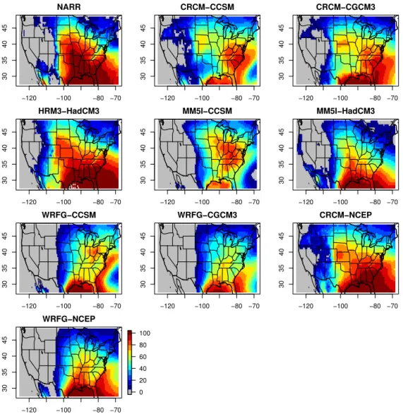
Figure 1.Images of theωfrequencies (shown as percentages per a reviewer request) for NARR and each NARCCAP model configuration.
North America. The models were run under the SRES (Na-kicenvoic and Swart, 2000) A2 scenario for the future riod 2041–2070, but also include runs for the present pe-riod 1971–2000. For verification, the models are also driven by the NCEP/Department of Energy Reanalysis II prod-uct (Kanamitsu et al., 2002) for the period 1979–2004, here-after dubbed the NCEP-driven simulations. In order to estab-lish an understanding of model uncertainty, different combi-nations of RCMs and AOGCMs are used.
Bukovsky (2012) analyzed the performance of the full set of six RCMs of the NARCCAP project driven by the NCEP reanalysis for 2 m temperature trends from 1980 to 2003. It was found that the RCMs have some capability to simulate such resolved-scale trends in the spring, and to some ex-tent, the winter. However, results for other seasons may be more dependent on the type and strength of the underlying observed forcing. Precipitation over California was consid-ered by Caldwell (2010) using all NARCCAP model outputs that provided this variable. They found that RCMs forced by
the NCEP-reanalysis tend to overpredict precipitation over California, and they concluded that this result was caused by overprediction of extreme events where otherwise the fre-quency of precipitation events was underpredicted. Interan-nual variability in NARCCAP RCMs is analyzed by de Elía et al. (2013), where it was found that important departures between RCMs and observations exist, which is also the case for some of the driving models. Nevertheless, they found that the expected climate change signal remained consistent with previous studies.
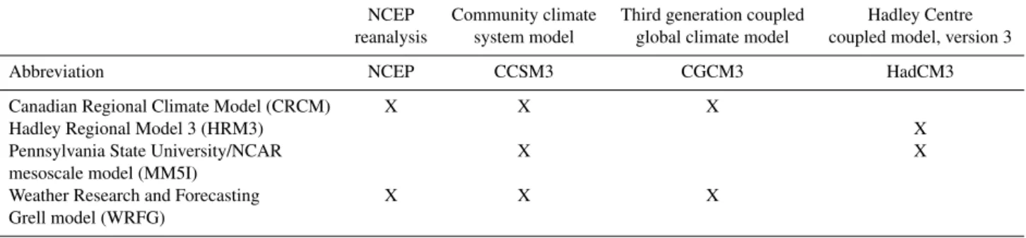
half-Table 1.Current (1971–2000) and future (2041–2070) model combinations from NARCCAP (Mearns et al., 2007,2014) analyzed in this study. NCEP-driven current-only runs.
NCEP Community climate Third generation coupled Hadley Centre reanalysis system model global climate model coupled model, version 3
Abbreviation NCEP CCSM3 CGCM3 HadCM3
Canadian Regional Climate Model (CRCM) X X X
Hadley Regional Model 3 (HRM3) X
Pennsylvania State University/NCAR X X
mesoscale model (MM5I)
Weather Research and Forecasting X X X
Grell model (WRFG)
degree grid. Because these fields are relatively smooth, the results will be relatively insensitive to the exact interpolation method used. For this work, the polynomial patch interpola-tion algorithm implemented by the Earth System Modeling Framework, which takes the local derivatives of the field in a neighborhood around the interpolation point into account, is implemented (ESMF Joint Specification Team, et al., 2014).
3 Methods
For this paper, the focus is on evaluating patterns of the large-scale indicators for severe weather conditional upon having
high field energy. Following Gilleland et al. (2013), high field energy is taken to mean that the upper quartile (over space) of the variable of interest is larger than its 90th percentile (over time). For example, from the space–time process for WmSh, a new univariate time series is calculated that represents the upper quartile of WmSh over space; this univariate time se-ries is called q75. Then, for time points when q75 is large (defined to be when it is greater than its 90th percentile over the entire time series) the frequencies of WmSh exceeding 225 m2s−2are found for each grid point, resulting in a single spatial field that summarizes where the most intense severe-storm environments are found. This resulting summary field is denotedω, and represents the frequency at each grid point when severe-storm environments occur most often. Figure 1 showsωfor the NARR and each model configuration from Table 1. Similarly, CAPE alone is also analyzed, and its conditional frequency field (for CAPE≥1000 J kg−1) is de-noted,κ (Fig. 2). For convenience, Table 2 displays some of the notations used throughout the text.
A CAPE value of 1000 J kg−1 is an arbitrary choice, but represents a value associated with severe weather environ-ments as found in previous studies (e.g., Brooks et al., 2003; Trapp et al., 2007; Gilleland et al., 2013; Heaton et al., 2011). The value of 225 m2s−2 is also an arbitrary choice, but is around the value obtained when converting CAPE from 1000 J kg−1 to Wmax and then multiplying byS=5 ms−1, which again results in a strong severe-storm environment. Of course, WmSh could have a value of 225 m2s−2 with far lower CAPE (i.e., with higher S), but because CAPE
is also conditioned to be at least 100 J kg−1 andS at least 5 m2s−2, the environment is guaranteed to be conducive to severe weather.
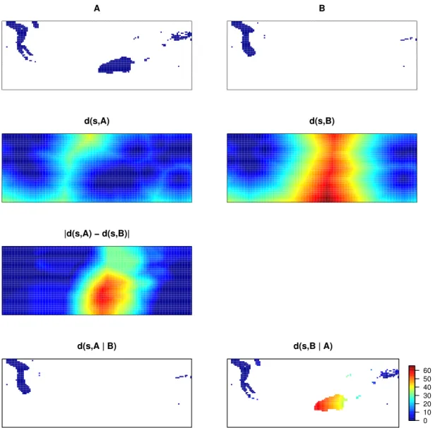
3.1 Spatial pattern and location displacement measures Several methods are available to summarize the performance of a model in terms of how well it captures the spatial pat-terns, locations, and general shape of observed variables for various thresholds of intensity, and we summarize the three used in the present study, namely: (a) Baddeley’s1, (b) mean error distance, and (c) the forecast quality index (FQI). Most of these summary measures can be calculated from distance maps (cf. Fig. 3, which shows an example). A distance map is a graphic that shows, for each grid point,x, the shortest distance from x to the nearest “event”, where an event is defined by a grid cell that exceeds the given threshold. Of particular interest is the image in the third row of the figure, which shows the absolute difference in distance maps for bi-nary fields A and B; several popular measures are derived directly from this difference field. Also of interest is to mask out the distance map A using the binary field B, and vice versa (bottom row of the figure).
The Hausdorff distance is a widely known location mea-sure that simply takes the maximum value of the absolute differences between distance maps for two fields (e.g., the maximum value from the image in the third row of Fig. 3). The metric has often been modified in order to have mea-sures that are not as sensitive to small changes in the two fields resulting from taking the maximum value. The Badde-ley1image metric (Baddeley, 1992a, b), for example, is a modification of the Hausdorff metric that replaces the maxi-mum with anLpnorm, and, in general, further modifies the
shortest distances between each grid point and the event usu-ally by setting any distances greater than a certain amount to a constant. That is,
1pf(A,B)=
1 N
X
|f(d(si,A))−f(d(si,B))|p
1/p
, (1)
func-−120 −100 −80 −70
30
35
40
45
NARR
−120 −100 −80 −70
30
35
40
45
CRCM−CCSM
−120 −100 −80 −70
30
35
40
45
CRCM−CGCM3
−120 −100 −80 −70
30
35
40
45
HRM3−HadCM3
−120 −100 −80 −70
30
35
40
45
MM5I−CCSM
−120 −100 −80 −70
30
35
40
45
MM5I−HadCM3
−120 −100 −80 −70
30
35
40
45
WRFG−CCSM
−120 −100 −80 −70
30
35
40
45
WRFG−CGCM3
−120 −100 −80 −70
30
35
40
45
CRCM−NCEP
−120 −100 −80 −70
30
35
40
45
WRFG−NCEP
0 20 40 60 80 100
Figure 2.Images of theκfrequencies for NARR and each NARCCAP model configuration.
tion on[0,∞) such thatf(x+y)≤f(x)+f(y) and is strictly increasing at zero withf(t)=0 if and only ift=0. For ex-ample, a common choice is to takef(x)=min{x,constant}. The function’s purpose is to eliminate edge effects, but the metric is highly sensitive to the choice of constant. The pa-rameterpis chosen by the user. Ifp=1 a straight average of values is achieved. The Hausdorff metric can be regained by lettingp tend to infinity. In the limit aspapproaches zero, one obtains the minimum of the portion within the absolute values of Eq. (1).
In terms of Fig. 3, Baddeley’s 1metric applies a func-tionf to each of the two fields in the second row, then takes the absolute difference between these fields, and finally takes the Lp norm over the resulting image. Following Gilleland
(2011), here,f(x)=min{x,constant}, but the constant is set to infinity andpto two, so1is simply theL2norm of the image in the third row of the figure.
The mean error distance (MED) is the mean of the dis-tance map for one field taken over only the events in the
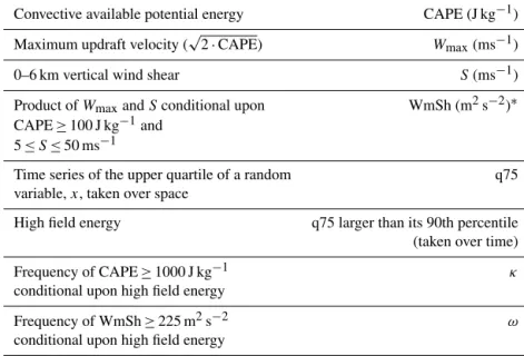
Table 2.Some notations and abbreviations used in this manuscript.
Convective available potential energy CAPE (J kg−1)
Maximum updraft velocity (√2·CAPE) Wmax(ms−1) 0–6 km vertical wind shear S(ms−1)
Product ofWmaxandSconditional upon WmSh (m2s−2)∗ CAPE≥100 J kg−1and
5≤S≤50 ms−1
Time series of the upper quartile of a random q75 variable,x, taken over space
High field energy q75 larger than its 90th percentile (taken over time)
Frequency of CAPE≥1000 J kg−1 κ
conditional upon high field energy
Frequency of WmSh≥225 m2s−2 ω
conditional upon high field energy
∗Previous studies (namely, Gilleland et al., 2013; Mannshardt and Gilleland, 2013) use the abbreviation WmSh to refer to the straight product ofWmax·S, whereas here it has the further constraint that CAPE must be at least 100 J kg−1and 5 ms−1≤S≤50 ms−1.
(average of the non-white areas in the bottom right panel) because field A has a large event that B lacks.
A further modification of the Hausdorff distance, proposed by Venugopal et al. (2005) specifically for verifying high-resolution forecasts, normalizes the measure through an av-erage of partial Hausdorff distances (PHD) obtained for sur-rogate fields, which results in a measure that, like 1, has desirable mathematical properties. It is one of the rare lo-cation metrics that also incorporates intensity information in addition to just spatial pattern information. First, stochastic realizations of the observed process that are forced to have the same Fourier spectra, probability density function, and spatial correlation structure as the observed field, called sur-rogate fields, are drawn to be used as a normalizing factor. Then, the FQI between two fields A and B, where A is the observed field, andCiis theith ofnsurrogate realizations of
A, is given by
FQI(A,B)= (2)
PHDk(A,B)
1
n
Pn
i=1PHD(A, Ci)
,
2µAµB µ2A+µ2B·
2σAσB σA2+σB2.
Here, PHDk is the partial Hausdorff distance using the kth
largest shortest distance value,µandσ denote the mean and standard deviation, respectively, over the field. The denom-inator on the right is derived from another image summary index called the universal image quality index (UIQI; Wang and Bovik, 2002), which is the denominator on the right mul-tiplied by the correlation between the two fields. Venugopal et al. (2005) refer to the denominator as the modified UIQI; the first component of which is a measure of the model field’s
bias, and the second of the variability. The UIQI ranges be-tween−1 and 1, with a value equal to one indicative of a per-fect match between the two fields. A smaller value of UIQI indicates a lot of variability.
3.2 Feature-based analysis
Numerous methods are used in meteorology that fall under the category of feature based. The idea is to identify in-dividual features within a field, and analyze those features for various characteristics, for example, those discussed in Sect. 3.1 above. In this study, the method proposed by Davis et al. (2006a) is loosely followed. In meteorological appli-cations, fields often have multiple features of interest, which would also be the case in the present context if a much larger domain were employed. However, even with a larger do-main, the relative smoothness of these climate fields results in few distinct objects. Subsequently, it is very straightfor-ward to match features between fields (e.g., as was proposed by Davis et al., 2006a, b, 2009, with the Method for Object-based Diagnostic Evaluation, or MODE), as well as to merge features within a field. The fields of κ andω demonstrate only one or two features in each model field, all of which are clearly matched with the one NARR feature that shows up. Therefore, the task is fairly simple.
be-A B
d(s,A) d(s,B)
|d(s,A) − d(s,B)|
d(s,A | B) d(s,B | A)
0 10 20 30 40 50 60
Figure 3.Top row: two binary images with dark blue showing event areas in A and B, respectively. Second row: distance maps for the images in the top row (shortest distances, in numbers of grid squares, from each pixel/grid point to an event in A or B). Third row: absolute values of the differences between the distance maps in the middle row. Bottom left: image from the second row left masked by the image from the top row right, and bottom right is the image from the second row (right) masked by the image in top row (left).
tween each field (centroid distance), the area ratio (defined to be the area of the smaller feature divided by the area of the larger one; though here the model feature areas are always smaller), the common intersection area (given as a percent), and Baddeley’s1described in section 3.1. Other properties are shown for information, but are not highly useful as com-parative measures.
3.3 Field deformation
Field deformation methods deform the spatial locations of the forecast field so that the values of the forecast variable better align with those of the observations. Numerous dif-ferent methods for deforming the field are available, and many have been proposed in the atmospheric science
In many image warping applications, the set of 0- and 1-energy control locations are easily found by hand. For ex-ample, if comparing the images of one person’s face to an-other, it is easy to choose corresponding features, such as the point of the nose or the top of the head. While it is also possible to choose the control locations by hand, an alterna-tive approach is preferred here, whereby the 1-energy con-trol locations are found through a numerical optimization procedure. The objective function to be optimized follows the approach of Aberg et al. (2005), Gilleland et al. (2010b, c), Gilleland (2013), and originally introduced by Glasbey and Mardia (2001), which is effectively the root mean square error (RMSE) between the observed and deformed forecast field plus an additional penalty term for mappings that cover too much distance or are too nonlinear. The latter term helps to prevent obtaining deformations that yield non-physical de-formations, such as folding. The penalty term includes a pre-cision matrix, or the inverse of a covariance matrix for the mappings. Aberg et al. (2005) employ a precision matrix that is zero for locations separated by a certain distance, and pos-itive otherwise, which helps to obtain deformations where nearby locations move in similar directions. In this study, the bending energy matrix, described below, is used for the de-formation, which penalizes nonlinear deformations.
The pair of thin-plate spline transformations is the bivari-ate function, 8(s)=(81(s),82(s))T =a+Gs+WTψ(s), where the set of all locations,s, in the domain isd×1 (here, the dimension d=2), and ψ(s)=(ψ(s−p0,1), . . ., ψ(s− p0,k))T, wherep0,i, i=1,2, . . ., kare the 0-energy control locations, and
ψ(h)= (3)
khkdlog(khk), if khk>0 and d mod 2=0 khkd, if khk>0 and d mod 26=0
0, else.
The mapping hasdk+d2+dparameters: (a) thed×1 vec-tor,a, (b)d×dmatrixG, and (c) thek×d matrixW, which ford=2 results in 2k+6 parameters. Thenaturalthin-plate splines used herein are subject to the further constraints that the columns of coefficients inWsum to zero (i.e.,1TW=0)
and that the sum of the products of these coefficients times the 0-energy control locations is also zero (i.e.,pT0W=0). The set of equations can be written succinctly in matrix form as
LA=
9 1k p0 1Tk 0 0 pT0 0 0
W aT GT
=
p1 0 0
. (4)
The inverse matrix, L−1, is of particular importance be-cause when performing the numerical optimization, this ma-trix needs only to be calculated one time at the beginning, and it defines the resultingwarpfunction, which is a linear function of the 1-energy control locations and the upper left
k×kpartition ofL−1, denoted byL11. That is,W=L11p1. The matrixL11is also known as thebending energy matrix
because it determines the amount of the nonlinear deforma-tion; the matricesaandGgive the linear, or affine, part of the deformation.
Note that because of the constraints onW, there are also three constraints onL11. Namely,1TkL11=0 andpT0L11=0 (recalling that p0 is k×2). The transformations imposed by Eqs. (3) and (4) minimize the total bending energy of all other possible interpolating functions from the 0-energy control locations p0 to the 1-energy control locations p1, and the total minimized bending energy (referred to hence-forth as simply the bending energy) is easily found from trace(pT1L11p
1).
In order to find theoptimalmapping ofp0 top1, the 0-energy control locations are chosen and fixed, and then the p1 locations are moved until an objective function is min-imized. Denoting the 1-energy field byZˆ and the 0-energy field byZ, the objective function used here is the same as that of Gilleland et al. (2010c), and is given by
Q(p1)= 1 2σ2
ε N
X
i=1
ˆ
Z(8(si))−Z(si)
2
+ (5)
β h
(p1−p0)TxL11(p1−p0)x+(p1−p0)TyL
11
(p1−p0)y
i ,
where thexandysubscripts denote the two component coor-dinates of the control locations,β is a penalty term chosen a priori to determine how much or little nonlinear warps should be penalized, andσεis a nuisance parameter giving the error
variance between the 0-energy and deformed 1-energy fields. The objective function (Eq. 5) results from the penalized like-lihood under an assumption of Gaussian errors between the 0-energy and deformed 1-energy fields, and potentially pro-vides a means for obtaining confidence intervals on the de-formations, but this potential will be left for future work.
3.4 Spatial prediction comparison test
The spatial prediction comparison test (SPCT) is a test intro-duced by Hering and Genton (2011) that is a spatial modi-fication of a similar time series test introduced by Diebold and Mariano (1995), and it provides a statistical hypothesis test for two competing forecast models, m1 and m2, com-pared against the same observation,athat accounts for spa-tial correlation. Hering and Genton (2011) found the test to be both powerful and of the right size provided the range of dependence is not too long, even in the face of contempora-neous correlation (i.e., whenm1is correlated withm2). First, a loss function,g, must be chosen and applied to each model against a, givingg1=g(m1, a) andg2=g(m2, a). For ex-ample, absolute error (AE) loss yieldsg(x, y)= |x−y|. Then the loss differential field,d, is calculated by taking the differ-ence at each spatial location betweeng1andg2(i.e.,g1−g2). After checking for the existence of spatial drift in the spa-tial loss differenspa-tial field, and removing any spaspa-tial trend be-fore proceeding, the empirical variogram fordis found, say
ˆ
γ, using all lags up to half of the maximum possible lag for the study region. Next, a parametric variogram model is fit toγˆ; following Hering and Genton (2011), the exponential variogram is used here. The test statistic is the usual Stu-dent’st or normal approximation for the paired sample test of the mean of the loss differential field, but where the stan-dard error is estimated by averaging the values from the spa-tial correlation function, by way of a linear combination of the parametric variogram fit toγˆover all lags of the domain. In other words, the test statistic,Sv, to test whether or not the
mean loss differential,d, is significantly different from zero is
Sv=
d b
se(d), (6)
where
b
se(d)=sX
i
X
j
[ ˆγ(∞; ˆθ)− ˆγ(hij; ˆθ)], (7)
with θˆ estimated parameters of the parametric variogram model evaluated at each lag hij. Because the spatial fields
presently studied all have a reasonably large number of grid points, the normal approximation of the test is used through-out.
Here, the test is conducted under AE loss first, and then with AE+deformation loss for comparison. The latter was proposed by Gilleland (2013), and allows for both spatial displacement/pattern error and intensity errors to be simulta-neously incorporated into the test, while also accounting for spatial correlation. The loss is achieved by finding the AE be-tween the observed field and the deformed forecast field (cf. Sect. 3.3) and adding these errors to the (Euclidean) distance each point “traveled” in order to achieve the re-aligned field.
0 20 40 60 80
0 5 10 15 Threshold (percentile) B a d d e le y 's de lt a m e tr ic ● ● ● ● ● ● ● ● ● ● ● ● ● ● ● ● ● ● ● ● ● ● ● ● ● ● ●
0 20 40 60 80
0
5
10
15
Threshold (percentile)
Mean error distance (F
, O) ● ● ● ● ● ● ● ● ● ● ● ● ● ● ● ● ● ● ● ● ● ● ● ● ● ● ●
0 20 40 60 80
0
5
10
15
Threshold (percentile)
Mean error distance (O
, F) ● ● ● ● ● ● ● ● ● ● ● ● ● ● ●● ● ● ● ● ● ● ● ●● ● ●
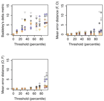
Figure 4.Baddeley’s1(p=2,c= ∞; top left), mean error dis-tance conditioning on observed events (top right) and mean er-ror distance conditioning on “forecast” events (bottom left) forκ. Shapes indicate the regional model: CRCM (circles), HRM3 (dia-monds), MM5I (squares), and WRFG (triangles). Colors indicate the driving models: CCSM3 (black), CGCM3 (gray), HadCM3 (blue), NCEP (orange).
4 Results
Figure 4 shows the results for the location measures forω, the frequency of WmSh greater than 225 m2s−2conditional on high field energy (see Table 2 for notation). It can be ar-gued from visual inspection of the graphic that the models driven by the HadCM3 global model are closest to reproduc-ing the patterns ofωassociated with the NARR reanalysis. This result is consistent across the thresholds for mean error distance, but the HRM3–HadCM3 has higher (worse) Bad-deley1metric values for the highest thresholds. In terms of capturing the spatial structure of the most frequent events for WmSh, the CCSM3-driven runs are the least similar to those found in the NARR, and the WRFG–CGCM3 performs the worst in terms of capturing the spatial patterns ofωaccording to the Baddeley1metric; the results forκ (not shown) are similar. Of course, these results do not account for sampling uncertainty, so no conclusions can be made with statistical significance based on these measures.
A feature-based analysis is also conducted (Tables 3 and 4), which provides similar, but more detailed information about how the fields compare to one another. Tables 3 and 4 show summary statistics for identifiedωfeatures (Table 3) and feature comparisons for matched (possibly first merged) ωfeatures (Table 4) after having set a threshold of having at least 75 % frequency of occurrence.1In each case, it is clear
1The values in the table are calculated using the R(R Core Team,
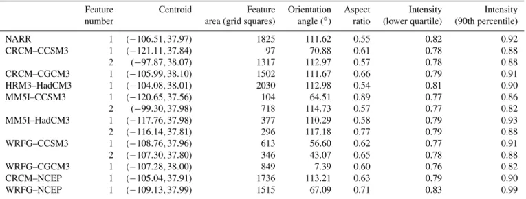
Table 3.Feature identification and properties for frequency ofω. Features identified using a threshold of 75 % frequency.
Feature Centroid Feature Orientation Aspect Intensity Intensity number area (grid squares) angle (◦) ratio (lower quartile) (90th percentile)
NARR 1 (−106.51,37.97) 1825 111.62 0.55 0.82 0.92
CRCM–CCSM3 1 (−121.11,37.84) 97 70.88 0.61 0.78 0.88
2 (−97.87,38.07) 1317 112.97 0.57 0.78 0.88 CRCM–CGCM3 1 (−105.99,38.10) 1502 111.67 0.66 0.79 0.91 HRM3–HadCM3 1 (−104.08,38.01) 2030 112.98 0.54 0.81 0.90
MM5I–CCSM3 1 (−120.65,37.56) 104 64.51 0.89 0.77 0.86
2 (−99.30,37.98) 718 114.73 0.57 0.77 0.82
MM5I–HadCM3 1 (−117.76,37.98) 377 110.29 0.58 0.79 0.93 2 (−116.14,37.81) 296 117.18 0.77 0.79 0.88
WRFG–CCSM3 1 (−108.76,37.96) 613 56.60 0.62 0.77 0.91
2 (−107.30,37.80) 346 43.07 0.65 0.78 0.88
WRFG–CGCM3 1 (−107.28,38.00) 849 7.39 0.60 0.76 0.82
CRCM–NCEP 1 (−105.04,37.91) 1736 113.21 0.63 0.79 0.90
WRFG–NCEP 1 (−109.13,37.99) 1515 67.09 0.71 0.83 0.99
Table 4. Merged and matched feature comparisons forω. Features identified using a threshold of 75 % frequency. Minimum boundary separation is zero for all comparisons. Total interest is given in parentheses below model name.
Features compared Centroid distance Angle Area Intersection Bearing Baddeley1
(NARR vs. model) (grid squares) difference (◦) ratio area (◦from north) (p=2,c= ∞)
CRCM–CCSM3 1 vs. (1 and 2) 7.05 46.99 0.77 0.69 88.74 2.98
CRCM–CGCM3 1 vs. 1 0.53 0.05 0.82 0.85 107.77 2.39
HRM3–HadCM3 1 vs. 1 2.42 1.36 0.90 0.90 90.42 3.43
MM5I–CCSM3 1 vs. (1 and 2) 4.50 4.37 0.45 0.59 87.99 7.82
MM5I–HadCM3 1 vs. (1 and 2) 10.54 33.58 0.37 0.54 −86.34 13.128
WRFG–CCSM3 1 vs. (1 and 2) 1.73 44.21 0.53 0.63 −86.73 10.74
WRFG–CGCM3 1 vs. 1 0.77 44.23 0.47 0.62 −93.00 12.14
CRCM–NCEP 1 vs. 1 1.47 1.60 0.95 0.91 86.80 1.52
WRFG–NCEP 1 vs. 1 2.62 44.52 0.83 0.90 −89.77 7.88
that the HRM3–HadCM3 does the best job of all of the mod-els at achieving a roughly correct spatial pattern for the most frequentωareas. It has a relatively low centroid distance, an-gle difference, and Baddeley1value, as well as one of the highest area ratios (0.90) and intersection areas (also 0.90; tied for highest with WRFG–NCEP). Moreover, it has the same number of identified features above the 75 % threshold as the NARR. For all of the fields, the largest feature is in the southeast corner of the domain over the ocean, and in most cases hugs the border, suggesting that high CAPE would be modeled beyond the edge of the domain. Results forκ (not shown) are similar. The bearing is calculated from the model feature centroid to the NARR feature centroid with north as the reference, which simply gives a sense of the direction in which the features of one field are situated with respect to the other. For a model whose output variable has small sepa-ration distance and good area overlap with the observed
fea-the package spatstat (Baddeley and Turner, 2005). Orientation angle and aspect ratio are found with help from package smatr (Warton et al., 2012).
ture (e.g., CRCM–CGCM3), the bearing is perhaps not very meaningful. However, for those with larger separation dis-tances and less area overlap (e.g., the models here have fairly good spatial pattern matches, but MM5I–HadCM3 is a can-didate for checking the bearing to see if the problem exists for other variables), then the bearing could prove useful to a modeler hoping to diagnose how the model failed.
At lower thresholds than 75 % frequency (not shown), an additional area of high frequency is generally observed in the southwest near or over Baja California. Careful inspection of models using the CCSM3 as the driving model reveals that there is a tendency for more numerous, but smaller, features than produced by the NARR or other driving models (cf. Ta-ble 3). In each case, these disjoint features are merged (using centroid distance as the primary criterion) before comparing with the NARR as they are primarily located in the southeast region.
Table 5. Results from deforming climate models to better spa-tially align with NARR reanalysis for κ. RMSE0 is the original RMSE, RMSE1the resulting RMSE between the deformed model and NARR, and the bending energy is a summary measure of the amount of nonlinear deformations applied to deform the field.
RMSE0 RMSE1 % RMSE Bending reduction energy
CRCM–CCSM3 0.214 0.1393 35 0.9555 CRCM–CGCM3 0.1467 0.1028 30 1.0739 HRM3–HadCM3 0.1569 0.11 30 0.2531 MM5I–CCSM3 0.2665 0.1605 40 2.0042 MM5I–HadCM3 0.1477 0.084 43 0.6933 WRFG–CCSM3 0.2493 0.0961 61 3.2692 WRFG–CGCM3 0.2406 0.0918 62 3.3178 CRCM–NCEP 0.214 0.1727 19 0.2545 WRFG–NCEP 0.1711 0.0923 46 0.4304
called total interest that incorporates user-specified weights in order to obtain a measure based on the attributes of a fea-ture that are most important. It ranges between zero and 1 where a value of 1 indicates a perfect match and the worst value is zero. The technique is performed for these fea-tures using the same interest maps and weights as proposed in Davis et al. (2006a). All of the total interest values are very high, ranging from 0.91 to 0.94, indicating good agreement between the models and the NARR.
It is also of interest to determine if one model stands out above others. To do so, we use the SPCT with AE loss, which is a very conservative test because small-scale errors and spatial displacements are not taken into account, and none of the results is statistically significant at any reason-able level suggesting that the null hypothesis of equal perfor-mance (as measured by the mean AE loss differential) can-not be rejected. In order to factor in spatial alignment and small-scale errors to the test, the SPCT is also applied with AE+deformation loss following Gilleland (2013).
Indeed, inspection of the graphs of κ (Fig. 2) clearly re-veals that some models capture the spatial patterns of the high-event frequency CAPE areas better than others. Field deformation techniques are well-established methods for verifying forecasts spatially where small mis-alignments in space obfuscate model performance. Table 5 displays the re-sults of having found the optimal deformation for each model deformed to better align spatially with the NARR reanalysis. Shown are the original RMSE, denoted RMSE0, the RMSE after having applied the optimal deformation, RMSE1, the percent reduction in RMSE, and the minimum bending en-ergy required to arrive at the optimal re-alignment. The mini-mum bending energy is not a summary of the entire deforma-tion, only the non-affine ones. Thus, a small bending energy does not imply that the deformation is necessarily small, but rather that nonlinear distortions are not abundant. However, the bending energy is useful as a comparison because a field,
A, with higher bending energy than a field, B, implies that A matches less well than B with the 0-energy field in terms of overall shapes of patterns. A perfect model would have zero RMSE0and thus no reduction in error or bending energy. A good model will have a low RMSE0paired with low bend-ing energy and often a relatively high reduction in error. A bad model will have relatively high RMSE0and either high reduction in error paired with high bending energy, or low reduction in error paired with low bending energy.
Figures 5–7 display examples of the resulting field de-formations for κ, for typical deformations for these cases (Fig. 5), the HRM3–HadCM3 (Fig. 6), which requires very little deformation because the original field is already closely aligned with the NARR, and a case where the spatial align-ment (and intensities) are fairly poor; resulting in a more tor-tured deformation (Fig. 7). In most cases, a small amount of affine and nonlinear deformation results in considerable error reduction. The cases that require more nonlinear de-formations (MM5I–CCSM3, WRFG–CCSM3, and WRFG– CGCM3; latter two not shown) stand out in both the “dis-tance traveled” and “deformed 1-energy” panels for requiring a relatively large amount of deformation in order to match well with the NARR data product.
Severe thunderstorms require high CAPE, which is basi-cally a measure of the amount of energy available to cre-ate very strong updrafts in thunderstorms. High CAPE en-vironments have a warm, moist boundary layer, with colder air aloft, the latter of which increases conditional instability. Proximity to warm, large bodies of water in the domain (i.e., the Gulf of Mexico, Caribbean, and Gulf of California) plays a large role in dictating the spatial distribution of high CAPE in the domain as they are the primary sources of moisture. Moisture transport mechanisms also play a role. High CAPE does not often occur at high elevation or near the west coast because near-surface moisture is too low and/or near-surface temperature is too cold. In the CCSM3-driven simulations, the RCMs inherit an atmosphere that is too dry from the CCSM3 in the warm season (Bukovsky and Karoly, 2010; Bukovsky et al., 2013). This dryness would strongly effect the frequency of high CAPE values in the central part of the country during the dominant season for severe weather in the region. In the MM5I vs. the CRCM–CCSM3-driven simula-tions, it is likely that moisture transport mechanisms simu-lated by the regional models are playing a strong role in dic-tating the distribution of moisture, thus resulting in the spa-tial distribution of high CAPE frequencies east of the Missis-sippi River. In the HRM3–HadCM3, it is likely that warm-season low level winds are a bit too southeasterly through the Plains, carrying more moisture into the High Plains and Rocky mountain region than is observed, leading to the high CAPE frequencies seen from central Mexico north through Wyoming and eastern Montana.
er-Figure 5.Deformation results forκ. Top left is NARR reanalysis (0-energy field), top middle is CRCM–CCSM3 (1-energy field), top right is the error between NARR and CRCM–CCSM3. Bottom left shows the distance that the intensity “traveled” to arrive at each grid point, bottom middle is the deformed CRCM–CCSM3 field, and bottom right is the error field between NARR and the deformed CRCM–CCSM3.
Figure 6.Same as Fig. 5, but for HRM3–HadCM3.
ror. Indeed, the WRFG model combinations had some of the worst spatial alignment with the NARR, so the im-provement induced by re-alignment is the most drastic. It should be noted, however, that the deformations for the two WRFG cases, WRFG–CCSM3 and WRFG–CGCM3, also have the largest amount of nonlinear deformation with min-imum bending energies much greater than any other model combinations. Inspection of the graphs of the deformations (not shown) suggests that the linear deformations are also large for these cases. HRM3–HadCM3 has the least amount of bending energy, and only a small amount of affine dis-placements from the NARR. Nevertheless, with only a small
amount of deformation, this model still achieves a reduction in RMSE, which is small to begin with, by almost 30 %.
Figure 7.Same as Fig. 5, but for MM5I–CCSM3.
Table 6.Same as Table 5, but forω.
RMSE0 RMSE1 % RMSE Bending reduction energy
CRCM–CCSM3 0.1313 0.1006 23 0.0228 CRCM–CGCM3 0.1081 0.0966 11 1.1484 HRM3–HadCM3 0.0977 0.0673 31 0.265 MM5I–CCSM3 0.1802 0.1101 39 5.988 MM5I–HadCM3 0.1308 0.091 30 1.132 WRFG–CCSM3 0.1849 0.0914 51 0.9347 WRFG–CGCM3 0.1948 0.1087 44 0.8507 CRCM–NCEP 0.0939 0.0781 17 0.2466 WRFG–NCEP 0.1242 0.0704 43 0.5423
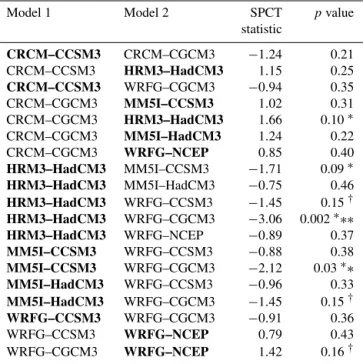
Following Gilleland (2013), the SPCT is applied with AE plus deformation loss induced by the above deformations. Some relatively significant results are now found; including one case with better than 1 % significance, one with better than 5 % significance, two cases with better than 10 % sig-nificance, and three with about 15 % significance. Table 7 displays the test results for the cases where thepvalue is less than 0.50. As mentioned above, the HRM3–HadCM3 model appears to be the closest to the NARR in terms of spatial pat-tern and location, as well as having about the right frequen-cies in these areas; only a relatively small amount of defor-mation is needed to optimize the alignment. Subsequently, it is no surprise that this model is shown to be better than all the other models; three of which are significantly bet-ter at the 10 % level or betbet-ter according to the SPCT with AE+deformation loss. Models with the HadCM3 compo-nent generally fared very well under this test, and the MM5I combinations also fared well. In general, the worse models failed to capture the spatial extent of areas with frequently
Table 7.SPCT results when AE+deformation loss is applied to
κ. Results shown are only for those cases with pvalues≤50%. Values shown are the mean loss differential statistic and associated
pvalue in parentheses. Bold face emphasizes the “better” model according to the test; where negative (positive) values mean model 1 (model 2) is better. (∗∗∗) indicates significance at the≈0 % level, (∗∗) at the 5 % level, (∗) at the 10 % level, (†) at the 20 % level. Note, the CRCM–NCEP case is not included because a good-fitting variogram could not be found for any of the loss differential fields associated with this model.
Model 1 Model 2 SPCT pvalue
statistic
CRCM–CCSM3 CRCM–CGCM3 −1.24 0.21 CRCM–CCSM3 HRM3–HadCM3 1.15 0.25
CRCM–CCSM3 WRFG–CGCM3 −0.94 0.35 CRCM–CGCM3 MM5I–CCSM3 1.02 0.31 CRCM–CGCM3 HRM3–HadCM3 1.66 0.10∗ CRCM–CGCM3 MM5I–HadCM3 1.24 0.22 CRCM–CGCM3 WRFG–NCEP 0.85 0.40
HRM3–HadCM3 MM5I–CCSM3 −1.71 0.09∗
HRM3–HadCM3 MM5I–HadCM3 −0.75 0.46
HRM3–HadCM3 WRFG–CCSM3 −1.45 0.15†
HRM3–HadCM3 WRFG–CGCM3 −3.06 0.002∗∗∗
HRM3–HadCM3 WRFG–NCEP −0.89 0.37
MM5I–CCSM3 WRFG–CCSM3 −0.88 0.38
MM5I–CCSM3 WRFG–CGCM3 −2.12 0.03∗∗
MM5I–HadCM3 WRFG–CCSM3 −0.96 0.33
MM5I–HadCM3 WRFG–CGCM3 −1.45 0.15†
Table 8.Same as Fig. 7, but forω.
Model 1 Model 2 SPCT pvalue
statistic
CRCM–CCSM3 CRCM–CGCM3 −1.09 0.27
CRCM–CCSM3 MM5I–CCSM3 −1.31 0.19∗
CRCM–CCSM3 MM5I–HadCM3 −0.84 0.40
CRCM–CCSM3 WRFG–CCSM3 −1.03 0.30
CRCM–CCSM3 WRFG–CGCM3 −0.82 0.41
CRCM–CGCM3 CRCM–NCEP 0.76 0.45
HRM3–HadCM3 MM5I–CCSM3 −1.64 0.10∗
HRM3–HadCM3 MM5I–HadCM3 −0.82 0.41 HRM3–HadCM3 WRFG–CCSM3 −1.26 0.21 HRM3–HadCM3 WRFG–CGCM3 −0.8 0.43 MM5I–CCSM3 WRFG–CCSM3 0.9 0.37 MM5I–CCSM3 WRFG–CGCM3 0.85 0.40 MM5I–CCSM3 CRCM–NCEP 1.63 0.10∗
MM5I–CCSM3 WRFG–NCEP 1.38 0.17∗
MM5I–HadCM3 CRCM–NCEP 0.82 0.41 WRFG–CCSM3 CRCM–NCEP 1.76 0.08∗ WRFG–CCSM3 WRFG–NCEP 1.36 0.17∗ WRFG–CGCM3 CRCM–NCEP 1.33 0.18∗ WRFG–CGCM3 WRFG–NCEP 1.36 0.17∗
CRCM–NCEP WRFG–NCEP −0.76 0.45
high values of CAPE and WmSh. They tend to miss, or un-derpredict, the high-frequencies in the northwest extending to eastern Colorado and Wyoming compared with NARR. They also tend to project considerably less frequency in the southwestern part of the domain.
Despite the fact that theωdeformation results are similar to those forκ, the SPCT with AE+deformation loss results are less similar. However, the HRM3 configurations do still tend to outperform other models, in one case with statistical significance at almost the 10 % level (Table 8).
5 Conclusions
In this study, several advanced weather forecast verification techniques for high-resolution gridded verification sets are applied in a novel way to severe-storm indicators from sev-eral of the North American Climate Change Assessment Pro-gram (NARCCAP) climate models. In particular, focus is placed on the distributional property of how well the models capture the frequencies of severe-storm environments when the field energy is high, where field energy is defined by the upper quartile over space and this field energy is considered to be high when it is in the upper 90th percentile over time. For ease of discussion, we denoteκ to be the frequency of CAPEs exceeding 1000 J kg−1 conditional upon high field energy for CAPE, and similarly, ω to be the frequency of WmSh’s exceeding 225 m2s−2 conditional upon high field energy for WmSh, where WmSh is equal to√2·CAPE·S, andSdenotes 0–6 km vertical wind shear (ms−1), provided
that CAPE≥100 J kg−1 and 5≤S≤50 (zero otherwise). Previous studies found concurrently high values of CAPE andSto be important indicators of severe-storm activity, and the derived WmSh indicator from these coarse-scale vari-ables discriminates severe-storm activity well as a univariate variable.
In general, the NARCCAP runs under estimate the spatial extent of high frequencyκandωwhere the HRM3–HadCM3 model run performs the best; having an area ratio near unity at≈90 % and an intersection area of about 89 % forκ and about 90 % in both categories forω. The CRCM–NCEP run is the next best in this regard with only slightly lower ratios. Forω the numbers are similar for these models, although the CRCM–NCEP has slightly better overlap (intersection area about 0.91 vs. 0.84) and the CRCM–CGCM3 also has a high area ratio (0.82 vs. 0.60) and intersection area (0.85 vs. 0.66). Otherwise, the area ratios for high frequencies for most models range between about 20 and 60 % (0.91 for HRM3– HadCM3) forκand between about 35 and 95 % forω; results are similar for intersection area for both frequencies.
The application of binary image metrics suggests that overall the models do reasonably well at capturing high-frequencies ofκ andω, but for the very high-frequency ar-eas, some models perform less well. In particular, mean error distance and Baddeley’s 1 are applied, and for thresholds above 80 %, it is found that the best models at capturingκ are those that drive the regional models HRM3 and WRFG. The worst at capturing the spatial patterns forκ are those with CRCM and MM5I regional models, as well as those driven by CCSM3 and CGCM3. Forω, the runs with NCEP as the driving model perform worse at capturing frequency area patterns for frequencies above about 80%, as well as those utilizing CCSM3 and CGCM3.
also performs well. The MM5I regional model is generally outperformed by other models.
The utility of applying spatial forecast verification tech-niques for climate model evaluation studies is presented, and the results of this study for severe-storm environments pro-vide important insight into how to interpret future model runs for these NARCCAP models. In particular, caution is re-quired when considering very high frequencies forω, and fo-cus should be restricted to more moderate thresholds. More-over, the spatial extent of future storm environments may be an underestimation from nearly all of the model runs, and more weight should be put on the HRM3–HadCM3 run than other models, with considerably less weighting on model combinations involving CGCM3.
Some methods provide analogous information, which pro-vides consistency in ascertaining model performance, but each can provide its own unique perspective depending on the fields in question. For example, image warping is a highly complicated approach, which could be considered unneces-sary for simply inferring about how far off each model is from the NARR. On the other hand, it provides the only method known to the current authors that provides a statisti-cal hypothesis test (or confidence intervals) that accounts for both spatial correlation and displacement errors. The binary image metrics such as the Hausdorff, partial Hausdorff, and Baddeley1all provide distributional summaries of the abso-lute difference in distance maps between two binary “event” fields, with1providing arguably the most useful informa-tion. A summary of these measures can be found in Badde-ley (1992a, b) and Schwedler and Baldwin (2011). The FQI incorporates such displacement information, but also inten-sity information so that it may provide redundant information as these other distance map-based measures, but depending on the intensities, it could also yield different results. The feature-based approaches utilize many of these same types of information, but inform about specific features within a field, which in the present case is less important, but does de-scribe how some models have two smaller features instead of one large feature (i.e., area of higher frequencyκ/ω).
6 Data availability
For NARR, the data can be accessed from EMC (http://www. emc.ncep.noaa.gov/mmb/rreanl/) (EMC, 2007). The North American Regional Climate Change Assessment Program data set is available at doi:10.5065/D6RN35ST (Mearns et al., 2007, 2014).
Acknowledgements. Support for this manuscript was provided by the Weather and Climate Impact Assessment Science Program (http://www.assessment.ucar.edu) at the National Center for Atmospheric Research (NCAR) with additional support from the National Science Foundation (NSF) through Earth System Model-ing (EaSM) grant number AGS-1243030. NCAR is sponsored by
NSF and managed by the University Corporation for Atmospheric Research. We wish to thank the North American Regional Climate Change Assessment Program (NARCCAP) for providing the data used in this paper. NARCCAP is funded by the National Science Foundation (NSF), the US Department of Energy (DoE), the National Oceanic and Atmospheric Administration (NOAA), and the US Environmental Protection Agency Office of Research and Development (EPA). Software used in this article is from the R (R Core Team, 2015) packageSpatialVx (Gilleland, 2016a), which draws largely on functions from thespatstatpackage (Baddeley and Turner, 2005; Baddeley et al., 2015).
Edited by: S.-K. Min
Reviewed by: two anonymous referees
References
Aberg, S., Lindgren, F., Malmberg, A., Holst, J., and Holst, U.: An image warping approach to spatio-temporal modelling, Environ-metrics, 16, 833–848, 2005.
AghaKouchak, A. and Mehran, A.: Extended contingency table: Performance metrics for satellite observations and climate model simulations, Water Resour. Res., 49, 7144–7149, 2013. AghaKouchak, A., Nasrollahi, N., Li, J., Imam, B., and Sorooshian,
S.: Geometrical Characterization of Precipitation Patterns, J. Hy-drometeorol., 12, 274–285, 2010.
Ahijevych, D., Gilleland, E., Brown, B. G., and Ebert, E. E.: Appli-cation of Spatial VerifiAppli-cation Methods to Idealized and NWP-Gridded Precipitation Forecasts, Weather Forecast., 24, 1485– 1497, 2009.
Alemohammad, S. H., McLaughlin, D. B., and Entekhabi, D.: Quantifying Precipitation Uncertainty for Land Data Assimila-tion ApplicaAssimila-tions, Mon. Weather Rev., 143, 3276–3299, 2015. Alexander, G. D., Weinman, J. A., and Schols, J. L.: The Use of
Digital Warping of Microwave Integrated Water Vapor Imagery to Improve Forecasts of Marine Extratropical Cyclones, Mon. Weather Rev., 126, 1469–1496, 1998.
Arbogast, P., Pannekoucke, O., Raynaud, L., Lalanne, R., and Mémin, E.: Object-oriented processing of CRM precipitation forecasts by stochastic filtering, Q. J. Roy. Meteor. Soc., qJ-15-0353.R2, doi:10.1002/qj.2871, 2016.
Baddeley, A. J.: Errors in binary images and an Lp version of the Hausdorff metric, Nieuw Arch. Wiskunde, 10, 157–183, 1992a. Baddeley, A. J.: Robust Computer Vision Algorithms, chap. An
er-ror metric for binary images, 59–78, edited by: Forstner, W. and Ruwiedel, S., Wichmann, 402 pp., 1992b.
Baddeley, A. J. and Turner, R.: spatstat: An R package for analyzing spatial point patterns, J. Stat. Softw., 12, 1–42, 2005.
Baddeley, A. J., Rubak, E., and Turner, R.: Spatial Point Patterns: Methodology and Applications with R, Chapman and Hall/CRC Reference, 810 pp., 408 B/W Illustrations, ISBN-13: 9781482210200, CAT# K21641, available at: https://www.crcpress.com/ Spatial-Point-Patterns-Methodology-and-Applications-with-R/ Baddeley-Rubak-Turner/p/book/9781482210200, 2015. Brooks, H. E., Lee, J. W., and Craven, J. P.: The spatial distribution
Brown, B. G., Gilleland, E., and Ebert, E. E.: Forecasts of Spa-tial Fields, chap. 6, 95–117, in: Forecast Verification: A Prac-titioner’s Guide in Atmospheric Science, edited by: Jolliffe, I. T. and Stephenson, D. B., John Wiley & Sons, Ltd, 274 pp., 2011. Bukovsky, M. S.: Temperature trends in the NARCCAP Regional
Climate Models, J. Climate, 25, 3985–3991, 2012.
Bukovsky, M. S. and Karoly, D. J.: A Regional Modeling Study of Climate Change Impacts on Warm-Season Precipitation in the Central United States, J. Climate, 24, 1985–2002, 2010. Bukovsky, M. S., Gochis, D. J., and Mearns, L. O.: Towards
As-sessing NARCCAP Regional Climate Model Credibility for the North American Monsoon: Current Climate Simulations, J. Cli-mate, 26, 8802–8826, 2013.
Caldwell, P.: California wintertime precipitation bias in Regional and Global Climate Models, J. Appl. Meteorol. Clim., 49, 2147– 2158, 2010.
Carley, J. R., Schwedler, B. R. J., Baldwin, M. E., and Trapp, R. J.: A proposed model-based methodology for feature-specific pre-diction for high-impact weather, Weather Forecast., 26, 243–249, 2011.
Davis, C., Brown, B., and Bullock, R.: Object-Based Verification of Precipitation Forecasts. Part I: Methodology and Application to Mesoscale Rain Areas, Mon. Weather Rev., 134, 1772–1784, 2006a.
Davis, C., Brown, B., and Bullock, R.: Object-Based Verification of Precipitation Forecasts. Part II: Application to Convective Rain Systems, Mon. Weather Rev., 134, 1785–1795, 2006b.
Davis, C. A., Brown, B. G., Bullock, R., and Halley-Gotway, J.: The Method for Object-Based Diagnostic Evaluation (MODE) Ap-plied to Numerical Forecasts from the 2005 NSSL/SPC Spring Program, Weather Forecast., 24, 1252–1267, 2009.
de Elía, R., Biner, S., and Frigon, A.: Interannual variability and ex-pected regional climate change over North America, Clim. Dy-nam., 41, 1245, doi:10.1007/s00382-013-1717-9, 2013. Diebold, F. X. and Mariano, R. S.: Comparing Predictive Accuracy,
J. Bus. Econ. Stat., 13, 253–263, 1995.
Diffenbaugh, N. S., Scherer, M., and Trapp, R. J.: Robust in-creases in severe thunderstorm environments in response to greenhouse forcing, P. Natl. Acad. Sci. USA, 110, 16361–16366, doi:10.1073/pnas.1307758110, 2013.
Dryden, I. L. and Mardia, K. V.: Statistical shape analysis, John Wiley & Sons, Chichester, ISBN-10: 0470699620, 1998. Elsner, J. B., Elsner, S. C., and Jagger, T. H.: The increasing
effi-ciency of tornado days in the United States, Clim. Dynam., 45, 651–659, 2015.
EMC: National Centers for Environmental Prediction (NCEP), North American Regional Reanalysis (NARR), available at: http: //www.emc.ncep.noaa.gov/mmb/rreanl/, 2007.
ESMF Joint Specification Team: Balaji, V., Boville, B., Collins, N., Craig, T., Cruz, C., da Silva, A., DeLuca, C., Eaton, B., Hallberg, B., Hill, C., Iredell, M., Jacob, R., Jones, P., Kauffman, B., Lar-son, J., Michalakes, J., Neckels, D., Panaccione, C., Rosinski, J., Schwab, E., Smithline, S., Suarez, M., Swift, S., Theurich, G., Vasquez, S., Wolfe, J., Yang, W., Young, M., and Zaslavsky, L.: ESMF Reference Manual for Fortran, version 6.3.Orp1, 2014. Gensini, V. A., Ramseyer, C., and Mote, T. L.: Future convective
environments using NARCCAP, Int. J. Climatol., 34, 1699–1705, 2014.
Gilleland, E.: Spatial Forecast Verification: Baddeley’s Delta Metric Applied to the ICP Test Cases, Weather Forecast., 26, 409–415, 2011.
Gilleland, E.: Testing Competing Precipitation Forecasts Accu-rately and Efficiently: The Spatial Prediction Comparison Test, Mon. Weather Rev., 141, 340–355, 2013.
Gilleland, E.: SpatialVx: Spatial Forecast Verification, National Center for Atmospheric Research, Boulder, Colorado, USA, R package version 0.5, 2016a.
Gilleland, E.: A new characterization in the spatial verification framework for false alarms, misses, and overall patterns, Weather Forecast., available at: http://journals.ametsoc.org/page/eors, ac-cepted, 2016b.
Gilleland, E., Ahijevych, D., Brown, B. G., Casati, B., and Ebert, E. E.: Intercomparison of Spatial Forecast Verification Methods, Weather Forecast., 24, 1416–1430, 2009.
Gilleland, E., Ahijevych, D. A., Brown, B. G., and Ebert, E. E.: Verifying Forecasts Spatially, B. Am. Meteorol. Soc., 91, 1365– 1373, 2010a.
Gilleland, E., Chen, L., DePersio, M., Do, G., Eilertson, K., Jin, Y., Lang, E., Lindgren, F., Lindström, J., Smith, R., and Xia, C.: Spa-tial forecast verification: image warping, Tech. Rep. NCAR/TN-482+STR, NCAR, 2010b.
Gilleland, E., Lindström, J., and Lindgren, F.: Analyzing the image warp forecast verification method on precipitation fields from the ICP, Weather Forecast., 25, 1249–1262, 2010c.
Gilleland, E., Brown, B., and Ammann, C.: Spatial extreme value analysis to project extremes of large-scale indicators for severe weather, Environmetrics, 24, 418–432, 2013.
Glasbey, C. A. and Mardia, K. V.: A penalized likelihood approach to image warping, J. R. Statist. Soc. B, 63, 465–514, 2001. Heaton, M. J., Katzfuss, M., Ramachandar, S., Pedings, K.,
Gille-land, E., Mannshardt-Shamseldin, E., and Smith, R. L.: Spatio-temporal models for large-scale indicators of extreme weather, Environmetrics, 22, 294–303, 2011.
Hering, A. S. and Genton, M. G.: Comparing Spatial Predictions, Technometrics, 53, 414–425, 2011.
Hoffman, R. N. and Grassotti, C.: A Technique for Assimilating SSM/I Observations of Marine Atmospheric Storms: Tests with ECMWF Analyses, J. Appl. Meteorol., 35, 1177–1188, 1996. Hoffman, R. N., Liu, Z., Louis, J.-F., and Grassoti, C.:
Distor-tion RepresentaDistor-tion of Forecast Errors, Mon. Weather Rev., 123, 2758–2770, 1995.
Kanamitsu, M., Ebisuzaki, W., Woollen, J., Yang, S.-K., Hnilo, J. J., Fiorino, M., and Potter, G. L.: NCEP–DOE AMIP-II Reanalysis (R-2), B. Am. Meteorol. Soc., 83, 1631–1643, 2002.
Keil, C. and Craig, G. C.: A Displacement-Based Error Mea-sure Applied in a Regional Ensemble Forecasting System, Mon. Weather Rev., 135, 3248–3259, 2007.
Keil, C. and Craig, G. C.: A Displacement and Amplitude Score Employing an Optical Flow Technique, Weather Forecast., 24, 1297–1308, 2009.
Kleiber, W., Sain, S., and Wiltberger, M.: Model Calibration via Deformation, SIAM/ASA Journal on Uncertainty Quantification, 2, 545–563, 2014.
per-ception and evaluated against a modeling case study, Water Re-sour. Res., 51, 1225–1246, 2015.
Koch, J., Siemann, A., Stisen, S., and Sheffield, J.: Spatial val-idation of large-scale land surface models against monthly land surface temperature patterns using innovative perfor-mance metrics, J. Geophys. Res.-Atmos., 121, 5430–5452, doi:10.1002/2015JD024482, 2016.
Levy, A. A. L., Ingram, W., Jenkinson, M., Huntingford, C., Hugo Lambert, F., and Allen, M.: Can correcting feature loca-tion in simulated mean climate improve agreement on projected changes?, Geophys. Res. Lett., 40, 354–358, 2013.
Li, J., Hsu, K., AghaKouchak, A., and Sorooshian, S.: An object-based approach for verification of precipitation estimation, Int. J. Remote Sens., 36, 513–529, 2015.
Li, J., Hsu, K.-L., AghaKouchak, A., and Sorooshian, S.: Object-based assessment of satellite precipitation products, Remote Sens., 8, 547, doi:10.3390/rs8070547, 2016.
Mannshardt, E. and Gilleland, E.: Extremes of Severe Storm En-vironments under a Changing Climate, American J. Climate Change, 2, 47–61, 2013.
Marzban, C. and Sandgathe, S.: Optical Flow for Verification, Weather Forecast., 25, 1479–1494, 2010.
Mearns, L. O., Gutowski, W. J., Leung, L.-Y., McGinnis, S., Nunes, A. M. B., and Qian, Y.: A regional climate change assessment program for North America, Eos, 90, 311–312, 2009.
Mearns, L., McGinnis, S., Arritt, R., Biner, S., Duffy, P., Gutowski, W., Held, I., Jones, R., Leung, R., Nunes, A., Snyder, M., Caya, D., Correia, J., Flory, D., Herzmann, D., Laprise, R., Moufouma-Okia, W., Takle, G., Teng, H., Thompson, J., Tucker, S., Wyman, B., Anitha, A., Buja, L., Macintosh, C., McDaniel, L., O’Brien, T., Qian, Y., Sloan, L., Strand, G., and Zoellick, C.: The North American Regional Climate change Assessment Program dataset, National Center for Atmospheric Research Earth Grid data portal, Boulder, Colorado, USA, doi:10.5065/D6RN35ST, 2007, updated 2014.
Mesinger, F., DiMego, G., Kalnay, E., Mitchell, K., Shafran, P. C., Ebisuzaki, W., Jovi´c, D., Woollen, J., Rogers, E., Berbery, E. H., Ek, M. B., Fan, Y., Grumbine, R., Higgins, W., Li, H., Lin, Y., Manikin, G., Parrish, D., and Shi, W.: North American Regional Reanalysis, B. Am. Meteorol. Soc., 87, 343–360, 2006. Nakicenvoic, N. and Swart, R.: Special Report on Emissions
Sce-narios. A Special Report of Working Group III of the Inter-governmental Panel on Climate Change, Cambridge University Press, Cambridge, 612 pp., 2000.
Nehrkorn, T., Hoffman, R. N., Grassotti, C., and Louis, J.-F.: Fea-ture calibration and alignment to represent model forecast errors: Empirical regularization, Q. J. Roy. Meteor. Soc., 129, 195–218, 2003.
Nehrkorn, T., Woods, B. K., Hoffman, R. N., and Auligné, T.: Cor-recting for position errors in variational data assimilation, Mon. Weather Rev., 143, 1368–1381, 2015.
Park, Y.-Y., Buizza, R., and Leutbecher, M.: TIGGE: Preliminary results on comparing and combining ensembles, Q. J. Roy. Me-teor. Soc., 134, 2029–2050, 2008.
R Core Team: R: A Language and Environment for Statistical Com-puting, R Foundation for Statistical ComCom-puting, Vienna, Austria, 2015.
Schwedler, B. R. J. and Baldwin, M. E.: Diagnosing the Sensitiv-ity of Binary Image Measures to Bias, Location, and Event Fre-quency within a Forecast Verification Framework, Weather Fore-cast., 26, 1032–1044, 2011.
Skok, G.: Analysis of Fraction Skill Score properties for a displaced rainband in a rectangular domain, Meteorol. Appl., 22, 477–484, 2015.
Skok, G.: Analysis of Fraction Skill Score properties for a displaced rainy grid point in a rectangular domain, Atmos. Res., 169, Part B, 556–565, 2016.
Skok, G. and Roberts, N.: Analysis of Fractions Skill Score proper-ties for random precipitation fields and ECMWF forecasts, Q. J. Roy. Meteor. Soc., doi:10.1002/qj.2849, 2016.
Thompson, R. L., Mead, C. M., and Edwards, R.: Effective Storm-Relative Helicity and Bulk Shear in Supercell Thunderstorm En-vironments, Weather Forecast., 22, 102–115, 2007.
Tippett, M. K. and Cohen, J. E.: Tornado outbreak variabil-ity follows Taylor’s power law of fluctuation scaling and in-creases dramatically with severity, Nat. Commun., 7, 10668, doi:10.1038/ncomms10668, 2016.
Tippett, M. K., Sobel, A. H., Camargo, S. J., and Allen, J. T.: An empirical relation between U.S. tornado activity and monthly en-vironmental parameters, J. Climate, 27, 2983–2999, 2014. Tippett, M. K., Allen, J. T., Gensini, V. A., and Brooks, H. E.:
Climate and Hazardous Convective Weather, Current Climate Change Reports, 1, 60–73, 2015.
Trapp, R. J., Diffenbaugh, N. S., Brooks, H. E., Baldwin, M. E., Robinson, E. D., and Pal, J. S.: Changes in severe thunderstorm environment frequency during the 21st century caused by anthro-pogenically enhanced global radiative forcing, P. Natl. Acad. Sci. USA, 104, 19719–19723, 2007.
Trapp, R. J., Diffenbaugh, N. S., and Gluhovsky, A.: Transient response of severe thunderstorm forcing to elevated green-house gas concentrations, Geophys. Res. Lett., 36, L01703, doi:10.1029/2008GL036203, 2009.
van Klooster, S. L. and Roebber, P. J.: Surface-based convective potential in the contiguous United States in a business-as-usual future climate, J. Climate, 22, 3317–3330, 2009.
Venugopal, V., Basu, S., and Foufoula-Georgiou, E.: A new metric for comparing precipitation patterns with an application to en-semble forecasts, J. Geophys. Res., 110, D08111, 11 pp., 2005. Wang, Z. and Bovik, A. C.: A universal image quality index, IEEE
Signal Process. Lett., 9, 81–84, 2002.
Warton, D. I., Duursma, R. A., Falster, D. S., and Taskinen, S.: smatr 3 – an R package for estimation and inference about allometric lines, Methods in Ecology and Evolution, 3, 257–259, 2012. Weniger, M., Kapp, F., and Friederichs, P.: Spatial