On the temporal variability of the OH* emission layer at the mesopause: a study based on SD-WACCM4 and SABER

(1)

ACPD

14, 1239–1285, 2014

Temporal variability of the OH* layer

S. Kowalewski et al.

Title Page

Abstract Introduction

Conclusions References

Tables Figures

◭ ◮

Back Close

Full Screen / Esc

Printer-friendly Version Interactive Discussion

Discussion

P

a

per

|

D

iscussion

P

a

per

|

Discussion

P

a

per

|

Discuss

ion

P

a

per

Atmos. Chem. Phys. Discuss., 14, 1239–1285, 2014 www.atmos-chem-phys-discuss.net/14/1239/2014/ doi:10.5194/acpd-14-1239-2014

Atmospheric Chemistry and Physics

Open Access

Discussions

This discussion paper is/has been under review for the journal Atmospheric Chemistry and Physics (ACP). Please refer to the corresponding final paper in ACP if available.

On the temporal variability of the OH*

emission layer at the mesopause: a study

based on SD-WACCM4 and SABER

S. Kowalewski1, C. von Savigny2, M. Palm1, and J. Notholt1

1

Institute of Environmental Physics, University of Bremen, Bremen, Germany

2

Institute of Physics, Ernst-Moritz-Arndt-University of Greifswald, Greifswald, Germany Received: 15 November 2013 – Accepted: 4 January 2014 – Published: 16 January 2014 Correspondence to: S. Kowalewski (kowalewski@iup.physik.uni-bremen.de)

(2)

ACPD

14, 1239–1285, 2014

Title Page

Tables Figures

◭ ◮

Back Close

Full Screen / Esc

Discussion

P

a

per

|

D

iscussion

P

a

per

|

Discussion

P

a

per

|

Discuss

ion

P

a

per

|

Abstract

Airglow observations are a fundamental tool to study the mesospheric part of the at-mosphere. In particular the OH* emission layer is subject of many theoretical and ob-servational studies. The choice of diﬀerent transition bands of the OH* emission can introduce systematic diﬀerences between these studies, hence a profound knowledge

5

of these differences is required for comparison. One systematic difference is given by the vertical displacements between OH* profiles due to different transition bands. A previous study has shown that the vertical displacement is highly sensitive to quench-ing with atomic oxygen. In this work we follow up this idea by investigatquench-ing the diurnal as well as the seasonal response of OH* to changes in concentrations of atomic and

10

molecular oxygen, the two most eﬀective quenching species of OH*. For this task we employ a quenching model to calculate vertical OH* concentration profiles from simu-lations made with the SD-WACCM4 chemistry transport model. From this approach we find that despite the strong impact of O and O2quenching on the vertical OH* structure,

a considerable variability between the vertical displacements of diﬀerent OH* transition

15

bands is also induced by the natural variability of the O₃and H profiles, which primar-ily participate in the formation of the mesospheric OH* layer. This in particular applies for the diurnal evolution of the vertical displacements, which cannot be explained by changes in abundances of OH* quenching species only. On the other hand, vertical displacements between OH* transition bands and the amount of eﬀective O and O2 20

quenching show a coherent semi-annual oscillation at lower latitudes that is in phase with the seasonal variability of the diurnal migrating tide. In particular the role of O₂ quenching shows a new aspect of the semi-annual oscillation that, to our knowledge, has not been discussed before. By comparison with limb radiance observations from the SABER/TIMED satellite, we find evidence for the same oscillation in the vertical

25

(3)

ACPD

14, 1239–1285, 2014

Title Page

Tables Figures

◭ ◮

Back Close

Full Screen / Esc

Discussion

P

a

per

|

D

iscussion

P

a

per

|

Discussion

P

a

per

|

Discuss

ion

P

a

per

1 Introduction

The hydroxyl emission layer is a prominent feature of the mesopause region. Its main production process is commonly referred to as the Bates–Nicolet mechanism (McDade, 1991). This mechanism suggests the exothermic reaction between O₃ and H, which leads to rotational-vibrationally excited OH* radicals (Bates and Nicolet, 1950).

Ac-5

cording to the available exothermic energy of this reaction, these radicals can have excited vibrational states up to the ν=9 quantum number. Lower vibrational states can be populated via spontaneous emission, but also through quenching with ambient species. Hence, we can distinguish between diﬀerent OH(ν) layers with respect to their vibrational excitation states.

10

Because different observational studies on the mesospheric OH* emission can rely on different transition bands, it is of general interest to understand differences between these OH(ν) layers. Previous studies have shown that quenching with ambient species is significantly affecting the relative vertical positions between different OH(ν) layers (e.g. Dodd et al., 1994; Makhlouf et al., 1995, and Adler-Golden, 1997). In particular

15

atomic oxygen is an eﬀective quencher and its impact on the vertical distribution of dif-ferent OH(ν) layers has been recently investigated by von Savigny et al. (2012). Based on a sensitivity study, which relies on an updated version of the McDade quenching model (McDade, 1991), they suggest that quenching with atomic oxygen causes an upward shift of the individual OH(ν) layers with increasing vibrational state. In a

follow-20

up study, von Savigny and Lednyts’kyy (2013) provided experimental evidence, that the vertical shifts between diﬀerent OH* bands are indeed correlated with the amount of atomic oxygen in the altitude range, where the OH* emission occurs.

In this study we reexamine this idea by investigating the temporal evolution of the OH(ν) layers and their responsiveness to changes in atomic oxygen concentrations. In

25

(4)

ACPD

14, 1239–1285, 2014

Title Page

Tables Figures

◭ ◮

Back Close

Full Screen / Esc

Discussion

P

a

per

|

D

iscussion

P

a

per

|

Discussion

P

a

per

|

Discuss

ion

P

a

per

|

Whole Atmosphere Community Climate Model driven with Specified Dynamical fields (SD-WACCM4). We modify the McDade quenching model such that we can calculate (oﬄine) OH(ν=1, 2,. . ., 9) absolute number concentrations from the SD-WACCM4 sim-ulations, which we compare with limb radiance observations from the SABER (Sound-ing of the Atmosphere by Broadband Emission Radiometry) instrument onboard of the

5

TIMED (Thermosphere Ionosphere Mesosphere Energetics Dynamics) satellite. Two SABER channels exist, which can sense OH* emissions from diﬀerent transition bands simultaneously, hence, we can compare the vertical shifts between these emissions with our simulated OH(ν) layers and investigate their response to temporal changes in atomic oxygen concentrations. Because of the still remaining diﬃculties in modeling but

10

also measuring atomic oxygen, we include atomic oxygen profiles to our investigation from both, SD-WACCM4 simulations and SABER observations. Following the study on OH* airglow variability by Marsh et al. (2006), we put our focus on the diurnal as well as the seasonal variability of OH* with special emphasis on quenching with atomic and molecular oxygen.

15

This paper is structured as follows. Section 2 introduces our OH quenching model and gives a brief summary on the SD-WACCM4 and SABER data, which we include in our intercomparison study. In Sect. 3, we discuss the general features of the vertical OH* profiles based on a case example in our model study. This includes a first investi-gation of the diurnal evolution of the vertical shifts between two OH(ν) layers of diﬀerent

20

vibrational excitation with respect to changes in O and O2 concentrations. We expand

our analysis to the available data range in Sect. 4 and compare seasonal signatures in vertical OH* (ν) layer shifts between our model results and SABER observations. In the final Sect. 5, we give a summary of our main findings and discuss their implications for our understanding of the temporal variability of the OH* layer.

(5)

ACPD

14, 1239–1285, 2014

Title Page

Tables Figures

◭ ◮

Back Close

Full Screen / Esc

Discussion

P

a

per

|

D

iscussion

P

a

per

|

Discussion

P

a

per

|

Discuss

ion

P

a

per

2 Model and data description

2.1 Hydroxyl quenching model

A detailed description of the McDade model, which we use as a basis for our OH* simulations, is given in McDade and Llewellyn (1988) and McDade (1991). Here, we limit our discussion to its primary key aspects and our adjustments to simulate absolute

5

number concentrations of OH(ν).

As mentioned in the beginning, the Bates–Nicolet mechanism suggests the principal excitation mechanism of vibrationally excited OH* according to the following reaction:

H+O3→OH(ν′≤9)+O2 k1 (R1)

wherek₁denotes the rate constant of this reaction. The released exothermic energy of

10

this reaction leads to a preferred vibrational excitation betweenν=6 and ν=9. In ac-cordance with von Savigny et al. (2012) we assume the following processes to populate lower vibrational states:

– radiative cascade from the initially populated higher levels

OH(ν′)→OH(ν′′)+hν A(ν′,ν′′) (R2)

15

– collisional relaxation

OH(ν′)+Q→OH(ν′′)+Q k₃Q(ν′,ν′′) (R3)

with Q=O2, N2.

– complete OH removal

OH(ν′)+Q→other products k₄Q(ν′,ν′′) (R4)

20

(6)

ACPD

14, 1239–1285, 2014

Title Page

Tables Figures

◭ ◮

Back Close

Full Screen / Esc

Discussion

P

a

per

|

D

iscussion

P

a

per

|

Discussion

P

a

per

|

Discuss

ion

P

a

per

|

Apart from these processes, the recombination of the perhydroxyl radical (HO₂) with atomic oxygen as being proposed by Krassovsky (1963) could provide another mech-anism to form OH* with vibrational excitations belowν=6 at the mesopause. Diﬀerent opinions exist on the importance of this mechanism to the general OH* formation (e.g. see Khomich et al., 2008, for a summary of diﬀerent studies), though the recent study

5

by Xu et al. (2012) implicates that its contribution is rather negligible for vibrational states aboveν=3. As we will discuss later, the main emphasis of our study is on vi-brational states above ν=3, accordingly we neglect this mechanism in our following considerations.

Following McDade (1991), Eq. (3) in von Savigny et al. (2012) describes the OH*

10

concentration for steady state conditions. Here, we adjust this expression as follows:

[OH(ν)]= A(ν)+X

Q

k_LQ(ν)[Q]) !−1

×

P(ν){k₁[H][O3]}+ 9 X

ν∗=ν+1

[OH(ν∗)]{A(ν∗,ν)+X

Q

k₃Q(ν∗,ν)[Q]} !

(1)

whereP is the nascent vibrational level distribution, A(ν) corresponds to the inverse

15

radiative lifetime of OH and k_LQ is the total rate constant for removal of OH in vibra-tional levelνthrough Reactions (R3) and (R4). Accordingly, we substitute the nascent production ratep in von Savigny et al. (2012) by the P(ν){k₁[H][O3]} rate term in the

nominator of Eq. (1). In contrast to the work of von Savigny et al. (2012), we do not normalise Eq. (1) with respect to theν=9 vibrational state, therefore we have to

im-20

plement absolute rate constants as well as absolute inverse radiative lifetimes in our equation.

For our present model simulations we use the constants listed in Table 1, assuming that multiquantum relaxation only applies for quenching with O2, while the less eﬃcient

N2 quenching is limited to single-quantum relaxation only. If we apply these assump-25

(7)

ACPD

14, 1239–1285, 2014

Title Page

Tables Figures

◭ ◮

Back Close

Full Screen / Esc

Discussion

P

a

per

|

D

iscussion

P

a

per

|

Discussion

P

a

per

|

Discuss

ion

P

a

per

state:

[OH(ν)]=A(ν)+kO2

L (ν)[O2]+k N₂

L (ν)[N2]+kLO(ν)[O])

−1

×

P(ν){k₁[H][O3]}+ 9 X

ν∗=_ν+₁

[OH(ν∗)]{A(ν∗,ν)+kO2

3 (ν

∗_,_ν_)[O

2]+k

N₂

3 (ν

∗_,_ν_)[N 2]}

!

(2)

withkN2

3 (ν

∗

,ν)=0 for all{ν∗> ν+1}andkN2

3 (ν

∗

,ν)=kN2

L (ν

∗

) for{ν∗=ν+1}.

5

2.2 SD-WACCM4

The SD-WACCM4 simulations are based on the Whole Atmosphere Community Model, version 4 (WACCM4), which is a comprehensive free-running chemistry-climate model. This model version is based on an earlier version described by Garcia et al. (2007) and has been recently extended, such that it is nudged to meteorological fields that are

10

taken from the Global Earth Observing System Model, Version 5 (GEOS-5) of NASA’s Global Modeling and Assimilation Oﬃce (GMAO).

SD-WACCM4 data were provided to us by courtesy of R. R. Garcia and D. E. Kin-nison, NCAR Boulder. The same SD-WACCM4 simulations, which we consider in our study, were already applied to another study by Hoﬀmann et al. (2012) that investigates

15

the dynamics of the model using mesospheric CO VMR measurements. We therefore refer to this paper for a more detailed description of the model. Here, we limit our dis-cussion to the most relevant aspects to our study.

According to the “specified dynamics”, which are introduced by the SD-WACCM4 version, the WACCM4 model essentially turns into a chemical transport model. The

20

(8)

ACPD

14, 1239–1285, 2014

Title Page

Tables Figures

◭ ◮

Back Close

Full Screen / Esc

Discussion

P

a

per

|

D

iscussion

P

a

per

|

Discussion

P

a

per

|

Discuss

ion

P

a

per

|

The horizontal resolution of the SD-WACCM4 data is 1.9◦×2.5◦ in latitude and lon-gitude. Its vertical extent reaches from the ground up to the lower thermosphere at about 140 km geometrical height and it is divided into 66 height levels. In the region from 80 km up to 95 km, which encloses the hydroxyl emission, the vertical distance between the model grid points varies from about 1.2 km to 3.6 km. The SD-WACCM4

5

simulations are initially performed at 0.5 h time increments, however, to save compu-tational resources, global model results are stored as daily increments at 00:00 UTC. This limitation of our dataset prevents us from studying the diurnal evolution of the OH* vertical profiles at a fixed geolocation. To overcome this constraint we may assume that the diurnal evolution of the vertical profiles is already contained within the zonal

10

variation of each daily model result, i.e. we convert the longitudinal information to the Local Solar Time (LST). However, as we will discuss in Sect. 3.4, other processes exist, which can still complicate a comparison of the diurnal variability between SD-WACCM4 and SABER.

To simulate OH(ν) profiles by means of Eq. (2), we use the O3, H and O profiles 15

from the SD-WACCM4 simulations. In addition we use SD-WACCM4 pressure and temperature fields to convert these profiles to absolute number densities. Accordingly, we derive number density profiles of the remaining O2and N2quenching species from

their constant VMRs. The SD-WACCM4 data in this study cover the period between April 2010 and June 2011.

20

2.3 SABER

SABER is a multichannel infrared radiometer onboard of the TIMED satellite. Limb profiles are taken from a circular orbit at 625 km inclined at 74◦ to the equator and cover a latitudinal range from 54◦S to 82◦N or 82◦S to 54◦N, depending on the phase of the yaw cycle (Russell III et al., 1999). One yaw cycle of SABER corresponds to 60

25

(9)

ACPD

14, 1239–1285, 2014

Title Page

Tables Figures

◭ ◮

Back Close

Full Screen / Esc

Discussion

P

a

per

|

D

iscussion

P

a

per

|

Discussion

P

a

per

|

Discuss

ion

P

a

per

SABER is equipped with two channels sensitive to OH* emissions, i.e. the 1.6 µm channel covers emissions from the OH(5-3)/OH(4-2) transitions and the 2.0 µm channel covers emissions from the OH(9-7)/OH(8-6) transitions.

Volume-Emission-Rate (VER) profiles from both channels are contained in the SABER Level 2a data products and will be used in our study. According to Mertens

5

et al. (2009) the vertical resolution of the SABER VER profiles is approximately 2 km. Because the atmosphere is optically thin at altitudes above 80 km for wavelengths be-tween 0.35 and 2.0 µm (Khomich et al., 2008), the eﬀect of self-absorption is negligi-ble for the observed OH* emission. Given this assumption, we can directly compare changes in our simulated OH* concentrations to changes in the vertical VER profiles.

10

In addition to measurements of the OH* radiance, the latest SABER V2.0 data con-tain atomic oxygen profiles, which we include to our study as mentioned before. Be-cause of the diﬃculties in directly measuring the atomic oxygen species, these profiles are derived from the OH* radiance during nighttime as described in Mlynczak et al. (2013).

15

3 Diurnal variability: a monthly case example

3.1 Vertical OH* structure

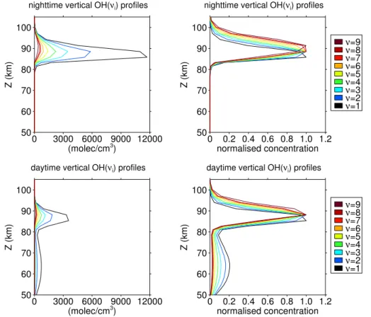
For the first part of this study we will discuss some general features of simulated verti-cal OH* profiles. Figure 1 shows two examples of vertiverti-cal vibrational populations with one referring to nighttime conditions (upper panels) and the other referring to daytime

20

conditions (lower panels). In accordance with von Savigny et al. (2012) the nighttime vibrational populations form single peak profiles that are shifted upwards with respect to their vibrational state (upper right panel). Moreover, the vertical shift between diﬀ er-ent vibrational populations is more pronounced above their peak altitudes. Based on a sensitivity study, von Savigny et al. (2012) relate this asymmetry in the vertical shifts

25

(10)

ACPD

14, 1239–1285, 2014

Title Page

Tables Figures

◭ ◮

Back Close

Full Screen / Esc

Discussion

P

a

per

|

D

iscussion

P

a

per

|

Discussion

P

a

per

|

Discuss

ion

P

a

per

|

constant. With respect to our daytime example, we can find a secondary peak that is particularly pronounced for lower vibrational states. If we limit our comparison to the main peak of day- and nighttime profiles, we can see that absolute nighttime concen-trations generally exceed daytime concenconcen-trations. This is something we would expect, because the loss of O3due to photodissociation during sunlit conditions is directly im-5

pacting Reaction (R1). Interestingly, absolute daytime concentrations appear to exceed nighttime concentrations, where they form the secondary peak at about 62 km. A sim-ilar daytime profile structure is shown in a model study of Funke et al. (2012), which is also accounting for non-LTE conditions in its algorithms. They argue that the lower daytime peak results from the larger daytime H abundances, which we can also find in

10

the SD-WACCM 4 profiles.

In the following, we will mainly focus on nighttime OH*, because the relatively low abundances of daytime OH* and the large Rayleigh scattering background make OH* daytime observations very diﬃcult.

3.2 OH* concentrations and emission peak altitudes

15

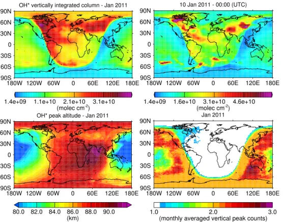
Before we will address the temporal evolution of individual OH(ν) vertical profiles, we first consider the sum over all vibrational OH(ν=1, 2,. . ., 9) profiles. Figure 2 shows an example of simulated OH*, where the upper left panel refers to a monthly mean and the upper right panel refers to an arbitrary daily sample within the same monthly mean to illustrate some of its fine scale features.

20

One can clearly see the sharp day/night transition from low to high OH* concen-trations in both panels. Interestingly, for the daily sample we can find at mid-southern latitudes some striking synoptic scale daytime features of exceptionally high OH* centrations similar to nighttime concentrations. These features still remain, if we con-sider individual vibrational levels (not shown) and can persist for a few days. Similar

25

(11)

ACPD

14, 1239–1285, 2014

Title Page

Tables Figures

◭ ◮

Back Close

Full Screen / Esc

Discussion

P

a

per

|

D

iscussion

P

a

per

|

Discussion

P

a

per

|

Discuss

ion

P

a

per

60 km. Because of our emphasis on nighttime concentrations, we keep these features as a note.

For nighttime OH*, we can see a general eastward decrease in the vertically inte-grated concentrations. We can find a similar trend for all months throughout the year, but the high OH* concentrations ranging from central Asia to Siberia appear to be

5

a special feature of this month.

According to our previous discussion, we can interpret the eastward decrease in OH* concentrations as a nighttime decrease by converting the longitudes in Fig. 2 to local times. In addition to the decreasing nighttime trend, we can also find enhanced OH* concentrations at the equatorial regions, which minimise at around±30◦. This

latitudi-10

nal structure is consistent with the study of Marsh et al. (2006) and other observational studies stated therein.

Previous studies based on observations made with the high-resolution Doppler im-ager (HRDI) instrument and the Wind Imaging Interferometer (WINDII) instrument on-board the upper atmosphere research satellite (UARS) revealed that the peak altitude

15

of the OH* emission layer increases with decreasing integrated emission rate, which is explained by the vertical motions associated with tides or other processes (see Cho and Shepherd, 2006; Liu and Shepherd, 2006 and references therein). To check as to whether our simulated vertical OH* profiles are consistent with this finding, we de-termine the peak altitude of each profile by weighting the geometric heights with the

20

vertical OH* number density profiles. Based on this method, the lower left panel of Fig. 2 shows the monthly average of our weighted peak altitudes. If we exclude the region of enhanced OH* concentrations above central Asia and Siberia, we can see that peak altitudes increase over the course of the night by up to 4 km. In contrast, the area of enhanced OH* concentrations above central Asia and Siberia shows a

pro-25

(12)

ACPD

14, 1239–1285, 2014

Title Page

Tables Figures

◭ ◮

Back Close

Full Screen / Esc

Discussion

P

a

per

|

D

iscussion

P

a

per

|

Discussion

P

a

per

|

Discuss

ion

P

a

per

|

important aspect with regard to the OH* profile shape. If we remember the double peak structure of the daytime OH* profile according to Fig. 1, in this case the determination of peak altitudes by weighting the whole vertical profile would appear less meaning-ful. In general, the existence of multiple peak structures in the vertical OH* profiles would complicate the comparison between diﬀerent OH(ν)* layers, thus, aﬀecting our

5

study on the OH* quenching process in the following sections. However, according to our nighttime example in Fig. 1 we may assume that nighttime OH* profiles generally follow a single peak shape. To validate this assumption, we have counted the number of local maxima of each vertical OH* number density profile that occurs above 50 km altitude. Furthermore, local maxima must have amplitudes of at least 10 % with

re-10

spect to the largest peak of the vertical OH* number density profile. Based on these counting rules, the lower right panel in Fig. 2 shows the monthly average of daily peak counts. As we can see, indeed the nighttime vertical OH* profiles mainly consist of sin-gle peaks, hence, we should expect no significant interference with our peak altitude determination method during the nighttime. Only around the early evening hours at mid

15

and high northern latitudes, occasionally multiple peak structures appear in the vertical OH* profiles but the overall contribution remains low. Furthermore, we find the same dominating single peak structure for the other months of our dataset (not shown). In addition to the validation of our assumption on the single peak shape of nighttime OH* profiles, this finding could also have an interesting implication for observational studies

20

that report noticeable amounts of complex multiple peak structures in the vertical OH* VER profiles during nighttime (e.g. Melo et al., 2000 report such structures for up to 25 % of their examined WINDII profiles). Because these complex structures can either result from vertical or lateral inhomogeneities, the dominant single peak shape we find in the vertical OH* WACCM profiles would suggest the latter case.

25

3.3 Vertical displacements of OH(ν)

(13)

ACPD

14, 1239–1285, 2014

Title Page

Tables Figures

◭ ◮

Back Close

Full Screen / Esc

Discussion

P

a

per

|

D

iscussion

P

a

per

|

Discussion

P

a

per

|

Discuss

ion

P

a

per

above the peak altitudes. We further refine our study by focusing on two diﬀerent vibra-tional states in the following.

To allow a later comparison with SABER VER measurements, we select the OH(9) and OH(5) layers, because they both contain emissions, which can be observed by the 1.6 and 2.0 µm SABER channels separately. Ideally, one must consider that each

5

SABER channel captures a mixture of emissions that belong to two different transition bands. However, because the difference in vibrational levels between each transmis-sion is limited to∆ν=1, we assume that we can neglect the effect of profile mixing for each channel, if we are interested in the relative vertical displacement between both (mixed) OH* profiles.

10

In order to determine the vertical displacement between two OH* layers, we can subtract their corresponding (profile) weighted geometric altitudes from each other. On the other hand, our case example of a vertical OH* profile according to Fig. 1 illustrates that the vertical spread between diﬀerent OH(ν) layers increases with height due to the increase in the eﬀective O quenching that results from the steep vertical

15

gradient of O concentrations. For our study on the response of the relative distance between the OH(9) and OH(5) layers to changes in O concentrations, this seems to favor a comparison between the upper parts of both layers. To account for this, we can interpolate the altitudes, where both OH(ν) number density/VER profiles have dropped by a factor of 0.5 relative to the OH* number density/VER profile peak value, which

20

we will refer to as the Half Width at Half Maximum (HWHM) in the following. However, as we will soon discuss, this criterion to determine the vertical displacement between both layers is also highly sensitive to relative changes in the profile shapes, which could aﬀect the correlation with changes in atomic oxygen. On the other hand, changes in the relative layer widths should have a less pronounced eﬀect for the weighted peak

25

(14)

ACPD

14, 1239–1285, 2014

Title Page

Tables Figures

◭ ◮

Back Close

Full Screen / Esc

Discussion

P

a

per

|

D

iscussion

P

a

per

|

Discussion

P

a

per

|

Discuss

ion

P

a

per

|

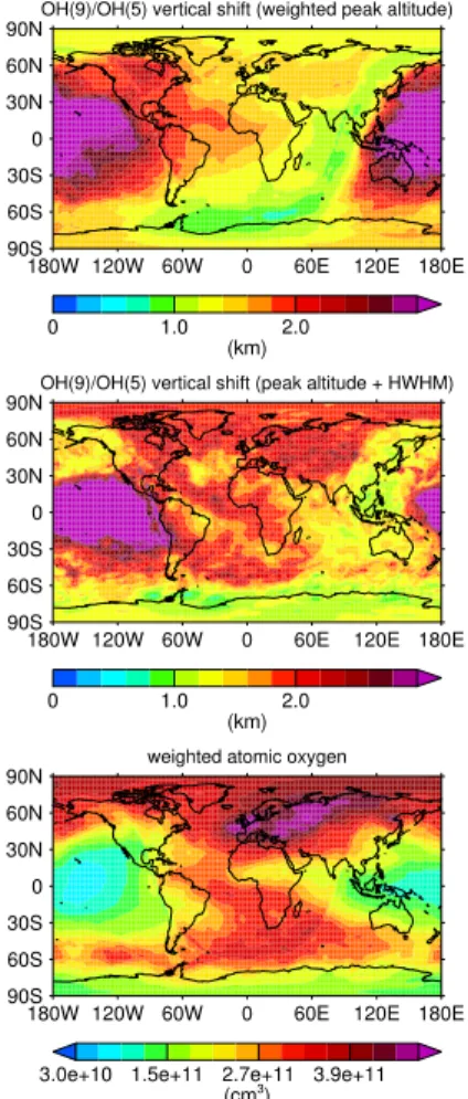
Fig. 3 shows determined values of vertical shifts∆Z_9,5 between simulated OH* pro-files for the same temporal average as being considered in Fig. 2. For the vertical shift between weighted peak altitudes, we can find a general decrease in∆Z_9,5values over the course of the night. In contrast, the nighttime evolution of∆Z_9,5 at the upper part of the OH* layer is more complex. To relate the nighttime evolution of vertical shifts

5

with changes in O, we choose to calculate O concentrations by weighting their vertical profiles with the OH(9) concentrations in Fig. 3. We will also address other methods to account for temporal changes in O concentrations at the end of this section.

By comparison with the lower panel in Fig. 3, we can see that the diurnal evolution of weighted O can hardly explain the rather monotonic decrease in nighttime∆Z_9,5for

10

weighted peak altitudes. The situation still remains diﬃcult when considering∆Z_9,5for HWHM shifted peak altitudes. If we focus again on north-eastern latitudes, we can see a striking maximum of weighted O concentrations. The decrease in OH* layer altitudes in the same region could reflect an enhanced downward transport that is driven by strong advection from lower latitudes according to Smith et al. (2011). In comparison,

15

the response in∆Z_9,5for HWHM shifted peak altitudes is not as pronounced for this re-gion, though values are relatively high. In addition, the variability in∆Z_9,5is larger than for weighted O concentrations, hence, the diurnal response to O quenching appears to be less evident than initially expected.

To gain a better understanding of the actual impact of O quenching on the diurnal

20

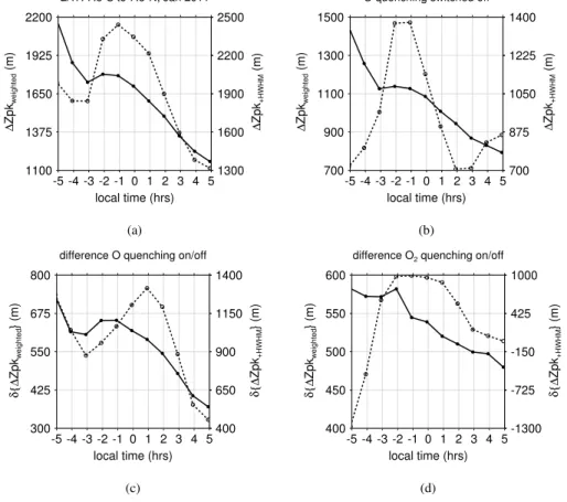
evolution of∆Z_9,5, we investigate its sensitivity by creating an additional model run, where we switch oﬀthe O quenching term in Eq. (1) and compare the resulting∆Z_9,5 values between both model runs. This is done in Fig. 4, where panel (a) shows re-sulting vertical shifts from a model run including all quenching rate terms in Eq. (2) and panel (b) shows the result for the same model run with deactivated O quenching.

25

(15)

ACPD

14, 1239–1285, 2014

Title Page

Tables Figures

◭ ◮

Back Close

Full Screen / Esc

Discussion

P

a

per

|

D

iscussion

P

a

per

|

Discussion

P

a

per

|

Discuss

ion

P

a

per

between a model run including all quenching rate terms and a model run with deacti-vated O₂quenching in panel (d). Because of its rather ineﬃcient quenching capability, we skip a similar comparison for the N2quenching.

For the full quenching case, we can find a local maximum in vertical shifts close to

−1 h LST in panel (a) of Fig. 4. This maximum is significantly enhanced for the HWHM

5

shifted peak altitudes. If we switch oﬀthe O quenching, we can clearly see that vertical shifts have noticeably decreased for both altitude definitions according to panel (b). However, certain similarities persist with respect to the full quenching model run.

For peak shifts calculated from weighted peak altitudes, we can still find a local maximum close to−1 h, which decrease by about 330 m until+5 h. By comparison, the

10

decrease is about 630 m for the full quenching case, i.e. the diurnal decrease in peak shifts increases by a factor of about 1.9 due to the activated O quenching. Interestingly, the deactivation of O2quenching is also significantly aﬀecting the peak shifts according

to panel (d). However, despite the change of peak shifts by up to 580 m due to the deactivation of O₂quenching according to panel (d), the diﬀerence to the full quenching

15

model run varies only by about 50 m between −1 h and +5 h, which is rather small compared to the eﬀect of O quenching.

For the HWHM shifted peak altitudes, the diﬀerences are generally larger when switching the O quenching on and oﬀ. Moreover, the response to O quenching in Fig. 4c is less coherent with the diurnal evolution of vertical shifts without O quenching

20

in Fig. 4b. For early (<−3 h) and late (>+3 h) LST, the trend is opposite in both cases. In addition, the strongest impact from O quenching is shifted from −1 h to +1 h LST. This indicates a potential diﬃculty for our attempt to correlate the diurnal evolution in vertical shifts with that of atomic oxygen, because the diurnal variability of about 670 m in Fig. 4b is very close to the diurnal variability of about 790 m in Fig. 4c, hence we fail

25

to differentiate between the process of O quenching and other processes in Fig. 4b be-cause of their similar magnitudes. Another difficulty arises with respect to O₂quenching according to Fig. 4d. The activation of O2 quenching can lead to differences in

(16)

ACPD

14, 1239–1285, 2014

Title Page

Tables Figures

◭ ◮

Back Close

Full Screen / Esc

Discussion

P

a

per

|

D

iscussion

P

a

per

|

Discussion

P

a

per

|

Discuss

ion

P

a

per

|

variability is rather constant in the periods between−2 h to+1 h and+3 h to +5 h, the decrease in vertical shifts between these periods is about 650 m, which is significantly larger than for O quenching during the same period.

Keeping in mind the revealed diﬃculties in our attempt to relate vertical shifts with O quenching, we also have to address the actual method to determine the strength of O

5

quenching. The simplest method is to look at the diurnal evolution of O at a constant height level. However, this method neglects any changes of O concentrations that arise from the vertical motion of the entire OH* layer. To account for this, we may determine the O concentration at a fixed reference point of the OH* layer. Again, this method is still rather simple, because the O quenching is not constrained to a fixed point at the

10

OH* layer. Similar to our example in Fig. 3, we may account for the entire quenching of OH* with O by weighting the vertical O profile with the OH* profile. From all of these approaches, we present their diurnal evolutions in Fig. 5. In addition, we also included the corresponding diurnal evolution of molecular oxygen in the same figure. To allow a better comparison between diﬀerent methods, we subtracted the minimum value of

15

each curve and denote their values in the legend. If we neglect these offsets, we can still see noticeable differences between different methods, hence the selection between these approaches can lead to different correlations with observed vertical shifts.

For atomic oxygen, we find a single maximum close to −1 h LST according to the fixed 0.241 Pa pressure level (approx. 90 km altitude). If we neglect the−5 h LST, which

20

is close to twilight conditions, O concentrations seem to follow peak shifts based on weighted peak altitudes in panel (c) of Fig. 4. However, the observed response at+1 h for HWHM shifted peak altitudes is not reflected at a constant pressure level. If we interpolate O concentrations at a fixed point of the OH* layer, we find an additional diurnal response around+1 h LST. Although this matches the observed response in

25

vertical shifts based on HWHM shifted peak altitudes in panel (c) of Fig. 4, it is not as pronounced. This situation also remains, if we consider weighted O concentrations.

For molecular oxygen, we find two diﬀerent situations. On the one hand O2

(17)

ACPD

14, 1239–1285, 2014

Title Page

Tables Figures

◭ ◮

Back Close

Full Screen / Esc

Discussion

P

a

per

|

D

iscussion

P

a

per

|

Discussion

P

a

per

|

Discuss

ion

P

a

per

the OH(9)/OH(5) profiles show a systematic decrease over the course of the night. Moreover, the diurnal gradient is steeper with respect to the lower OH(5) layer. On the other hand, the diurnal variability of O2 concentrations interpolated at HWHM shifted

positions (red lines) is relatively small. In addition, the diurnal variability of O₂ at the 0.241 Pa level is also relatively small. Apparently, the observed larger magnitude of

5

diurnal O2 changes according to the first two definitions must be connected to the

in-creasing O₂ concentrations with decreasing altitudes. By comparison with the diurnal variability of vertical shifts according to panel (d) of Fig. 4, the systematic decrease with respect to weighted peak altitudes is accompanying the diurnal decrease of O2

concentrations according to the first two definitions. However, none of our O₂

concen-10

tration definitions is capable of reflecting the drastic changes in vertical shifts based on HWHM shifted peak altitudes according to panel (d) of Fig. 4.

In addition to our example close to solstice conditions, we also performed similar tests with respect to equinox conditions, where the amplitude of the migrating diurnal tide maximises. However, despite the larger diurnal variability in O abundances, we

15

encounter similar problems to relate changes in peak shifts with changes of the O and O₂quenching species.

So far we must conclude that we cannot explain the diurnal variability in vertical shifts between the OH(9)/OH(5) layers with the diurnal variation of the two most im-portant quenching species only. In particular this applies for vertical shifts calculated

20

from HWHM shifted peak altitudes, despite the more pronounced vertical spread be-tween diﬀerent vibrational populations at this part. In this context we must note that the latter definition is more sensitive to changes in the profile shape of both vertical OH(ν) populations. While changes in the profile shape can be induced via modulating the abundances of quenching species, the variability of the H+O3 profiles according 25

(18)

ACPD

14, 1239–1285, 2014

Title Page

Tables Figures

◭ ◮

Back Close

Full Screen / Esc

Discussion

P

a

per

|

D

iscussion

P

a

per

|

Discussion

P

a

per

|

Discuss

ion

P

a

per

|

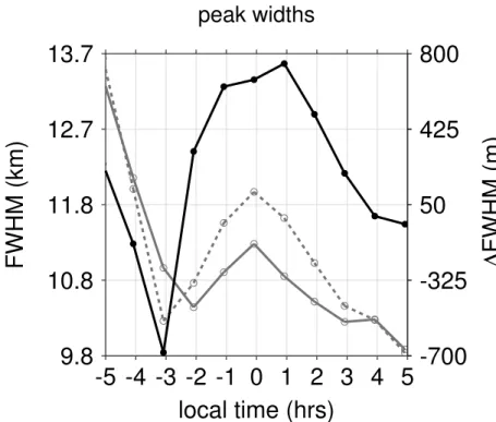
pronounced changes with a largest diﬀerence between both FWHM values around+1 h LST. According to panels (c) and (d) of Fig. 4, the largest response to HWHM shifted peak altitudes appears at the same time, indicating the sensitivity of this parameter to relative changes of peak layer widths.

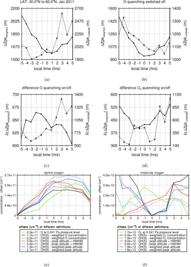
In addition to this equatorial example, we briefly do a similar comparison for the

lat-5

itudinal range between 30◦N and 60◦N, which encloses the strong enhancement of atomic oxygen in the second half of the night. Similar to Fig. 4, diﬀerent model runs are shown in Fig. 7. As expected, we can see a strong increase of nighttime O for all definitions according to panel (e) of Fig. 7. This time, it is rather the peak shift based on HWHM shifted peak altitudes, which seems to follow the nighttime trend in atomic

10

oxygen. According to Fig. 8, we find again a strong coherence with the relative change in OH(9)/OH(5) peak layer widths. With respect to the deactivation of O2 quenching

according to panel (d) of Fig. 7, it is worth noting that the temporal variability based on weighted peak altitudes is about 140 m, which is more than two times larger com-pared to the equatorial example. If we consider the diurnal evolution of O2 according 15

to panel (f), different definitions lead to quite different results. Furthermore, all defini-tions show systematic differences with respect to the temporal evolution of peak shifts based on weighted peak altitudes according to panel (d). For the peak shifts based on HWHM shifted peak altitudes (same panel), we find again some substantial changes when switching offthe O₂ quenching. In general the response of the peak definition

20

based on HWHM shifted peak altitudes shows a strong coherence with the diurnal evolution of relative changes in OH(9)/OH(5) peak widths shown in Fig. 8.

3.4 SABER

Before we will discuss the diurnal evolution of vertical VER profiles measured by SABER, we must address two important issues that would aﬀect a direct

compari-25

(19)

ACPD

14, 1239–1285, 2014

Title Page

Tables Figures

◭ ◮

Back Close

Full Screen / Esc

Discussion

P

a

per

|

D

iscussion

P

a

per

|

Discussion

P

a

per

|

Discuss

ion

P

a

per

yaw-cycle, but this would also smear out some interesting features shown before, such as the discussed enhanced OH* concentrations at north-eastern latitudes. Further-more, our conversion from longitudes to LST assumes that any zonal variability reflects a purely time-dependent process. However Xu et al. (2010) found evidence of notice-able non-migrating tides from SABER observations at lower latitudes, which would

vi-5

olate this assumption. It is for these reasons that we do not intend a direct comparison between SABER and SD-WACCM4 in this section, thus, we will mainly focus on the general relationship between vertical shifts between OH* VER profiles measured by the 1.6 and 2.0 µm SABER channels and changes in derived O concentrations.

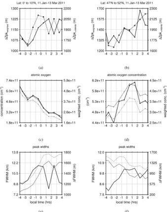
Figure 9a and c show derived peak shifts and O concentrations for the equatorial

10

region between 0◦ and 10◦N. Similar to our model study, we determined O concentra-tions based on diﬀerent methods. Here, we limit our consideration to O concentrations derived at 90 km altitude and O concentrations weighted with the vertical OH* VER profiles according to both SABER channels. As with our model results, the comparison between peak shifts and O concentrations hardly reveal any consistent relationship.

15

The same also applies for the mid-latitudinal example in Fig. 9b and d, which is sug-gesting again that the diurnal variability of the vertical peak shifts is mainly driven by the diurnal variability of the H and O3profiles.

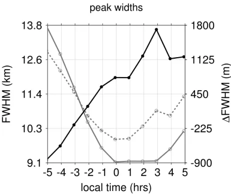
Similar to our model results, we find a strong variability in the diurnal evolution of the OH* peak widths according to Fig. 9e and f. In particular for the equatorial example, the

20

(20)

ACPD

14, 1239–1285, 2014

Title Page

Tables Figures

◭ ◮

Back Close

Full Screen / Esc

Discussion

P

a

per

|

D

iscussion

P

a

per

|

Discussion

P

a

per

|

Discuss

ion

P

a

per

|

4 Seasonal evolution of OH* layer shifts

4.1 Model study

We leave our case example of the previous section and will now focus on the full year period of simulated OH* starting from April 2010. Similar to the previous section, we will investigate to what extent the seasonal variability of∆Z_9,5peak shifts is aﬀected by

5

the quenching of OH* with molecular and atomic oxygen.

With respect to equatorial latitudes, the diurnal migrating tide is an important pro-cess aﬀecting the OH* airglow and ambient temperatures (Shepherd et al., 2006). Many studies have reported evidence of a semi-annual oscillation in airglow obser-vations that is associated with the large seasonal changes in the tidal amplitude. For

10

instance, Marsh et al. (2006) present a pronounced semi-annual oscillation in SABER OH* VER measurements at equatorial latitudes. A similar seasonality was also recently shown for OH* VER measurements from SCIAMACHY (SCanning Imaging Absorption spectroMeter for Atmospheric CHartographY) by von Savigny and Lednyts’kyy (2013). In addition, a semi-annual oscillation was also reported from HRDI observations (Yee

15

et al., 1997) and ISIS-2 observations (Cogger et al., 1981) of the O(1S) green line. Be-cause the vertically integrated O concentration should be proportional to the integrated OH* VER (see Eq. 2 in Mlynczak et al., 2013), the same observed seasonal variabil-ity could also apply for the ∆Z_9,5 peak shift. Indeed, the study of von Savigny and Lednyts’kyy (2013) finds evidence of the same semi-annual oscillation between

SCIA-20

MACHY measurements of O abundances derived from the O(1S) green line and the vertical displacement between the OH(3-1)/OH(6-2) transmission bands at equatorial latitudes.

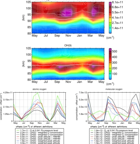
Following-up these findings, Fig. 10 shows 1 yr of SD-WACCM4 O concentrations together with derived OH(9) concentrations at equatorial latitudes in the LST range

25

(21)

ACPD

14, 1239–1285, 2014

Title Page

Tables Figures

◭ ◮

Back Close

Full Screen / Esc

Discussion

P

a

per

|

D

iscussion

P

a

per

|

Discussion

P

a

per

|

Discuss

ion

P

a

per

concentrations (not shown). In addition, we can find similar enhancements in atomic oxygen around both equinoxes, which again is consistent with the previously suggested proportionality between O and OH* concentrations. Interestingly, a similar semi-annual oscillation also exists for O₂concentrations according to the lower right panel of Fig. 10 except for O2concentrations at the constant 0.241 Pa pressure level. This indicates the 5

important role of the seasonal variability of the eﬀective O2quenching process, which in

turn can significantly aﬀect the vertical OH* structure according to the previous section. If we consider the resulting ∆Z_9,5 peak shifts based on weighted peak altitudes in Fig. 11, we can also find an enhancement around both equinoxes, but a less dis-tinct minimum close to the December solstice. According to the panel (b) in Fig. 11,

10

the equinoctial enhancements in∆Z_9,5 peak shifts still persist, if we switch oﬀ the O quenching, however, the∆Z_9,5maximum around the December solstice is contrasting the temporal evolution of O concentrations. The semi-annual oscillation in∆Z_9,5 peak shifts is seen more clearly, if we subtract model runs with and without O quenching from each other as shown in panel (c). The comparison between both model runs

indi-15

cates that the semi-annual amplitudes enhance by a factor of about 2.5, if we consider O quenching in our OH* model. For the deactivation of quenching with O₂, the impact on the seasonal evolution of∆Z_9,5peak shifts is smaller with respect to weighted peak altitudes according to panel (d). For instance, the peak shift variation between August and October is about 200 m for switching O quenching on and oﬀ, which is about two

20

time larger compared to switching the O2quenching on and oﬀ. With respect to HWHM

shifted peak altitudes, again a significant seasonal variability exists in panel (d). In addition to∆Z_9,5 peak shifts and O concentrations, we find another semi-annual oscillation in the weighted OH* peak altitudes (see panel (e) of Fig. 11) in accordance with other studies (e.g. see Shepherd et al., 2006, and von Savigny and Lednyts’kyy,

25

(22)

ACPD

14, 1239–1285, 2014

Title Page

Tables Figures

◭ ◮

Back Close

Full Screen / Esc

Discussion

P

a

per

|

D

iscussion

P

a

per

|

Discussion

P

a

per

|

Discuss

ion

P

a

per

|

strong vertical gradient in O concentrations at OH* altitudes, the seasonal variabil-ity in OH* peak altitudes induces a semi-annual oscillation that should be associated with stronger O quenching around each solstice. Despite the opposing eﬀect between the vertical and temporal change in O concentrations, the temporal variability appears to dominate the seasonal variability in the O quenching according to Fig. 11. On the

5

other hand, the large enhancement in peak altitudes around January associated with larger O quenching could explain the less distinct minimum in peak shifts around the solstice period. We should note that an anti-phase relation also exists between OH* al-titudes and O2concentrations. Because of the still relatively constant O2VMR at these

altitudes, absolute concentrations are modulated via temperature/pressure changes.

10

Interestingly, the anti-phase relation to OH* altitudes rather seems to contribute to the observed semi-annual oscillation in O2in contrast to O because of the increasing O2

density with decreasing altitudes. In addition, the temperature changes due to the mod-ulation of the amplitude of the migrating diurnal tide, is also aﬀecting the absolute O₂ concentrations.

15

With respect to the HWHM shifted peak altitudes, it is more diﬃcult to find a clear seasonal dependency according to Fig. 11. By subtracting our OH* model runs with and without O quenching from each other, two distinct enhancements remain around both equinoxes. In particular the change in∆Z_9,5 peak shifts from summer-solstice to the mid of October is about two times larger, if we consider shifted instead of weighted

20

peak altitudes. However, these enhancements are almost constrained to a single month each, i.e. they follow a more pulse like response rather than a smooth harmonic oscil-lation. Again, the comparison with the relative change of peak layer widths according to panel (f) of Fig. 11 shows strong changes during the same months, but also some diﬀerences remain with respect to the seasonal variability according to panel (a).

25

(23)

ACPD

14, 1239–1285, 2014

Title Page

Tables Figures

◭ ◮

Back Close

Full Screen / Esc

Discussion

P

a

per

|

D

iscussion

P

a

per

|

Discussion

P

a

per

|

Discuss

ion

P

a

per

independent) meridional circulation. However, if we consider the global distribution of vertically integrated OH* in Fig. 2, it is obvious that the nighttime period rapidly de-creases during the summer season at high latitudes. Apparently, the inclusion of peri-ods with daytime OH* would introduce a significant annual oscillation in OH* concentra-tions that is independent of the meridional circulation. Hence, we preferably select a

lo-5

cal time within a latitudinal range that is not aﬀected by sunlit photochemistry through-out the year to investigate the influence of the meridional circulation on OH* concentra-tions. Accordingly, we choose the latitudinal range from 50◦S to 55◦S at 00:00 UTC in Fig. 12. For the annual variability of atomic oxygen we can see a pronounced maximum in O concentrations at the Northern Hemisphere around January 2011, which is shortly

10

followed by a similar enhancement at the Southern Hemisphere in February 2011. The reported 60◦S OH* maximum around May from Marsh et al. (2006) does not fit with the SD-WACCM4 enhancement in O concentration. This could indicate a special case with respect to the vertical transport component of the meridional circulation in 2011, but due to our limited dataset and our general emphasis on O quenching the final

15

assessment of this question already exceeds the scope of this paper.

In contrast to our comparison in Fig. 11, the impact of O (and O₂) quenching seems to play a minor role for the variability in∆Z_9,5peak shifts at higher latitudes. This result might be surprising, in particular when considering the relatively constrained periods with high O concentrations in both hemispheres. With respect to weighted peak

alti-20

tudes, the response in∆Z_9,5peak shifts to changes in O concentrations only becomes visible when subtracting the model runs with and without O quenching from each other. For instance, we can find two enhancements in ∆Z_9,5 peak shifts in November and February and a minimum around August in the SH, which fits to the seasonal change in O concentrations according to Fig. 12. However, the seasonal variability in ∆Z_9,5 25

(24)

ACPD

14, 1239–1285, 2014

Title Page

Tables Figures

◭ ◮

Back Close

Full Screen / Esc

Discussion

P

a

per

|

D

iscussion

P

a

per

|

Discussion

P

a

per

|

Discuss

ion

P

a

per

|

definition appears to be highly aﬀected by the relative change of peak layer widths, showing a semi-annual oscillation around both equinox.

4.2 Comparison with SABER

We will now focus on the seasonal variability of the vertical shifts between OH* profiles according to SABER VER measurements within the same−1 h to 0 h LST bin that is

5

also used for our model study. Figure 14 shows the seasonal variability of equatorial OH* peak shifts and O concentrations, that are both derived from VER measurements of the SABER 1.6 and 2.0 µm channels for the period from January 2009 to Decem-ber 2011. Figure 15 gives a similar example for high latitudes.

By comparing both equatorial latitude bins, a semi-annual oscillation in OH* weighted

10

O concentrations is much more pronounced for the 0◦ to 10◦S bin than for the 0◦ to 10◦N bin, where an apparent annual component dominates. A similar situation applies for the O concentrations at 90 km altitude. Interestingly, a pronounced semi-annual os-cillation is apparent for both equatorial latitude bins in terms of peak shifts between both OH* SABER profiles. Even though the semi-annual amplitude of peak shifts based on

15

weighted peak altitudes is larger for the 0◦ to 10◦S bin, it is worth noting that a semi-annual oscillation persists for the 0◦to 10◦N latitude bin despite the dominating annual component of the corresponding atomic oxygen oscillation. This again indicates that further processes must be taken into account for the seasonal variation of OH* peak shifts. Furthermore, the strong coherence between the relative modulation of VER

pro-20

file widths and peak shifts based on shifted peak altitudes (compare dashed line of upper panels with solid black line of lower panels) confirms the strong relationship be-tween both parameters that has also been previously observed in this study.

The mid-latitudinal example in Fig. 15 is rather dominated by an annual oscillation through all parameters. In particular the relative change between the VER profile widths

25

(25)

ACPD

14, 1239–1285, 2014

Title Page

Tables Figures

◭ ◮

Back Close

Full Screen / Esc

Discussion

P

a

per

|

D

iscussion

P

a

per

|

Discussion

P

a

per

|

Discuss

ion

P

a

per

a similar strong increase shortly after the turn over of the meridional circulation in February for the SABER observations. However, the larger averaging time due to our constraint of one yaw cycle could smooth out such an event.

5 Summary and conclusion

By combining a quenching model with a state-of-the-art 3-D chemical climate model

5

(SD-WACCM4), this study has investigated the temporal evolution of the OH* species with special emphasis on the impact of the quenching process due to O and O₂. Based on a monthly case example, this model approach confirms general features of the global distribution of OH* that have been reported by previous observational and theo-retical studies, in summary:

10

– The diurnal decrease in nighttime OH* concentrations.

– The inverse relationship between integrated OH* columns and OH* peak altitudes.

– The prominence of single peak OH* profiles during nighttime.

The latter point suggests that complex structures, which have been observed in verti-cal OH* VER profiles during nighttimes, are caused more likely by lateral rather than

15

vertical inhomogeneities in the distribution of OH*.

Even though, the main focus of this study is on the nighttime, some interesting SD-WACCM4 based daytime features were revealed in addition, i.e.:

– Daily profiles show more complex structures.

– Pronounced synoptic scale features of large daytime OH* abundances exist.

20

(26)

ACPD

14, 1239–1285, 2014

Title Page

Tables Figures

◭ ◮

Back Close

Full Screen / Esc

Discussion

P

a

per

|

D

iscussion

P

a

per

|

Discussion

P

a

per

|

Discuss

ion

P

a

per

|

abundances are significantly aﬀected by sunlit photochemistry. Moreover, these fea-tures are most prominent during solstice conditions and mainly constrained to sum-mer hemispheric mid-latitudes. A further investigation of these systematic features is needed.

In the next part of this study, the quenching of OH* with O and O2 was investigated 5

by creating model runs with:

– Full quenching.

– Deactivated O quenching.

– Deactivated O2quenching.

From these model runs, vertical displacements between the OH(9) and OH(5) layers

10

are determined and compared with abundances of the O and O₂ quenching species. We find that despite the deactivation of O and O2 quenching, a noticeable

tempo-ral variability remains in the vertical OH(9)/OH(5) displacements in both cases, which must be attributed to the natural variability in the H and O₃ profiles that lead to the production of OH*. For the diurnal variability, this factor is even dominating in both,

15

SD-WACCM4 based simulations and SABER observations, hence we fail to find a sig-nificant correlation between the vertical OH(9)/OH(5) displacements and the eﬀective quenching with either O or O2. However, the situation has changed for the seasonal

evolution at the equatorial regions. In this case, a pronounced semi-annual oscillation exists in the vertical displacement of the simulated OH(9)/OH(5) layers, which we also

20

find in the OH* VER measurements from SABER. In addition, our study reveals that a similar oscillation also exists for the absolute O and O2concentrations at OH* layer

altitudes, thus, demonstrating the importance of the quenching process to the revealed semi-annual oscillation in the vertical OH* profile structure. While previous studies have already outlined the eﬀect of O quenching to the OH* profile, the systematic impact of

25

(27)

ACPD

14, 1239–1285, 2014

Title Page

Tables Figures

◭ ◮

Back Close

Full Screen / Esc

Discussion

P

a

per

|

D

iscussion

P

a

per

|

Discussion

P

a

per

|

Discuss

ion

P

a

per

Gattinger et al., 2013 and references therein). In general, despite the less eﬃcient O₂ quenching compared to O quenching, we must conclude from our study, that the higher absolute abundance of O2 is compensating this, in particular at the lower part of the

OH* layer.

In addition to the semi-annual oscillation of the two most important OH* quenching

5

species, we also find a remaining similar oscillation in the model runs with deactivated quenching parameters. This implies that the natural variability of H and O₃ still plays a noticeable role for the seasonal variability of the vertical OH* structure. Therefore, we conclude from our model results that the observed semi-annual oscillation cannot be entirely explained by the quenching process alone.

10

Because of the manifold of transition bands being observed by diﬀerent ground-based instruments, a thorough understanding of the driving processes of the variability of OH* emission altitudes is crucial for the intercomparison and interpretation of long-term data sets. This in particular applies for the studying of mesopause temperature trends by means of OH* rotational temperature measurements (see Beig et al., 2003;

15

Beig, 2011, for a comprehensive review on this topic). A future model study, which includes a multiyear analysis of the features that have been discussed here, would fur-ther contribute to a better quantitative understanding of the systematic biases between diﬀerent observational long-term studies.

Acknowledgements. This work was in part supported by the Ernst-Moritz-Arndt-University of

20

Greifswald. Further support was granted by the German Research Foundation (Deutsche Forschungsgemeinschaft, DFG) under project PA 1714/4-2. We thank I. McDade, York Univer-sity, Toronto, for the provision of the initial quenching algorithm, which we have adapted in the frame of this study. We also thank R. R. Garcia and D. E. Kinnison, NCAR Boulder, for providing the SD-WACCM4 data to us, which have been a crucial component of this study. In addition,

25

(28)

ACPD

14, 1239–1285, 2014

Title Page

Tables Figures

◭ ◮

Back Close

Full Screen / Esc

Discussion

P

a

per

|

D

iscussion

P

a

per

|

Discussion

P

a

per

|

Discuss

ion

P

a

per

|

References

Adler-Golden, S.: Kinetic parameters for OH nightglow modeling consistent with recent labora-tory measurements, J. Geophys. Res., 102, 19969–19976, 1997. 1241, 1270

Bates, D. R. and Nicolet, M.: The photochemistry of atmospheric water vapor, J. Geophys. Res., 55, 301–327, 1950. 1241

5

Beig, G.: Long-term trends in the temperature of the mesosphere/lower thermosphere region: 2. Solar response, J. Geophys. Res., 116, A00H12, doi:10.1029/2011JA016766, 2011. 1265 Beig, G., Keckhut, P., Lowe, R. P., Roble, R. G., Mlynczak, M. G., Scheer, J., Fomichev, V. I., Oﬀermann, D., French, W. J. R., Shepherd, M. G., Semenov, A. I., Remsberg, E. E., She, C. Y., Lübken, F. J., Bremer, J., Clemesha, B. R., Stegman, J., Sigernes, F., and

10

Fadnavis, S.: Review of mesospheric temperature trends, Rev. Geophys., 41, 1015–1055, doi:10.1029/2002RG000121, 2003. 1265

Cho, Y.-M. and Shepherd, G.: Correlation of airglow temperature and emission rate at Res-olute Bay (74.86◦N), over four winters (2001–2005), Geophys. Res. Lett., 33, L06815, doi:10.1029/2005GL025298, 2006. 1249

15

Cogger, L. L., Elphinstone, R. D., and Murphree, J. S.: Temporal and latitudinal 5577 A airglow variations, Can. J. Phys., 59, 1296–1307, 1981. 1258

Dodd, J. A., Lipson, S. J., Lowell, J. R., Armstrong, P. S., Blumberg, W. A. M., Nadile, R. M., Adler-Golden, S. M., Marinelli, W. J., Holtzclaw, K. W., and Green, B. D.: Analysis of hy-droxyl earthlimb airglow emissions: kinetic model for state-to-state dynamics of OH (v,N), J.

20

Geophys. Res., 99, 3559–3585, 1994. 1241

Funke, B., López-Puertas, M., García-Comas, M., Kaufmann, M., Höpfner, M., and Stiller, G.: GRANADA: a Generic RAdiative traNsfer AnD non-LTE population Algorithm, J. Quant. Spectrosc. Ra., 113, 1771–1817, 2012. 1248

Garcia, R. R., Marsh, D. R., Kinnison, D. E., Boville, B. A., and Sassi, F.: Simulation of

25

secular trends in the middle atmosphere, 1950; 2003, J. Geophys. Res., 112, D09301, doi:10.1029/2006JD007485, 2007. 1245

Gattinger, R. L., Kyrölä, E., Boone, C. D., Evans, W. F. J., Walker, K. A., McDade, I. C., Bernath, P. F., and Llewellyn, E. J.: The roles of vertical advection and eddy diﬀusion in the equatorial mesospheric semi-annual oscillation (MSAO), Atmos. Chem. Phys., 13, 7813–

30