Water vapour profiles from SCIAMACHY solar occultation measurements derived with an onion peeling approach

(1)

www.atmos-meas-tech.net/3/523/2010/ doi:10.5194/amt-3-523-2010

Atmospheric

Measurement

Techniques

Water vapour profiles from SCIAMACHY solar occultation

measurements derived with an onion peeling approach

S. No¨el, K. Bramstedt, A. Rozanov, H. Bovensmann, and J. P. Burrows

Institute of Environmental Physics, University of Bremen, FB 1, P.O. Box 330440, 28334 Bremen, Germany Received: 9 November 2009 – Published in Atmos. Meas. Tech. Discuss.: 15 January 2010

Revised: 16 April 2010 – Accepted: 26 April 2010 – Published: 29 April 2010

Abstract. A new retrieval method has been developed to

derive water vapour number density profiles from solar oc-cultation measurements of the SCanning Imaging Absorp-tion spectroMeter for Atmospheric CHartographY (SCIA-MACHY). This method is intentionally kept simple and based on a combination of an onion peeling approach with a modified DOAS (Differential Optical Absorption Spec-troscopy) fit in the wavelength region around 940 nm. Rea-sonable resulting water vapour profiles are currently obtained in the altitude range 15–45 km. Comparisons of the SCIA-MACHY profiles with water vapour data provided by the At-mospheric Chemistry Explorer Fourier Transform Spectrom-eter (ACE-FTS) show an average agreement within about 5% between 20 and 45 km. SCIAMACHY water vapour data tend to be systematically higher than ACE-FTS. These re-sults are in principal confirmed by comparisons with water vapour profiles derived from model data of the European Centre for Medium Range Weather Forecasts (ECMWF), al-though ECMWF concentrations are systematicly lower than both corresponding SCIAMACHY and ACE-FTS data at all altitudes.

1 Introduction

Water vapour is the most important greenhouse gas and plays a key role in atmospheric chemistry and transport. Most of the water vapour is located in the troposphere where it sig-nificantly contributes to weather and climate. Because the tropopause acts as a cold trap, the water vapour density in the stratosphere is significantly lower and decreases rapidly with

Correspondence to:S. No¨el

(stefan.noel@iup.physik.uni-bremen.de)

increasing altitude. However, the amount of stratospheric water vapour plays an important role in the generation of Polar Stratospheric Clouds (PSCs), which in turn influence strongly the amount of ozone in polar regions.

Trends in stratospheric water vapour are determined by methane oxidation, transport through the tropopause and by the Brewer-Dobson circulation (see Dhomse et al., 2008, and references therein). To separate the various effects there is a clear need for global long term measurements of lower strato-spheric water vapour, as it can be provided by satellite mea-surements.

(2)

Layer i

Viewing at Layer j (= i-1) Instrument

Layer i-1

Layer i+1 Atmosphere

Ij I0

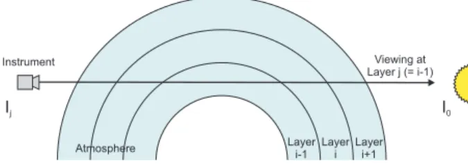
Fig. 1.The solar occultation viewing geometry.

The SCanning Imaging Absorption spectroMeter for Atmospheric CHartographY (SCIAMACHY; Bovensmann et al., 1999) is – as MIPAS and GOMOS – part of the payload of the European Environmental Satellite ENVISAT which was launched in 2002. SCIAMACHY performs spectral measurements in nadir, limb and lunar/solar occultation ge-ometry, covering almost continuously the wavelength range between about 220 and 2400 nm (Bovensmann et al., 1999). From these measurements column densities and profiles of various atmospheric constituents are derived (see e.g. Piters et al., 2006), among these also water vapour columns from nadir measurements (see e.g. No¨el et al., 2004, 2005). How-ever, up to now no water vapour profile data product from SCIAMACHY exists, although there are first successful at-tempts to derive such profiles from SCIAMACHY limb data. In this paper a new method to derive water vapour pro-files from SCIAMACHY solar occultation data is presented. Retrievals of atmospheric trace gas profiles from limb or oc-cultation measurements are often based on the optimal esti-mation (OE) method (see e.g. Rodgers, 1990). This method has proven to be appropriate for this purpose, as it in gen-eral produces reliable results which compare well with in-dependent data, see e.g. Rozanov et al. (2005, 2007), Palm et al. (2005), Meyer et al. (2005) or Amekudzi et al. (2005) for examples of (especially SCIAMACHY) retrievals using the OE method in different viewing geometries. The OE ap-proach usually involves an iterative process where radiative transfer calculations are required in each step. This makes OE methods relatively time consuming, which may become critical if large data sets – like those provided by satellites – need to be analysed. In many cases – like for limb appli-cations in the UV/Vis/NIR, where multiple scattering plays a large role – such an iterative radiative transfer scheme can not be avoided. Alternatively some retrieval methods (see e.g. K¨uhl et al., 2008) use a two-step approach which sepa-rates the derivation of slant column densities of the respec-tive absorber from the inversion. Another method used in the analysis of limb data is the Global Fit approach (Carlotti, 1988) in which a nonlinear least-squares fit is applied simul-taneously to the spectra for all tangent heights.

In solar occultation geometry, the measured quantity is not the scattered earthshine but the direct transmission of solar light. In this situation, the sun is directly in the field of view

(FOV) of the instrument and intensities are large. The con-tribution of light scattered from outside the FOV into the in-strument can be neglected. The accuracy of multiple scat-tering is therefore not as critical for retrievals from occul-tation measurements as for those from limb scattered radi-ation. However, radiative transfer calculations remain one limiting factor for the speed of the retrieval, especially in the case of so called line absorbers like water vapour, which re-quire high spectral resolution. Taking these considerations into account, the water vapour profile retrieval method de-scribed in this paper is based on an onion peeling approach (Russell and Drayson, 1972) to derive water vapour densi-ties starting from the upper atmospheric layers downwards. In each layer a method based on modified DOAS (Differ-ential Optical Absorption Spectroscopy) (Perner and Platt, 1979; Burrows et al., 1999; No¨el et al., 2004) is used to de-rive the corresponding water vapour density along the line of sight using a pre-calculated radiative transfer data base. In addition as DOAS strictly is applicable only in the optically thin case, a correction accounting for the non-linearity of the water vapour absorption (arising from non-resolved spectral lines) is applied.

The retrieval method is explained in more detail in the fol-lowing section. In Sect. 3 the application of the method to SCIAMACHY data is described. The results and a first vali-dation by comparison with independent data are then given in Sects. 4 and 5, followed by a discussion of errors in Sect. 6.

2 Retrieval method

2.1 General approach

The profile retrieval method is based on an onion peeling approach in which the atmosphere is divided into a number

Nlayerof horizontal layers. The retrieval starts at the top layer

and proceeds downwards, taking into account at each altitude the results of the upper layers. In solar occultation geometry the instrument is looking directly to the sun through the at-mosphere (see Fig. 1). The viewing geometry is therefore well defined. Because of the large intensities of the directly transmitted beam no multiple scattering processes need to be considered.

The basic premise is that – assuming a horizontally homo-geneous atmosphere – the absorption of light along a light path transecting the whole atmosphere may be written as the sum of the absorption of the individual altitude layers:

lnIj

I0

=Pj−

NXlayer

i=j

τij (1)

where all quantities are functions of wavelength. I0 is the

(3)

the optical depth of an absorber (i.e. water vapour) resulting from absorption in a layerifor an instrument looking at tan-gent altitudej. Ij is the corresponding measured spectrum

reaching the instrument under these viewing conditions, and

Ij/I0is the corresponding transmission. Note that because

only the directly transmitted light is taken into account, the signalIj is not affected by layers below the tangent height

j.Pj describes a low (in our case 2nd) order polynomial by

which all broadband spectral features (arising e.g. from Mie or Rayleigh scattering) are taken into account. This resem-bles the well-known Differential Optical Absorption Spec-troscopy (DOAS) approach (Perner and Platt, 1979) which is quite commonly used in the retrieval of nadir measurements (see e.g. Burrows et al., 1999). Therefore we call our method “Onion Peeling DOAS”.

The spectral range used in the retrieval is 928 nm to 968 nm. This wavelength range has been chosen, because there the water vapour absorption is on the one hand large enough for stratospheric retrievals and on the other hand saturation effects are not too strong. Between 928 nm and 968 nm mainly water vapour absorbs, but there is also a small absorption by ozone, which is also considered in the retrieval (see below).

2.2 Convolution effects

LetI_j0be the spectrum measured by an instrument looking at tangent heightj in the case that the atmosphere does not contain the absorber for which the partial optical depthsτij

are given. In this case, lnI

0 j

I0 =Pj, and Eq. (1) may be

re-written as: ln

I_j0 Ij

=

NXlayer

i=j

τij (2)

This equation only holds in the case that the spectral struc-tures are completely resolved by the measuring instrument. In general, the measured quantity is the atmospheric spec-trum convoluted by the insspec-trument spectral response func-tion, also called the instrument slit function. If we denote with hi this convolution, the left side of Eq. (2) becomes when using measured spectra:

lnhI

0

ji

hIji

(3) which is not identical to the convolution of Eq. (2):

lnhI

0

ji

hIji

6= hlnI

0

j

Ij

i = h

NXlayer

i=j

τiji =

NXlayer

i=j

hτiji (4)

To compensate for this, we define a “corrected” partial op-tical depthτ_ijc as:

τ_ijc := hτijicconv_j (5)

with

cconv_j := lnhI

0 ji

hIji

hlnI

0 j

Iji

(6)

which leads to the following modified version of Eq. (1) which is also fulfilled for convoluted spectra:

lnhIji hI0i

=Pj−

NXlayer

i=j

τ_ijc (7)

Note that Eqs. (1) and (7) are equivalent in the case that the atmospheric spectral structures are much broader than the strument slit function. However, since the SCIAMACHY in-strument does not resolve the individual water vapour lines this correction needs to be considered.

2.3 Density retrieval

In the optically thin case, the optical depthτij would be

pro-portional to the number densityni, i.e. the concentration of

the absorber in layeri, the absorption cross section and the length of the corresponding light path.

The relation between a modelled optical depthτ_ijrefand a real (measured) oneτijis therefore given by:

ai:=

ni

nref_i = τij

τ_ijref (8)

This leads to:

lnI

M

j

I₀M=Pj−

NXlayer

i=j

τ_ijrefai (9)

whereτ_ijref has to include the convolution correction factor

cconv_j andI_jMandI₀Mare the measured spectra at instrument spectral resolution.

Unfortunately, for water vapour in the spectral range con-sidered here the optically thin case can not be assumed. Fur-thermore, saturated and non-saturated water vapour absorp-tion lines are not resolved by the SCIAMACHY. As a conse-quence, the relation between optical depth and number den-sity becomes non-linear. This so-called saturation effect is taken into account by an additional correction factorciwhich

is a function of (only) density and altitude. ci is currently

considered as a scalar value. Taking into account the depen-dence of the other quantities from the wavelengthλleads to the following equation, assuming that only water vapour ab-sorbs in the spectral region under consideration:

ln

I_jM(λ)

I₀M(λ)=Pj(λ)−

NXlayer

i=j

τ_ijref(λ) ci(ni) ai (10)

Although water vapour absorption is dominant in the wave-length range used here (928–968 nm), ozone (O3) is

(4)

fit residuals, we also consider ozone as an absorber. There-fore, an additional sum of reference ozone optical depths

τO3,ref

ij , also derived from radiative transfer calculations and

then scaled by a factorbi, has to be taken into account. Note

that no additional correction factors are required for ozone because convolution and non-linearity effects do not play a role here and we are not interested in the absolute ozone amounts. This results in the following relation:

lnI

M

j (λ)

I₀M(λ)=Pj(λ)−

NXlayer

i=j

τ_ijref(λ)ci(ni)ai−

NXlayer

i=j

τO3,ref

ij (λ)bi (11)

For a given non-linearity correctionci the coefficients of

the polynomialPj and the scaling factorsai andbi (which

do not depend on wavelength) can be determined via a least squares fit using Eq. (11). Note thatci is a function ofni

and therefore alsoai. Consequently,ci needs to be adapted

in each iteration step of the fit. The retrieval starts at the top tangent height (j=Nlayer), which results in the

quanti-tiesPNlayer and the scaling factorsaNlayer andbNlayer. In the

retrieval for the next lowest tangent altitude (j=Nlayer−1)

the determined values for aNlayer and bNlayer are then used,

and so on, such that for each tangent heightj onlyaj and

bj (and the coefficients ofPj) need to be fitted. The water

vapour density at a certain altitudej is then given by:

nj=ajnrefj (12)

Obviously, one disadvantage of this method is that any errors of the higher tangent altitudes propagate downward. However, in the case of water vapour the coupling between the different layers is largely reduced by the exponential den-sity increase with decreasing altitude.

2.4 Determination of partial optical depths

The partial optical depths τ_ijref and τO3,ref

ij can be derived

from radiative transfer calculations. For this purpose, two transmission spectra need to be determined for an instrument looking at altitudej:

1. A spectrum Iij assuming an atmosphere where only

layericontains the absorber.

2. A spectrumI_j0assuming an atmosphere where the ab-sorber is not present at all.

The partial optical depth is then given by:

τij=ln

I_j0 Iij

(13) For the computation of the convolution correction according to Eq. (6) additionally the end-to-end spectraIj andI0are

required. All spectra have been derived using the radiative transfer model SCIATRAN (Rozanov et al., 2002), Version 2.2 in transmission mode. The involved water vapour cross

sections are taken from the HITRAN 2008 data base (Roth-man et al., 2009). The assumed reference atmosphere con-tains pressure, temperature and water vapour concentrations taken from model data provided by the European Centre for Medium Range Weather Forecasts (ECMWF) for a latitude of 67.5◦N and a longitude of 30◦W on 10 November 2005, 18:00 UT. This time and place corresponds to one of the col-locations between SCIAMACHY and ACE-FTS (see below), but this is actually an arbitrary choice.

Because the retrieval uses a fixed set of reference optical depths and saturation correction factors, the retrieval results are somewhat sensitive to the choice of the reference atmo-sphere. This is mainly because the water vapour absorption cross section is a function of temperature and (to a lesser degree) pressure. Depending on the actual atmospheric con-ditions which usually differ from the model assumptions this may cause systematic deviations in the retrieved profiles. Re-trieval studies with different model atmospheres have shown that this systematic effect is largest at lower altitudes where the deviations between the retrieved profiles may reach about 20% in extreme cases (e.g. when using a tropical atmosphere for a retrieval at higher latitudes). At altitudes above about 35 km there is almost no dependency on the reference atmo-sphere. The ECMWF model atmosphere used in this study is considered to be appropriate for the latitudinal range of the measurements (about 50–70◦N, see below), therefore no major systematic error contributions are expected from using a fixed background atmosphere.

The altitude grid for the radiative transfer calculations con-sists of 1 km intervals from 0 to to 50 km which is the max-imum altitude for the retrieval. The reference atmosphere, however, continues further upwards, therefore the topmost model altitude level has no upper limit but contains every-thing above. Currently, the retrieval is limited to altitudes above 15 km because below this height (and especially in the troposphere) densities and related non-linear effects in the optical depths become too large and also refraction be-comes more important such that the model assumptions are no longer valid.

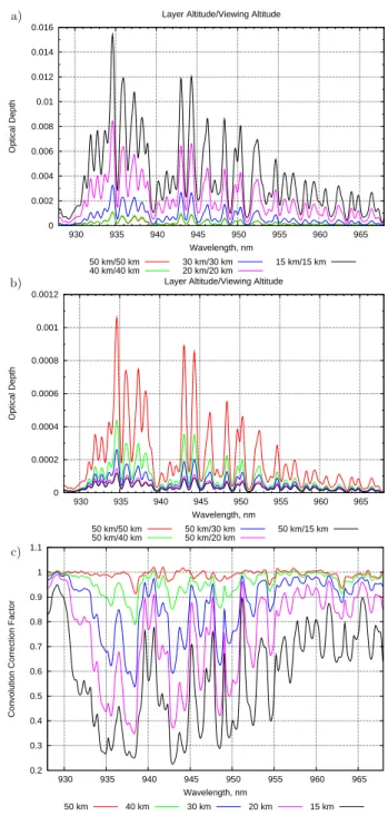
Figure 2 shows some examples for modelled partial op-tical depthsτ_ijrefof water vapour for different combinations of water vapour layer altitude indexi and viewing altitude indexj. In the case where the viewing altitude equals the layer which contains water vapour (Fig. 2a) the optical depth increases with decreasing altitude, as can be expected from the increasing water vapour concentration. For a fixed layer altitude (in Fig. 2b 50 km) the optical depths decrease with decreasing viewing altitude because the absorber concentra-tion along the light path decreases.

(5)

2.5 Determination of saturation correction

The saturation (or non-linearity) correction factorci(ni)is

also determined from radiative transfer calculations using the relation

lnhI

0

ji

hIji

=

NXlayer

i=j

τ_ijrefai ci (14)

which can be derived from Eq. (10) when taking modelled spectra instead of measured ones. Defining

τj:=ln

hI_j0i hIji

(15) and denoting withxthe spectral average over the fitting win-dow for quantityx, the following relation for the saturation correction can be derived:

cj=

τj−P

Nlayer

i=j+1τ ref

ij aici

aj τ_jjref

(16)

Using Eq. (16), starting from the top altitude (Nlayer) and

then propagating downwards each saturation correction fac-tor for a certain tangent altitude can be derived. Note that

τj is also a function of density, or the related scaling factors

ai. The density dependence ofcis derived by performing

ra-diative transfer calculations for water vapour profiles which are scaled by a height independent factor. The resulting den-sity dependence ofcis in fact an approximation, because – as can be seen from Eq. (16) – thecj depend not only on

the density in layerj (i.e.aj) but also on all densities (orai)

above. Therefore, different shapes of profiles will result in a different density dependence ofc. However, specifically for stratospheric water vapour this effect is considered to be small because of the exponential decrease of density with al-titude which limits the impact of alal-titudes which are much higher than the tangent altitude.

This way, a data base of saturation correction factorsci(ai)

is calculated for a set of scaling factors between 10% and 300%. In the retrieval, the required saturation correction fac-tors are then derived by interpolation.

Figure 3a shows the derived saturation correction factorc

as function of the used water vapour profile scaling factor for different tangent altitudes. In general, a smaller scaling fac-tor (i.e. lower water vapour densities thannref) results in a largercand vice versa. This is becauseci is multiplied to the

density scale factor in the retrieval formula (Eq. 11). For the reference atmosphere, the scaling factor and thus allai are

equal to 1, yielding that also allci are equal 1 (as it should

be). For a tangent altitude of 50 km the saturation correc-tion factor is close to 1 and does not depend much on the water vapour density. For lower tangent altitudes the satura-tion effect and also the density dependence becomes larger, although there is not much difference between the saturation correction factors for the lowest altitudes (15 km and 20 km).

a)

0 0.002 0.004 0.006 0.008 0.01 0.012 0.014 0.016

930 935 940 945 950 955 960 965

Optical Depth

Wavelength, nm Layer Altitude/Viewing Altitude

50 km/50 km 40 km/40 km

30 km/30 km 20 km/20 km

15 km/15 km

b)

0 0.0002 0.0004 0.0006 0.0008 0.001 0.0012

930 935 940 945 950 955 960 965

Optical Depth

Wavelength, nm Layer Altitude/Viewing Altitude

50 km/50 km 50 km/40 km

50 km/30 km 50 km/20 km

50 km/15 km

c)

0.2 0.3 0.4 0.5 0.6 0.7 0.8 0.9 1 1.1

930 935 940 945 950 955 960 965

Convolution Correction Factor

Wavelength, nm

50 km 40 km 30 km 20 km 15 km

Fig. 2.Modelled partial optical depths (including convolution cor-rection). The “layer altitude” is the only altitude containing water vapour. The “viewing altitude” corresponds to the observed tan-gent altitude. (a)Layer altitude equals viewing altitude. (b)Same layer altitude (50 km) but different viewing altitudes. (c) Convolu-tion correcConvolu-tion factor as funcConvolu-tion of wavelength for different tangent altitudes.

(6)

a)

0.6 0.8 1 1.2 1.4 1.6 1.8

0 50 100 150 200 250 300

Saturation Correction Factor

Water Vapour Profile Scaling Factor, %

15 km 20 km 30 km 40 km 50 km

b)

15 20 25 30 35 40 45 50

0.9 0.92 0.94 0.96 0.98 1 1.02 1.04 1.06 1.08 1.1

Altitude, km

Density Ratio Retrieved/True

70%

80% 100% 90% 110%120% 130%

Fig. 3.Results for simulated data.(a)Saturation correction factors as function of the water vapour scaling factor for different tangent altitudes. (b)Results of a retrieval on simulated data using scaled water vapour profiles. The different curves correspond to different scaling factors.

2.6 Consistency check

A consistency check of the retrieval method is performed by application of Eq. (11) to simulated data, equivalent to those data from which the saturation correction factors are com-puted. The input water vapour profiles have been scaled by factors between 70% and 130%, thus covering at least the expected variability of stratospheric water vapour which is in the order of 20%. No additional noise has been added to the simulated data. The resulting ratios of the retrieved water vapour density profiles to the true one are plotted in Fig. 3b as function of altitude.

For a self-consistent retrieval the density ratio should be equal to 1 for all altitudes. As can be seen from Fig. 3b this is only the case for the reference density (100% scaling). For scaling factors different from 1 there are deviations of up to ±10%, increasing with the scale factor and with a maximum between 20 and 25 km. The main reason for these differ-ences is that the retrieval uses a scalar saturation correction

factor instead of a spectrally resolved one. Because of this, the accuracy of the retrieval method described here is cur-rently limited by the saturation correction to about 10%.

Especially above about 30 km small oscillations in the re-trieved ratios occur. This kind of oscillations is well known from limb or occultation profile retrievals (see e.g. v. Clar-mann et al., 1991; Sofieva et al., 2004). One possibility to overcome this problem is to add constraints on the smooth-ness of the profile to the retrieval as a priori information. The retrieval method used in the present paper does not contain such smoothness constraints. Instead, the profiles resulting from SCIAMACHY measurements are smoothed after the retrieval considering the vertical resolution of the instrument. This is described in the next section.

3 Application to SCIAMACHY

The SCIAMACHY instrument performs solar occultation measurements usually once per orbit during sunrise1_{. With}

an orbital period of about 100 min this results in 14 to 15 oc-cultation measurements per day. SCIAMACHY comprises eight channels of 1024 pixels each, covering almost continu-ously the spectral range between about 220 nm and 2400 nm. In the spectral range of the water vapour retrieval (928 to 968 nm) the spectral resolution is about 0.52 nm. The SCIA-MACHY instantaneous field of view (IFOV) in solar occulta-tion mode is about 0.72◦×0.045◦; this corresponds to a ver-tical resolution at the tangent point of about 2.6 km. The hor-izontal resolution (across track) at the tangent point is about 30 km, limited by the size of the sun (about 0.5◦).

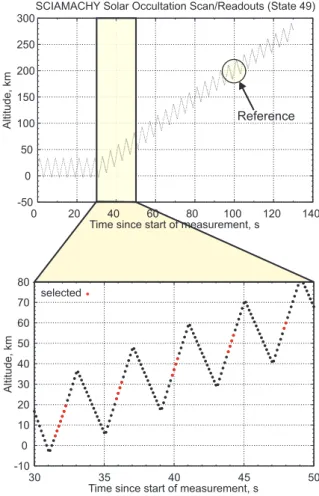
A solar occultation measurement is performed by SCIA-MACHY in the following way: Before sunrise there are for 30 s vertical scans of ±0.33◦ around an altitude of about 17 km. As soon as the centre of the sun reaches this alti-tude, the rising sun is followed upwards while continuing the upward/downward scans. Above 100 km there are dif-ferent modes of solar occultation measurements performed; for the water vapour profile retrieval we use only those mea-surements where the vertical scan over the sun is continued up to almost 300 km.

For the spectral range considered here there are 16 read-outs per vertical scan (either downward or upward). For the retrieval a subset of these measurements is used; namely only those data when the sun is already rising but below 60 km. Furthermore, only data from the central part of the upward scans are used. This results in about 20 spectra at differ-ent tangdiffer-ent altitudes between 0 and 60 km. However, as ex-plained in the previous section, retrieval results below 15 km are currently not used. This is illustrated in Fig. 4 for a typ-ical SCIAMACHY solar occultation measurement. In addi-tion, corresponding measurements at about 200 km altitude

1_{Note that although the SCIAMACHY instrument sees a rising}

(7)

are used as reference spectrum (I0) by which the lower

alti-tude spectra are divided; care is taken that only spectra of the same relative position on the sun (i.e. matching readouts in the vertical scan) are combined. This is necessary because of the different filling of the IFOV.

It is a prerequisite of the retrieval method used here that the modelled optical depths and the measured spectra are on the same altitude grid. To avoid a re-calculation of optical depths for each individual measurement the (logarithms of the) mea-sured SCIAMACHY spectra are linearly interpolated to the retrieval altitude grid before the retrieval. After the retrieval, the derived profiles are smoothed by application of a box-car filter of width 2.6 km, which is the vertical size of the SCIAMACHY instantaneous field of view. This smoothing is done to avoid retrieval artefacts resulting from (1) insta-bilities/oscillations in the retrieved profiles due to a lack of information, (2) the interpolation of the measured transmis-sions to the (finer) retrieval altitude grid, and (3) the coarser vertical resolution of the SCIAMACHY measurements com-pared to the retrieval grid spacing of 1 km.

4 Results

Figure 5 shows an example for retrieval results for a SCIAMACHY measurement in orbit 19 333 on 10 Novem-ber 2005. Panel a depicts the measured signal (lnI /I0) at

50 km together with the fitted spectrum and the resulting rel-ative residual. The signal at this altitude is low and noisy, and the residual is quite large, but nevertheless the fit is success-ful. Panel b shows the same for a tangent altitude of 20 km. Here, the densities are much higher and also the absorption structures are much better pronounced. Consequently, the relative fit residuals are much smaller. However, a closer look at the residuals reveals larger differences between fit and measurements at spectral regions where absorption is higher (e.g. around 935 nm). This is an indication that saturation is not completely corrected, most likely because the currently implemented saturation correction does not depend on wave-length. Here, there is room for improvement of the retrieval method.

Figure 5c shows the retrieved profile of water vapour. The un-smoothed data are depicted by the blue line, the smoothed data by the red line. Below about 30 km there is almost no difference between the smoothed and un-smoothed pro-file. The green circles indicate the original measurement tangent heights. The error bars give the estimated retrieval error derived from the fit, which (in the logarithmic plot) increases with height and is considerably high (about 50%) above 45 km.

Up to now, all SCIAMACHY data from August 2002 until October 2009 have been processed using the Onion Peeling DOAS method. The resulting profiles are shown in Fig. 6a. For this plot all data of one day (up to 13 profiles at different longitudes but almost the same latitude) have been averaged.

-50 0 50 100 150 200 250 300

0 20 40 60 80 100 120 140

Altitude,km

Time since start of measurement, s

SCIAMACHY Solar Occultation Scan/Readouts (State 49)

Altitude,km

Time since start of measurement, s -10

0 10 20 30 40 50 60 70 80

35 40 45 50

30 selected

Reference

Fig. 4. Tangent altitudes of channel 5 readouts during a typical SCIAMACHY solar occultation measurement. Only those altitudes marked by red points are used in the retrieval. Reference spectra (I0) are taken from the upward scan around 100 s after the start of

the measurement in about 200 km altitude.

The latitudinal distribution of the data is shown in the top of the figure. As can be seen from this, SCIAMACHY occul-tation measurements are restricted to northern mid-latitudes between about 50◦ _{and 70}◦_{. Because of the sun-fixed} EN-VISAT orbit the latitudinal variation is the same for each year. The black curve in the lower part of the figure shows the average tropopause height (defined as temperature min-imum), which has been derived from collocated ECMWF temperature profiles provided every 6 h on a 1.5◦×1.5◦ lati-tude/longitude grid.

(8)

a)

-0.0042 -0.004 -0.0038 -0.0036 -0.0034 -0.0032 -0.003 -0.0028 -0.0026 -0.0024

925 930 935 940 945 950 955 960 965 970

ln(I/I

0

)

SCIAMACHY Occultation H₂O Retrieval (orbit 19333)

50 km

Signal Fit

-0.2 -0.15 -0.1 -0.05 0 0.05 0.1 0.15 0.2 0.25 0.3

925 930 935 940 945 950 955 960 965 970

Residual, (Fit-Signal)/Signal

Wavelength, nm

b)

-0.23 -0.22 -0.21 -0.2 -0.19 -0.18 -0.17 -0.16 -0.15

925 930 935 940 945 950 955 960 965 970

ln(I/I

0

)

SCIAMACHY Occultation H₂O Retrieval (orbit 19333)

20 km Signal

Fit

-0.03 -0.02 -0.01 0 0.01 0.02 0.03

925 930 935 940 945 950 955 960 965 970

Residual, (Fit-Signal)/Signal

Wavelength, nm c)

15 20 25 30 35 40 45 50

1e+10 1e+11 1e+12 1e+13 1e+14

Altitude, km

H₂O Density, molecules/cm3 SCIAMACHY Occultation 20051110 Orbit 19333

SCIAMACHY (smoothed) SCIAMACHY (on retrieval grid) SCIAMACHY (on meas. grid)

Fig. 5. Example fit results for a SCIAMACHY occultation mea-surement on 10 November 2005. (a)Measured signal and fit (top) and corresponding residual (bottom) for 50 km tangent altitude. (b)Same for 20 km tangent altitude. (c)Resulting water vapour profile from SCIAMACHY data (smoothed, un-smoothed, and in-terpolated to measurement altitude grid).

a)

40 50 60 70

Lat (deg)

01-Jan-03 01-Jan-04 01-Jan-05 01-Jan-06 01-Jan-07 01-Jan-08 01-Jan-09 10

20 30 40 50

Avg. Tropopause 01-Jan-03 01-Jan-04 01-Jan-05 01-Jan-06 01-Jan-07 01-Jan-08 01-Jan-09

10 20 30 40 50

Altitude (km)

1011 1012 1013 1014

Water Vapour Density (molecules/cm3₎

b)

40 50 60 70

Lat (deg)

01-Jan-03 01-Jan-04 01-Jan-05 01-Jan-06 01-Jan-07 01-Jan-08 01-Jan-09 10

20 30 40 50

Avg. Tropopause 01-Jan-03 01-Jan-04 01-Jan-05 01-Jan-06 01-Jan-07 01-Jan-08 01-Jan-09

10 20 30 40 50

Altitude (km)

3 4 5 6 7 8 9

Water Vapour VMR (ppmv)

Fig. 6. Daily averaged water vapour profiles derived from SCIA-MACHY occultation measurements with the Onion Peeling DOAS method. (a)Number density profiles. The latitudinal range of the SCIAMACHY measurements is indicated on top of the figures. The black curve shows the average tropopause height, derived from col-located ECMWF data. Periods of reduced SCIAMACHY data qual-ity (due to instrument switch-offs or decontamination periods) have been masked out (vertical grey bars). (b)Same plot for volume mixing ratio (VMR) profiles.

(9)

5 Validation

For a first validation, the derived SCIAMACHY water vapour profiles have been compared with collocated wa-ter vapour profiles from the European Centre for Medium Range Weather Forecasts (ECMWF) and from the Atmo-spheric Chemistry Experiment Fourier Transform Spectrom-eter (ACE-FTS).

The ECMWF water vapour density profile has been de-rived from analysed meteorological profiles of pressure, tem-perature and specific humidity, which are provided every 6 h on a 1.5◦×1.5◦latitude/longitude grid. The ECMWF profile closest in time and space has been selected.

The ACE-FTS instrument is the primary payload of the Canadian SCISAT-1 satellite which was launched in Au-gust 2003 (Bernath et al., 2005). ACE-FTS performs so-lar occultation measurements in the infrared spectral range (2.2 to 13.3 µm) and provides altitude profiles for tempera-ture, pressure and the volume mixing ratios (VMRs) of sev-eral atmospheric molecules – including water vapour – be-tween typically 10 and 100 km. The second instrument on SCISAT-1, ACE-MAESTRO (Measurement of Aerosol Ex-tinction in the Stratosphere and Troposphere Retrieved by Occultation) is a UV-Vis spectrometer which also provides – among other products – water vapour profiles. However, in the present paper we only compare with ACE-FTS pro-files (Version 2.2). The ACE water vapour propro-files have been validated by comparisons with results from several space-borne, balloon-borne and ground-based sensors (Car-leer et al., 2008), resulting in an agreement within about 5–10% in the stratosphere (15 to 70 km). For the compari-son with SCIAMACHY data the VMRs have been converted to number densities using temperature and pressure profiles also provided by FTS. The criteria for collocated ACE-FTS and SCIAMACHY data sets are that the data have to be obtained on the same day within a maximum tangent point distance of 500 km. For the comparison all data have been interpolated to the SCIAMACHY retrieval altitude grid.

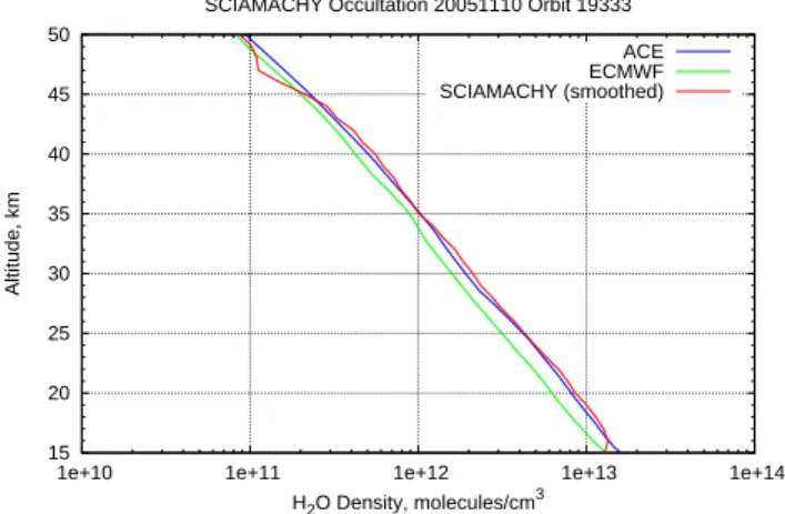
Figure 7 shows the (smoothed) SCIAMACHY water vapour profile from Fig. 5c in comparison with ECMWF and ACE-FTS data. In this case, the selected ACE-FTS profile is obtained at the same day as the SCIAMACHY data at almost the same location (distance only about 16 km). The shown ECMWF profile is in fact the one which was used in the ra-diative transfer calculations to derive partial optical depths and saturation correction factors (see Sect. 2).

Whereas the ECMWF water vapour densities are system-atically lower than both satellite data, there is a quite good agreement between the ACE-FTS and SCIAMACHY results. This is confirmed by a more extended analysis involving 408 collocations between SCIAMACHY and ACE-FTS and the corresponding ECMWF data in the years 2004 to 2007. The results of the inter-comparisons are shown in Fig. 8.

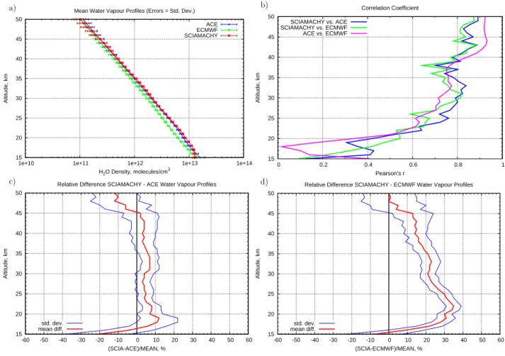
Figure 8a shows the average water vapour profiles of SCIAMACHY, FTS and ECMWF. Whereas the

15 20 25 30 35 40 45 50

1e+10 1e+11 1e+12 1e+13 1e+14

Altitude, km

H2O Density, molecules/cm3

SCIAMACHY Occultation 20051110 Orbit 19333

ACE ECMWF SCIAMACHY (smoothed)

Fig. 7. SCIAMACHY water vapour profile on 10 Novem-ber 2005. Comparison of SCIAMACHY water vapour profile from 10 November 2005 with matching ACE and ECMWF profiles.

FTS and SCIAMACHY data agree quite well over almost the whole altitude range, the mean ECMWF water vapour concentrations are systematically lower than both ACE-FTS and SCIAMACHY results at all altitudes. The error bars in Fig. 8a comprise the standard deviation of the profiles at each altitude and do not consider errors of the retrieved wa-ter vapour data. The errors bars therefore are an indicator for the variability in water vapour seen by the instruments and the model. For all data sets the variability is lowest between 20 and 25 km and increases at higher altitudes and towards the troposphere.

In panel b of Fig. 8 the correlation between the data sets (SCIAMACHY vs. ACE-FTS, SCIAMACHY vs. ECMWF and ACE-FTS vs. ECMWF) is shown as a function of alti-tude. The correlation describes how well variations in water vapour profiles by ACE-FTS or ECMWF are reproduced by the SCIAMACHY data, which is an important information to e.g. assess the potential to derive stratospheric water vapour trends. The observed correlation is very similar for all three combinations and considerably high at altitudes above 30 km (Pearson’s r varies around 0.7–0.9 there), but significantly drops down for lower altitudes. Above about 20 km these low correlations are possibly related to the smaller water vapour variations at these altitudes, as can be seen from the stan-dard deviations in panel a. Below 20 km variations become higher; there, atmospheric effects like refraction (which is not considered in the SCIAMACHY retrieval) may play a role. This has to be investigated further.

(10)

a)

15 20 25 30 35 40 45 50

1e+10 1e+11 1e+12 1e+13 1e+14

Altitude, km

H₂O Density, molecules/cm3

Mean Water Vapour Profiles (Errors = Std. Dev.)

ACE ECMWF SCIAMACHY

b)

15 20 25 30 35 40 45 50

0 0.2 0.4 0.6 0.8 1

Altitude, km

Pearson’s r Correlation Coefficient

SCIAMACHY vs. ACE SCIAMACHY vs. ECMWF ACE vs. ECMWF

c)

15 20 25 30 35 40 45 50

-60 -50 -40 -30 -20 -10 0 10 20 30 40 50 60

Altitude, km

(SCIA-ACE)/MEAN, %

Relative Difference SCIAMACHY - ACE Water Vapour Profiles

std. dev. mean diff.

d)

15 20 25 30 35 40 45 50

-60 -50 -40 -30 -20 -10 0 10 20 30 40 50 60

Altitude, km

(SCIA-ECMWF)/MEAN, %

Relative Difference SCIAMACHY - ECMWF Water Vapour Profiles

std. dev. mean diff.

Fig. 8.Results of comparison between 408 collocated SCIAMACHY, ACE-FTS and ECMWF water vapour profiles.(a)Mean profiles; the error bars denote the standard deviation of the profiles.(b)Correlation between profiles as function of altitude.(c)Mean relative deviation between SCIAMACHY and ACE-FTS profiles and corresponding standard deviation.(d)As (c), but for comparison with ECMWF data.

As can be seen from Fig. 8c, the SCIAMACHY wa-ter vapour concentrations are systematically higher than the ACE-FTS values by about 5% between 20 and 45 km. Below and above this altitude range deviations are somewhat larger. As noted before, the results above 45 km are associated with a significant retrieval error and therefore less reliable. Be-low about 18 km the SCIAMACHY water vapour densities decrease significantly as can also be seen in subpanel a. This is considered to be related to tropospheric effects which limit the applicability of the SCIAMACHY retrieval at lower al-titudes. The standard deviation of the differences is only about 5% except for the lowest and highest altitudes where it reaches about 10–15%

The comparison with ECWMF data (Fig. 8d) confirms a systematic positive offset between SCIAMACHY and ECMWF water vapour profiles of about 15 to 35%, largest between 20 and 25 km. The standard deviation is except for the highest altitudes again small (5–10%).

6 Discussion of errors

To judge upon the quality of the SCIAMACHY water vapour density data various error sources of the retrieval (most of them mentioned before) are summarised and discussed in this section.

The precision of the derived water vapour densities esti-mated from the residuals of the retrieval (when applied to real measurement data) is typically in the order of 10–20% below 45 km (see Fig. 5 for an example) and usually below 15% between 20 and 40 km. This includes random error components resulting from instrumental noise.

(11)

However, systematic offsets are expected due to insuffi-ciencies of the (scalar) saturation correction (see Fig. 3). The actual error which results from this depends on how large the ‘true’ atmospheric conditions differ from the ones assumed in the radiative transfer calculations. Taking into account typical variabilities of water vapour as shown in Fig. 6 the maximum error due to limited saturation correction is esti-mated to be about 10% at around 25 km. This error is cur-rently considered to be the major source of uncertainties for the water vapour product. Because the chosen atmospheric conditions in the radiative transfer are based on ECMWF data, they are considered to be quite representative such that the specific choice of the reference profiles should (on aver-age) have only a minor impact on the retrieval results.

Another potential systematic error, not mentioned before, arises from the SCIAMACHY pointing knowledge, i.e. the accuracy of the tangent heights. Currently, SCIAMACHY tangent heights are expected to be accurate within some 100 m (with some seasonal effects), which translates into an error of water vapour densities in the order of 1–3%.

Other potential systematic error sources are the selected slit function and the knowledge of the line parameters given in the HITRAN (Rothman et al., 2009) data base used in the radiative transfer calculations. These errors are difficult to quantify, but since the most actual data have been used in the retrieval this error is considered to be small.

Based on the values given above, the overall uncertainty of the SCIAMACHY water vapour densities for a single mea-surement is expected to be in the order of 10–15%.

The accuracy of the water vapour product can only be as-sessed after validation. Based on the comparison with ACE-FTS data shown in Sect. 5 an accuracy of the SCIAMACHY water vapour profiles of about 5% (mean deviation, with a standard deviation of also about 5%) in the altitude range 20 to 45 km is estimated.

7 Conclusions

The new “Onion Peeling DOAS” retrieval method to derive water vapour density profiles from SCIAMACHY solar oc-cultation measurements in the spectral region 928–968 nm has shown to provide reasonable results in the altitude region 15–45 km. The estimated precision of the SCIAMACHY wa-ter vapour profiles is 10 to 20% in this altitude range and typically better than 15% between 20 and 40 km. ECMWF water vapour densities are generally lower than both ACE-FTS and SCIAMACHY data at all heights. The maximum deviation between SCIAMACHY and ECMWF results is about 35% between 20 and 25 km. Comparisons with ACE-FTS show a quite good agreement at altitudes between 20 and 45 km where mean relative deviations are below about 5%, with SCIAMACHY results being typically larger than those of ACE-FTS. Based on this, an accuracy of the SCIA-MACHY product of about 5% (±5%) is estimated. This is

within the estimated systematic errors of the SCIAMACHY retrieval which are in the order of 10–15%, mainly limited by the handling of saturation effects. For comparison, ACE validation results (Carleer et al., 2008) show an agreement of ACE-FTS water vapour profiles with other data sets in the stratosphere (15 to 70 km) of about 5–10%, which is in line with the SCIAMACHY data. Especially at higher alti-tudes there is a good correlation between the ACE-FTS and SCIAMACHY profiles, indicating that both instruments are capable to identify similar changes in water vapour concen-trations. Taking into account the simplicity of the SCIA-MACHY retrieval method, which (intentionally) only uses a very limited radiative transfer data base, these results are very promising.

In principle, the Onion Peeling DOAS method is not re-stricted to the application to water vapour. It may also be used for the retrieval of other trace gases (like ozone) where saturation is less critical. This will be investigated in the fu-ture.

Acknowledgements. SCIAMACHY is a national contribution to

the ESA ENVISAT project, funded by Germany, The Netherlands, and Belgium. SCIAMACHY data have been provided by ESA. The Atmospheric Chemistry Experiment (ACE), also known as SCISAT, is a Canadian-led mission mainly supported by the Canadian Space Agency and the Natural Sciences and Engineering Research Council of Canada. We thank the European Center for Medium Range Weather Forecasts (ECMWF) for providing us with analysed meteorological fields. This work has been funded by DLR Space Agency (Germany), grant 50EE0727, and by the University of Bremen.

Edited by: R. Sussmann

References

Amekudzi, L., Bracher, A., Meyer, J., Rozanov, A., Bovensmann, H., and Burrows, J.: Lunar occultation with SCIAMACHY: First retrieval results, Adv. Space Res., 36, 906–914, doi:10.1016/j. asr.2005.03.017, 2005.

Aumann, H. H., Chahine, M. T., Gautier, C., Goldberg, M. D., Kalnay, E., McMillin, L. M., Revercomb, H., Rosenkranz, P. W., Smith, W. L., Staelin, D. H., Strow, L. L., and Susskind, J.: AIRS/AMSU/HSB on the Aqua Mission: De-sign, Science Objectives, Data Products, and Processing Systems, IEEE Trans. Geosc. Rem. Sens., 41, 253–264, doi:10.1109/TGRS.2002.808356, 2003.

Barnes, J. E., Kaplan, T., V¨omel, H., and Read, W. G.: NASA/Aura/Microwave Limb Sounder water vapor validation at Mauna Loa Observatory by Raman lidar, J. Geophys. Res., 113, D15S03, doi:10.1029/2007JD008842, 2008.

(12)

Rochon, Y. J., Rowlands, N., Semeniuk, K., Simon, P., Skel-ton, R., Sloan, J. J., Soucy, M.-A., Strong, K., Tremblay, P., Turnbull, D., Walker, K. A., Walkty, I., Wardle, D. A., Wehrle, V., Zander, R., and Zou, J.: Atmospheric Chemistry Experiment (ACE): Mission overview, Geophys. Res. Lett., 32, L15S01, doi: 10.1029/2005GL022386, 2005.

Bovensmann, H., Burrows, J. P., Buchwitz, M., Frerick, J., No¨el, S., Rozanov, V. V., Chance, K. V., and Goede, A. H. P.: SCIA-MACHY – Mission Objectives and Measurement Modes, J. At-mos. Sci., 56, 127–150, 1999.

Burrows, J. P., Weber, M., Buchwitz, M., Rozanov, V., Ladst¨atter-Weißenmayer, A., Richter, A., de Beek, R., Hoogen, R., Bram-stedt, K., Eichmann, K.-U., Eisinger, M., and Perner, D.: The Global Ozone Monitoring Experiment (GOME): Mission Con-cept and First Scientific Results, J. Atmos. Sci., 56, 151–175, 1999.

Carleer, M. R., Boone, C. D., Walker, K. A., Bernath, P. F., Strong, K., Sica, R. J., Randall, C. E., V¨omel, H., Kar, J., H¨opfner, M., Milz, M., von Clarmann, T., Kivi, R., Valverde-Canossa, J., Sioris, C. E., Izawa, M. R. M., Dupuy, E., McElroy, C. T., Drummond, J. R., Nowlan, C. R., Zou, J., Nichitiu, F., Lossow, S., Urban, J., Murtagh, D., and Dufour, D. G.: Validation of wa-ter vapour profiles from the Atmospheric Chemistry Experiment (ACE), Atmos. Chem. Phys. Discuss., 8, 4499–4559, 2008, http://www.atmos-chem-phys-discuss.net/8/4499/2008/. Carlotti, M.: Global-fit approach to the analysis of limb-scanning

atmospheric measurements, Appl. Opt., 27, 3250–3254, doi:10. 1364/AO.27.003250, 1988.

Dhomse, S., Weber, M., and Burrows, J.: The relationship between tropospheric wave forcing and tropical lower stratospheric water vapor, Atmos. Chem. Phys., 8, 471–480, 2008,

http://www.atmos-chem-phys.net/8/471/2008/.

Fischer, H., Birk, M., Blom, C., Carli, B., Carlotti, M., von Clar-mann, T., Delbouille, L., Dudhia, A., Ehhalt, D., EndeClar-mann, M., Flaud, J. M., Gessner, R., Kleinert, A., Koopman, R., Langen, J., L´opez-Puertas, M., Mosner, P., Nett, H., Oelhaf, H., Perron, G., Remedios, J., Ridolfi, M., Stiller, G., and Zander, R.: MIPAS: an instrument for atmospheric and climate research, Atmos. Chem. Phys., 8, 2151–2188, 2008,

Hagan, D. E., Webster, C. R., Farmer, C. B., May, R. D., Her-man, R. L., Weinstock, E. M., Christensen, L. E., Lait, L. R., and Newman, P. A.: Validating AIRS upper atmosphere water vapor retrievals using aircraft and balloon in situ measurements, Geophys. Res. Lett., 31, L21103, doi:10.1029/2004GL020302, 2004.

K¨uhl, S., Pukite, J., Deutschmann, T., Platt, U., and Wagner, T.: SCIAMACHY limb measurements of NO2, BrO and OClO.

Re-trieval of vertical profiles: Algorithm, first results, sensitivity and comparison studies, Adv. Space Res., 42, 1747–1764, doi: 10.1016/j.asr.2007.10.022, 2008.

Kyrölä, E., Tamminen, J., Leppelmeier, G. W., Sofieva, V., Has-sinen, S., Bertaux, J. L., Hauchecorne, A., Dalaudier, F., Cot, C., Korablev, O., Fanton d’Andon, O., Barrot, G., Mangin, A., Théodore, B., Guirlet, M., Etanchaud, F., Snoeij, P., Koopman, R., Saavedra, L., Fraisse, R., Fussen, D., and Vanhellemont, F.: GOMOS on Envisat: an overview, Adv. Space Res., 33, 1020– 1028, 2004.

Meyer, J., Bracher, A., Rozanov, A., Schlesier, A. C., Bovensmann,

H., and Burrows, J. P.: Solar occultation with SCIAMACHY: algorithm description and first validation, Atmos. Chem. Phys., 5, 1589–1604, 2005,

Milz, M., Clarmann, T. v., Bernath, P., Boone, C., Buehler, S. A., Chauhan, S., Deuber, B., Feist, D. G., Funke, B., Glatthor, N., Grabowski, U., Griesfeller, A., Haefele, A., Höpfner, M., Kämpfer, N., Kellmann, S., Linden, A., Müller, S., Nakajima, H., Oelhaf, H., Remsberg, E., Rohs, S., Russell III, J. M., Schiller, C., Stiller, G. P., Sugita, T., Tanaka, T., Vömel, H., Walker, K., Wetzel, G., Yokota, T., Yushkov, V., and Zhang, G.: Validation of water vapour profiles (version 13) retrieved by the IMK/IAA scientific retrieval processor based on full resolution spectra mea-sured by MIPAS on board Envisat, Atmos. Meas. Tech., 2, 379– 399, 2009,

http://www.atmos-meas-tech.net/2/379/2009/.

Murtagh, D., Frisk, U., Merino, F., Ridal, M., Jonsson, A., Stegman, J., Witt, G., Eriksson, P., Jiménez, C., Megie, G., de la Noë, J., Ricaud, P., Baron, P., Pardo, J. R., Hauchcorne, A., Llewellyn, E. J., Degenstein, D. A., Gattinger, R. L., Lloyd, N. D., Evans, W. F., McDade, I. C., Haley, C. S., Sioris, C., von Savigny, C., Solheim, B. H., McConnell, J. C., Strong, K., Richardson, E. H., Leppelmeier, G. W., Kyrölä, E., Auvinen, H., and Oikarinen, L.: An overview of the Odin atmospheric mission, Can. J. Phys., 80, 309–319, doi:10.1139/P01-157, 2002.

Nedoluha, G. E., Bevilacqua, R. M., Hoppel, K. W., Lumpe, J. D., and Smit, H.: Polar Ozone and Aerosol Measurement III mea-surements of water vapor in the upper troposphere and lower-most stratosphere, J. Geophys. Res., 107, 4103, doi:10.1029/ 2001JD000793, 2002.

No¨el, S., Buchwitz, M., and Burrows, J. P.: First retrieval of global water vapour column amounts from SCIAMACHY measure-ments, Atmos. Chem. Phys., 4, 111–125, 2004,

No¨el, S., Buchwitz, M., Bovensmann, H., and Burrows, J. P.: Val-idation of SCIAMACHY AMC-DOAS water vapour columns, Atmos. Chem. Phys., 5, 1835–1841, 2005,

Palm, M., v. Savigny, C., Warneke, T., Velazco, V., Notholt, J., K¨unzi, K., Burrows, J., and Schrems, O.: Intercomparison of O3profiles observed by SCIAMACHY and ground based

mi-crowave instruments, Atmos. Chem. Phys., 5, 2091–2098, 2005, http://www.atmos-chem-phys.net/5/2091/2005/.

Perner, D. and Platt, U.: Detection of Nitrous Acid in the Atmo-sphere by Differential Optical Absorption, Geophys. Res. Lett., 6, 917–920, 1979.

Piters, A. J. M., Bramstedt, K., Lambert, J.-C., and Kirchhoff, B.: Overview of SCIAMACHY validation: 2002–2004, Atmos. Chem. Phys., 6, 127–148, 2006,

Rodgers, C. D.: Characterization and Error Analysis of Profiles Re-trieved From Remote Sounding Measurements, J. Geophys. Res., 95, 5587–5595, 1990.

(13)

Nau-menko, O. V., Nikitin, A. V., Orphal, J., Perevalov, V. I., Perrin, A., Predoi-Cross, A., Rinsland, C., Rotger, M., Simeckov´a, M., Smith, M. A. H., Sung, K., Tashkun, S. A., Tennyson, J., Toth, R. A., Vandaele, A. C., and Auwera, J. V.: The HITRAN 2008 molecular spectroscopic database, J. Quant. Spectr. Rad. Transf., 110, 533–572, doi:10.1016/j.jqsrt.2009.02.013, 2009.

Rozanov, A., Bovensmann, H., Bracher, A., Hrechanyy, S., Rozanov, V., Sinnhuber, M., Stroh, F., and Burrows, J.: NO₂ and BrO vertical profile retrieval from SCIAMACHY limb mea-surements: Sensitivity studies, Adv. Space Res., 36, 846–854, doi:10.1016/j.asr.2005.03.013, 2005.

Rozanov, A., Eichmann, K.-U., von Savigny, C., Bovensmann, H., Burrows, J. P., von Bargen, A., Doicu, A., Hilgers, S., Godin-Beekmann, S., Leblanc, T., and McDermid, I. S.: Comparison of the inversion algorithms applied to the ozone vertical profile retrieval from SCIAMACHY limb measurements, Atmos. Chem. Phys., 7, 4763–4779, 2007,

Rozanov, V. V., Buchwitz, M., Eichmann, K.-U., de Beek, R., and Burrows, J. P.: SCIATRAN – a new radiative transfer model for geophysical applications in the 240–2400 nm spectral region: The pseudo-spherical version, Adv. Space Res., 29, 1831–1835, 2002.

Russell, III, J. M. and Drayson, S. R.: The Inference of Atmospheric Ozone Using Satellite Horizon Measurements in the 1042 cm−1 Band, J. Atmos. Sci., 29, 376–390, 1972.

Russell, III, J. M., Gordley, L. L., Park, J. H., Drayson, S. R., Hes-keth, W. D., Cicerone, R. J., Tuck, A. F., Frederick, J. E., Harries, J. E., and Crutzen, P. J.: The Halogen Occultation Experiment, J. Geophys. Res., 98, 10777–10797, 1993.

Sofieva, V. F., Tamminen, J., Haario, H., Kyr¨ol¨a, E., and Lehtinen, M.: Ozone profile smoothness as a priori information in the in-version of limb measurements, Ann. Geophys., 22, 3411–3420, 2004,

http://www.ann-geophys.net/22/3411/2004/.

Thomason, L. W., Burton, S. P., Iyer, N., Zawodny, J. M., and An-derson, J.: A revised water vapor product for the Stratospheric Aerosol and Gas Experiment (SAGE) II version 6.2 data set, J. Geophys. Res., 109, doi:10.1029/2003JD004465, 2004. Thomason, L. W., Poole, L. R., and Randall, C. E.: SAGE III

aerosol extinction validation in the Arctic winter: comparisons with SAGE II and POAM III, Atmos. Chem. Phys., 7, 1423– 1433, 2007,

Thornton, H. E., Jackson, D. R., Bekki, S., Bormann, N., Errera, Q., Geer, A. J., Lahoz, W. A., and Rharmili, S.: The ASSET intercomparison of stratosphere and lower mesosphere humidity analyses, Atmos. Chem. Phys., 9, 995–1016, 2009,

Urban, J., Lautié, N., Murtagh, D., Eriksson, P., Kasai, Y., Loßowc, S., Dupuy, E., de La Noë, J., Frisk, U., Olberg, M., Flochmoën, E. L., and Ricaud, P.: Global observations of middle atmospheric water vapour by the Odin satellite: An overview, Planet. Space Sci., 55, 1093–1102, doi:10.1016/j.pss.2006.11.021, 2007. v. Clarmann, T., Fischer, H., and Oelhaf, H.: Instabilities in