Retrievals from GOMOS stellar occultation measurements using characterization of modeling errors

(1)

AMTD

3, 579–597, 2010

Retrievals from GOMOS stellar

occultation measurements

V. F. Sofieva et al.

Title Page

Abstract Introduction

Conclusions References

Tables Figures

◭ ◮

Back Close

Full Screen / Esc

Printer-friendly Version

Interactive Discussion

Atmos. Meas. Tech. Discuss., 3, 579–597, 2010 www.atmos-meas-tech-discuss.net/3/579/2010/ © Author(s) 2010. This work is distributed under the Creative Commons Attribution 3.0 License.

Atmospheric Measurement Techniques Discussions

This discussion paper is/has been under review for the journal Atmospheric Measure-ment Techniques (AMT). Please refer to the corresponding final paper in AMT

if available.

Retrievals from GOMOS stellar

occultation measurements using

characterization of modeling errors

V. F. Sofieva1, J. Vira1, E. Kyr ¨ol ¨a1, J. Tamminen1, V. Kan2, F. Dalaudier3,

A. Hauchecorne3, J.-L. Bertaux3, D. Fussen4, F. Vanhellemont4, G. Barrot5, and O. Fanton d’Andon5

1

Earth observation, Finnish Meteorological Institute, Helsinki, Finland

2

Organization of Russian Academy of Sciences A.M. Obukhov Institute of Atmospheric Physics RAS, Moscow, Russia

3

LATMOS, Universit ´e Versailles Saint-Quentin; CNRS/INSU, Verri `eres-le-Buisson, France

4

Institut d’Aeronomie Spatiale de Belgique, Brussels, Belgium

5

ACRI-ST, Sophia-Antipolis, France

Received: 14 December 2009 – Accepted: 4 February 2010 – Published: 12 February 2010 Correspondence to: V. F. Sofieva (viktoria.sofieva@fmi.fi)

(2)

AMTD

3, 579–597, 2010

Title Page

Tables Figures

◭ ◮

Back Close

Full Screen / Esc

Abstract

In this paper, we discuss the development of the inversion algorithm for the GOMOS (Global Ozone Monitoring by Occultation of Star) instrument on board the Envisat satel-lite. The proposed algorithm takes accurately into account the wavelength-dependent modeling errors, which are mainly due to the incomplete scintillation correction in the 5

stratosphere. The special attention is paid to numerical efficiency of the algorithm. The developed method is tested on a large data set and its advantages are demonstrated. Its main advantage is a proper characterization of the uncertainties of the retrieved profiles of atmospheric constituents, which is of high importance for data assimilation, trend analyses and validation.

10

1 Introduction

The scintillations of stars observed through the Earth atmosphere in occultation exper-iments are caused by interaction of stellar light with air density irregularities generated mainly by small-vertical-scale gravity waves and turbulence. It was shown (Polyakov et al., 2001; Sofieva et al., 2009) that the scintillation is a nuisance for reconstructing 15

chemical composition of the atmosphere from spectral stellar occultation measure-ments. In case of GOMOS measurements on board Envisat, the perturbations in the stellar flux caused by scintillations are corrected by using additional scintillation mea-surements by the fast photometer operating in the low-absorption wavelength region 646–698 nm, λ_red=672 nm (Dalaudier et al., 2001; Sofieva et al, 2009). The applied 20

scintillation correction assumes that light rays of different color pass through the same air density vertical structures, thus the signal perturbations at different wavelengths are identical after appropriate shifting and stretching caused by chromatic refraction. This hypothesis is always satisfied in vertical (in orbital plane) occultations and it is true for scintillations generated by anisotropic irregularities, practically for all obliquities. How-25

(3)

AMTD

3, 579–597, 2010

Title Page

Tables Figures

◭ ◮

Back Close

Full Screen / Esc

isotropic turbulence is well developed. Sofieva et al. (2009) have shown that the ap-plied scintillation correction removes the significant part of perturbations in the recorded stellar flux caused by scintillations, but it is not able to remove scintillations that are generated by isotropic turbulence.

The remaining perturbations due to incomplete scintillation correction are not negli-5

gible. In oblique occultations of bright stars, the modeling errors at_∼20–45 km (mainly caused by scintillation) can be comparable or even exceed the instrumental noise by a factor of 2_÷3 (Sofieva et al., 2009, Fig. 9). Neglecting modeling errors obviously results in underestimated uncertainties of the retrieved profiles.

The GOMOS inversion from UV-VIS spectral measurements is split into two steps 10

(Kyr ¨ol ¨a et al., 1993, 2009). First, atmospheric transmission spectraT_ext(λ, h) (λbeing wavelength), which are corrected for scintillation and dilution effects, are inverted into horizontal column densities N for gases and optical thickness for aerosols, for every ray perigee (tangent) heighth(spectral inversion). Then, for every constituent, the col-lection of the horizontal column densities at successive tangent heights is inverted to 15

vertical density profiles (vertical inversion). Each GOMOS UV-VIS transmission spec-trum contains 1416 spectral values in the wavelength range 250–675 nm, and one stellar occultation comprises 70–100 spectra at di_fferent tangent altitudes in the range of _∼10–140 km. Vertical profiles of ozone, NO₂, NO₃ and aerosol optical depth are retrieved from the UV-VIS spectrometer measurements. Since aerosol extinction spec-20

trum is not known a priori, a second-degree polynomial model is used for the descrip-tion of the aerosol extincdescrip-tion. The aerosol number density and two parameters that determine the wavelength dependence of aerosol extinction spectra are retrieved from GOMOS data. Due to non-orthogonality of cross-sections of Rayleigh scattering by air with the considered polynomial model of aerosol extinction, the air density is not 25

retrieved from UV-VIS measurements by GOMOS. It is taken from ECMWF analysis data corresponding to occultation locations.

(4)

AMTD

3, 579–597, 2010

Title Page

Tables Figures

◭ ◮

Back Close

Full Screen / Esc

minimization of the χ2 statistics under the assumption of a Gaussian distribution of the measurement errors:

χ2=(T

ext−Tmod(N)) T

C−1(T

ext−Tmod(N)), (1)

whereT

ext is a vector of observed transmission spectra, Tmod is a vector of modeled transmittances, andC is the covariance matrix of transmission errors. The minimiza-5

tion is performed using the Levenberg-Marquardt algorithm (Press et al., 1992). If we assume that the transmission errors are due to measurement noise only, i.e.,C=C_noise, the inversion (Eq. 1) is very fast, asC_noiseis diagonal.

The idea of an accounting the modeling errors is very simple: the covariance matrix of the transmission errors C can be presented as a sum of two matrices (provided 10

errors are Gaussian):

C=C_noise+C_mod, (2)

where the diagonal matrix C_noise corresponds to the measurement noise and C_mod corresponds to the modeling error. The incomplete scintillation correction is the dom-inating source of modeling errors in the stratosphere. These modeling errors are not 15

correlated at di_fferent tangent altitudes, thus allowing the representation (Eq. 2). The scintillation correction errors result in wavelength-dependent perturbations in the trans-mission spectra, thereforeC_mod is essentially non-diagonal. Hereafter, we will refer to the inclusion of modeling errors as to the “full covariance matrix (FCM)” inversion. The main problems associated with this method are defining the covariance matrix of mod-20

eling errors and the efficient numerical solution of the minimization problem (Eq. 1), as the straightforward inversion of the non-diagonal matrixC(of a relatively large size) reduces significantly the numerical efficiency of the retrieval.

The paper is organized as follows. Section 2 briefly describes the characterization of modeling error, which is presented in detail in (Sofieva et al., 2009). A numerically 25

(5)

AMTD

3, 579–597, 2010

Title Page

Tables Figures

◭ ◮

Back Close

Full Screen / Esc

2 Parameterization of the modeling errors

As discussed by Sofieva et al. (2009), the main source of GOMOS modeling errors in the stratosphere (at altitudes _∼20–50 km) is the incomplete scintillation correction. In this section, we briefly describe the parameterization of the scintillation correction error. A more detailed discussion of this parameterization, which includes a justifica-5

tion based on the theory of isotropic scintillation and illustrations based on statistical analyses of GOMOS residuals, can be found in (Sofieva et al., 2009).

In the proposed parameterization, the modeling (scintillation correction) error is as-sumed to be a Gaussian random variable with zero mean and covariance matrixC_mod: C_mod=

c_{i j} , c_{i j}=σ_iσ_jB_{i j}, (3)

10

where indicesi andj denote the spectrometer pixels corresponding to wavelengthsλ_i andλj, andσis the amplitude andBis the correlation function of off-diagonal elements.

The correlation functionBis approximated by

B(λ_i,λ_j)₌B₀(ξ)₌exp(₋0.4_|ξ|1.15)J₀(1.5ξ). (4)

HereJ₀is the Bessel function of zero order andξis the ratio of the chromatic separation 15

of rays corresponding to wavelengthsλ_i andλ_j,∆ch(λi,λj)sinα, to the Fresnel scaleρF

ξ=∆ch(λi,λj)sinα_/

ρF. (5)

In Eq. (5), α is obliquity of an occultation, i.e. the angle between the direction of line of sight motion and the local vertical at the ray perigee point; α=0◦ in vertical (in or-bital plane) occultations,α >0◦ in oblique (o_fforbital plane) occultations, with the limit 20

α=90◦ in case of purely horizontal occultations. For an illustration of these parame-ters, see Fig. 4 in (Sofieva et al., 2009). An example of the correlation function of the spectrometer pixelsB(λi,λj) at 30 km is shown in (Sofieva et al., 2009, Fig. 7).

The amplitude of the scintillation correction error can be approximated as:

σ(z,λ,α)=T_extσ_iso(z,λ,α)q(1₋b_{ph sp}B(λ,λ_red)), (6)

(6)

AMTD

3, 579–597, 2010

Title Page

Tables Figures

◭ ◮

Back Close

Full Screen / Esc

whereσ_iso(z,λ,α) is rms of isotropic scintillations (relative fluctuations of intensity) in spectrometer channels, and the term 1₋b_{ph sp}B(λ, λ_red) takes into account the influ-ence of scintillation correction procedure. In Eq. (6),σ_iso(z,λ,α) is parameterized as:

σ_iso(z,λ, α)=σ₀(z) ρ(z)

ρ0(z)

s

v0

v(α)

_λ

λ_red

−1/3

. (7)

Here σ0(z) is the “standard” profile of isotropic scintillation variance in the spectrom-5

eter channels, which was estimated using red photometer data (λ_red=672 nm) from all occultations of Canopus in 2003 with obliquityα_∼50◦ by the method explained in (Sofieva et al., 2007), andρ0(z) is the average air density profile in the considered data set. The factors in Eq. (7) give the dependence ofσ_isoon wavelengthλ, obliquityα(via dependence of full ray velocityv in the phase screen onα) and the mean air density 10

ρ(z). In Eq. (6), bph sp is the ratio of isotropic scintillation variances of smoothed red photometer and spectrometer signals forλ_red=672 nm, which is parameterized as:

b_{ph sp}=exp





−0.105 



∆ph_chsinα

ρ_F





1.5



, (8)

where∆ph_ch is the vertical chromatic shift for wavelength 672_±25 nm, corresponding to the width of the red photometer optical filter. B(λ, λ_red) is the correlation coe_fficient 15

between the smoothed signal of the red photometer and spectrometer channels, which is defined in the same way as the correlation of spectrometer channels, (Eq. 4). The altitude and wavelength dependence of the amplitude of the scintillation correction error is illustrated by Fig. 8 in (Sofieva et al., 2009).

The proposed parameterization adjusts “automatically” the correlation and the mean 20

(7)

AMTD

3, 579–597, 2010

Title Page

Tables Figures

◭ ◮

Back Close

Full Screen / Esc

3 A numerically efficient implementation of the “full covariance matrix” inversion method

In this section, we discuss numerically efficient implementing the “full covariance ma-trix” inversion method.

Since the correlation of o_ff-diagonal elements depends on altitude, the covariance 5

matrix of modeling errors has to be evaluated for each altitude. This evaluation can be optimized as follows. The main parameter used in the parameterization of scintillation correction error is the ratio of the chromatic separationξof rays corresponding to wave-lengthsλ_i andλ_j to the Fresnel scaleρ_F. The chromatic shift∆ch(λi,λj) is proportional

to the difference in standard refractivityc(λi)−c(λj) (Dalaudier et al., 2001):

10

∆ch(λi, λj)=q(λ,z)D(z) ε(λi)−ε(λj)

=q(λ,z)D(z)ε(λ₀)c(λi)−c(λj)

c(λ₀) , (9)

whereqis refractive attenuation (dilution),Dis the distance from the ray perigee point to the observation plane,εis a refractive angle, andλ₀is a reference wavelength (for GOMOS,λ0=500 nm is chosen). Therefore, neglecting the chromatic dependence of q, q(λ,z)_≈q(λ₀,z), ξ can be factorized into the altitude-dependent and wavelength-15

dependent terms:

ξ(λ,λ′,z)=qDε(λ0)sinα

c(λ₀)

q

D/2π

c(λi)−c(λj)

(λ_iλ_j)1/4

=K(z)X(λ_i,λ_j), (10)

whereK(z)₌q(z)D(z)ε(λ0,z)sinα

c(λ₀)√D(z)/2π andX(λi,λj)=

c(λi)−c(λj)

(λiλj)1/4

. Only the factorK(z) needs to

be calculated separately for each tangent altitude, whileX(λ_i,λ_j) can be pre-computed for each wavelength pair.

20

(8)

AMTD

3, 579–597, 2010

Title Page

Tables Figures

◭ ◮

Back Close

Full Screen / Esc

linearized normal equations, which have the form:

(JT_C−1J₊_γ_I)_∆N₌JT_C−1₍T

ext−Tmod(Nj)). (11)

HereNj _{is the current iterate of horizontal column densities with}_∆N₌Nj+1₋Nj_,J _is

the Jacobian corresponding toT

mod(N) evaluated atNj, andγis the parameter chosen at each step in order to ensure convergence (Press et al., 1992).

5

The most straightforward way to implement the modeling error is to compute the inverse ofCand substitute it into Eq. (11). However, this approach is numerically in-e_fficient, and it cannot fully exploit the sparsity of C. The sparsity of C depends on altitude and on obliquity: above _∼42 km and below _∼20 km, the number of zero ele-ments exceeds 90% (it is advantageous also to truncate very small eleele-ments to zero, 10

in order to enhance sparsity ofC). The non-linear optimization can be made e_fficient using numerical methods in linear algebra. One approach is described below.

The covariance matrixCis positively definite and symmetric, therefore it allows the Cholesky decompositionC=LLT. This can be used in iterations: we define vectorsu

andW _as

15

Lu₌T

ext−Tmod(Nj)

LW ₌J₍Nj₎ ₍₁₂₎

and find them at each step. The normal equation becomes:

(WTW₊_γ_I)_∆N₌WTu ₍₁₃₎

and the objective function equals 20

χ2=uTu_. ₍₁₄₎

(9)

AMTD

3, 579–597, 2010

Title Page

Tables Figures

◭ ◮

Back Close

Full Screen / Esc

in the iteration can be implemented with sparse linear algebra. SinceLis lower trian-gular, findingW _andu_{from Eq. (12) is not slower than multiplying by}_C−1_{. Compared}

to the straightforward method using an explicit inverse matrix (which cannot be consid-ered as a feasible option, of course), the Cholesky-based approach can decrease the time spent in the main computations (inverting or factorizing the covariance matrix and 5

performing the Levenberg-Marquardt iteration) by up to 80%.

4 Assessment of FCM inversion

The FCM inversion was first implemented and tested using the GOMLAB modeling environment developed at Finnish Meteorological Institute, and it was implemented later into the GOMOS prototype processor GOPR v. 7.0 (see also Sect. 4).

10

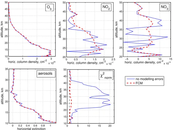
The e_ffect of including modeling errors into the inversion is illustrated in Fig. 1, first for the individual occultation of Sirius at the orbit 7673. It is known that the quality of inversion can be characterized with the normalizedχ2 statistics χ_norm2 =_Mχ₋2_P, where χ2 is defined by Eq. (1), M is the number of measurements and P is the number of retrieved parameters. If the model describes well the experimental data and the 15

measurement errors are properly defined,χnorm2 ≈1. If the modeling errors are ignored (i.e., the covariance matrix is takenC=C_noise),χ_norm2 can significantly exceed the value 1 in oblique occultations of bright stars; this indicates underestimation of the uncertainty of the retrieved densities. This is the case for the occultation shown in Fig. 1 (blue line). Inclusion of modeling errors reduces dramatically theχ_norm2 values (Fig. 1, red line). The 20

(10)

AMTD

3, 579–597, 2010

Title Page

Tables Figures

◭ ◮

Back Close

Full Screen / Esc

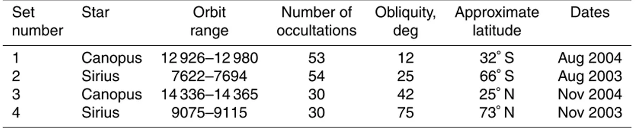
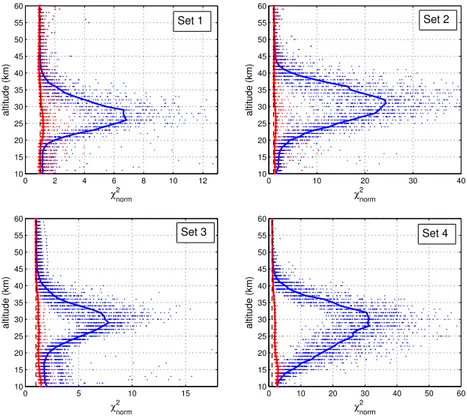
The features observed for the considered occultation of Sirius are common for oblique occultations of bright stars. Figure 2 shows theχ_norm2 values for four sets of suc-cessive oblique occultations of the brightest stars Sirius and Canopus. The information about these data sets is collected in Table 1. The GOMOS successive occultations of a certain star are located at approximately the same latitude, and they are carried out 5

at approximately the same local time. The values ofχ_norm2 dramatically decrease when modeling errors are taken into account (FCM method). They become close to the ideal valueχ_norm2 =1. This indicates that the parameterization of scintillation correction errors proposed in (Sofieva et al., 2009) properly describes the main source for modeling errors at altitudes_∼20₋50 km.

10

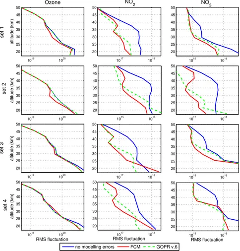
For characterization of smoothness of the retrieved horizontal column density pro-files, we consider the profile fluctuationsδN=N_−hN_i. The mean profile_hN_iis obtained by smoothing the original profiles with a rectangular window with the cut-off scale of 3 km. The altitude range was divided into segments of 5 km overlapping by 1 km. For each set of occultations, we computed rms of line density fluctuationsδN inside each 15

altitude segment. Rms fluctuations of the retrieved horizontal column density profiles are presented in Fig. 3, for retrievals without modeling error accounted in the inversion (blue lines) and for FCM inversion (red lines). The horizontal column density profiles become significantly smoother if the modeling errors are included into the inversion. The smoothing e_ffect is associated with the correlation of measurement uncertainties, 20

which is inherently taken into account in the FCM inversion (note that this is not regular-ization). The large unrealistic fluctuations in NO₂ and NO₃ profiles due to incomplete scintillation correction were noticed already in the first GOMOS data. In the current operational GOMOS retrievals (the IPF 5.0 processor), a variant of DOAS (di_ff eren-tial optical absorption spectroscopy) method, so called Global DOAS Iterative method 25

(11)

AMTD

3, 579–597, 2010

Title Page

Tables Figures

◭ ◮

Back Close

Full Screen / Esc

and NO₃profiles in the ”full covariance matrix” inversion is comparable to that obtained with the Global DOAS Iterative inversion. This highlights the importance of the correct characterization of modeling errors in the retrievals.

The proximity ofχnorm2 to 1 in the FCM inversion indicates that the characterization of the modeling errors is close to reality. At the same time, this ensures that the estimated 5

accuracy of the retrieved profiles is close to reality. The GOMOS spectral inversion is followed by the vertical inversion aimed at reconstruction of local density profiles from the collection of horizontal column densities (Kyr ¨ol ¨a et al., 2009; Sofieva et al., 2004). The vertical inversion is slightly noise-amplifying (i.e., the fluctuations existing in hori-zontal column density profile are enhanced after the vertical inversion) (Sofieva et al., 10

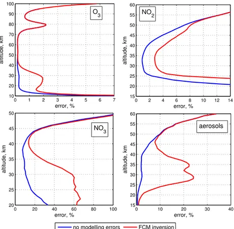
2004). An improved smoothness of the horizontal column density profiles obtained with FCM method is very advantageous therefore. In GOMOS processing, the Tikhonov-type regularization is applied in the vertical inversion for its stabilization (Tamminen et al., 2004; Sofieva et al., 2004). Figure 10 in Sofieva et al. (2009) shows the uncertainty estimates for the retrieved GOMOS ozone profiles, which include the characterization 15

of scintillation correction errors. In this paper, we discuss the changes in error es-timates due to including the modeling errors in the inversion. Figure 4 shows error estimates for local densities of O₃, NO₂, NO₃ and aerosols with ignored and included modeling errors in the inversion. If the modeling errors are ignored, the uncertainty of the retrieved profiles can be significantly underestimated for oblique occultations of 20

bright stars. For such occultations, the underestimation in uncertainty can achieve up to 1–2% for ozone, 2% for NO₂, 40 % for NO₃ and 15% for high-altitude aerosols (for aerosols below 20–25 km, the underestimation is significantly smaller, up to 7%). The altitude range of increased uncertainty corresponds to the range where the adverse in-fluence of scintillation correction error is maximal. This range depends on constituent 25

(12)

AMTD

3, 579–597, 2010

Title Page

Tables Figures

◭ ◮

Back Close

Full Screen / Esc

For dimmer stars, the percentage of modeling errors in the total error budget is smaller, therefore the underestimation of the resulting uncertainty of the retrieved pro-files is less remarkable. For vertical occultations, where the scintillation correction works nearly perfectly, including the modeling errors via FCM is not important (how-ever, such occultations constitute a small percent of the GOMOS data).

5

5 Discussion and summary

We have discussed inclusion of the modeling errors into the GOMOS inversion. For GOMOS, the main source of modeling errors at altitudes_∼20–50 km is the incomplete scintillation correction. The parameterization of scintillation correction errors proposed in (Sofieva et al., 2009), which adjusts “automatically” the magnitude and correlation 10

of the modeling errors to different occultation geometry, allows accurate quantifying modeling errors in this altitude range. While accounting the modeling errors, the inver-sion procedure based on non-linear minimization has to be optimized. The numerical efficiency is of high importance in the processing of satellite data, due to their large amount.

15

Our paper presents the algorithm for numerically efficient processing of GOMOS data, with modeling errors taken into account. It is based on using the Cholesky factor-ization and the subsequent change of variables. The “full covariance matrix” inversion was successfully implemented and tested on a large data set. Compared to the inver-sion without modeling errors, the following changes in inverinver-sion statistics and results 20

are observed:

1. Dramatic changes in normalizedχ2 values: fromχ_norm2 ∼20–50 in oblique occul-tations of bright stars toχ_norm2 _∼1–2, at altitudes 20–50 km. This ensures that the applied parameterization of scintillation correction errors proposed in (Sofieva et al., 2009) adequately describes the main source of modeling errors for altitudes 25

(13)

AMTD

3, 579–597, 2010

Title Page

Tables Figures

◭ ◮

Back Close

Full Screen / Esc

2. The horizontal column density profiles are smoother if the ”full covariance matrix” inversion is applied, especially for NO₂ and NO₃. This feature is advantageous for the GOMOS processing, as the subsequent vertical inversion is slightly noise-amplifying. The smoothness of NO₂ and NO₃ profiles becomes comparable to that obtained with the Global DOAS Iterative inversion (the current operational 5

GOMOS processing).

3. Significant increase of error bars (compared to the case of neglecting modeling errors) for oblique occultations of very bright stars is observed.

The main advantage of the “full covariance matrix” inversion is the proper charac-terization of the uncertainty of retrieved profiles. This feature is of high importance, 10

especially for validation, data assimilation and for time series analyses. The inversion method described in our paper is already implemented in next version of the GOMOS prototype processor (GOPR v.7), and it is planned to be used for future reprocessing of GOMOS data.

Acknowledgements. The work has been supported by ESA (ESRIN ESL Contract

15

N ˚ 21091/07/I-OL covering the GOMOS Software maintenance and evolution and support to CAL/VAL operations, led by ACRI-ST, with FMI, LATMOS, and IASB as Expert Support Labo-ratories partners). The work of V. Sofieva was supported by the Academy of Finland. The work of V. Kan was supported by RFBR grant 09-05-00180.

References 20

Dalaudier, F., Kan, V., and Gurvich, A. S.: Chromatic refraction with global ozone monitoring by occultation of stars, I, Description and scintillation correction, Applied Opt., 40, 866–877, 2001.

Hauchecorne, A., Bertaux, J.-L., Dalaudier, F., et al.: First simultaneous global measure-ments of nighttime stratospheric NO2 and NO3 observed by Global Ozone Monitoring by 25

(14)

AMTD

3, 579–597, 2010

Title Page

Tables Figures

◭ ◮

Back Close

Full Screen / Esc

Interactive Discussion Kyr ¨ol ¨a, E., Sihvola, E., Kotivuori, Y., Tikka, M., Tuomi, T., and Haario, H.: Inverse theory for

occultation measurements: 1. Spectral inversion, J. Geophys. Res., 98, 7367–7381, 1993. Kyr ¨ol ¨a, E., Tamminen, J., Sofieva, V. F., et al.: GOMOS retrieval algorithms, GOMOS special

issue, 2009.

Polyakov, A., Yu., V., Timofeev, M., Gurvich, A. S., Vorob’ev, V. V., Kan, V., and Yee, J.-H.: Effect

5

of Stellar Scintillations on the Errors in Measuring the Ozone Content of the Atmosphere, Izv., Atm. Ocean. Phys., 37(1), 51–60, 2001 (English translation).

Press, W. H., Teukolsky, S. A., Vetterling, W. T., and Flannery, B. P.: Numerical Recipes in FORTRAN, The Art of Scientific Computing, Clarendon Press, Oxford, 1992.

Sofieva, V. F., Tamminen, J., Haario, H., Kyr ¨ol ¨a, E., and Lehtinen, M.: Ozone profile smoothness

10

as a priori information in the inversion of limb measurements, Ann. Geophys., 22, 3411– 3420, 2004,

http://www.ann-geophys.net/22/3411/2004/.

Sofieva, V. F., Kyr ¨ol ¨a, E., Hassinen, S., et al.: Global analysis of scintillation variance: Indication of gravity wave breaking in the polar winter upper stratosphere, Geophys. Res. Lett., 34,

15

L03812, doi:10.1029/2006GL028132, 2007.

Sofieva, V. F., Kan, V., Dalaudier, F., Kyr ¨ol ¨a, E., Tamminen, J., Bertaux, J.-L., Hauchecorne, A., Fussen, D., and Vanhellemont, F.: Influence of scintillation on quality of ozone monitoring by GOMOS, Atmos. Chem. Phys., 9, 9197–9207, 2009,

http://www.atmos-chem-phys.net/9/9197/2009/.

20

(15)

AMTD

3, 579–597, 2010

Title Page

Tables Figures

◭ ◮

Back Close

Full Screen / Esc

Interactive Discussion Table 1.GOMOS occultations selected for the statistical analyses.

Set Star Orbit Number of Obliquity, Approximate Dates

number range occultations deg latitude

1 Canopus 12 926–12 980 53 12 32◦S Aug 2004

2 Sirius 7622–7694 54 25 66◦S Aug 2003

3 Canopus 14 336–14 365 30 42 25◦N Nov 2004

(16)

AMTD

3, 579–597, 2010

Title Page

Tables Figures

◭ ◮

Back Close

Full Screen / Esc

0 0.5 1 1.5 2 2.5

x 1017

20 25 30 35 40 45 50

altitude, km

horiz. column density, cm−2

−5 0 5 10 15

x 1014

20 25 30 35 40 45 50

altitude, km

0 0.2 0.4 0.6 0.8 1

10 15 20 25 30 35

altitude, km

horizontal extinction

0 5 10 15 20

10 15 20 25 30 35 40 45 50

altitude, km

no modelling errors FCM

0 1 2 3

x 1020

10 15 20 25 30 35 40 45 50

altitude, km

aerosols

O₃ NO₂ NO₃

χ2

norm

(17)

AMTD

3, 579–597, 2010

Title Page

Tables Figures

◭ ◮

Back Close

Full Screen / Esc

0 2 4 6 8 10 12

10 15 20 25 30 35 40 45 50 55 60

χ2 norm

altitude (km)

0 10 20 30 40

10 15 20 25 30 35 40 45 50 55 60

χ2 norm

altitude (km)

0 5 10 15

10 15 20 25 30 35 40 45 50 55 60

χ2 norm

altitude (km)

0 10 20 30 40 50 60

10 15 20 25 30 35 40 45 50 55 60

χ2 norm

altitude (km)

Set 1 Set 2

Set 3 Set 4

(18)

AMTD

3, 579–597, 2010

Title Page Abstract Introduction Conclusions References Tables Figures ◭ ◮ ◭ ◮ Back Close

Full Screen / Esc

1019 1020 20 25 30 35 40 45 50 Ozone altitude (km)

1017 1018 20 25 30 35 40 45 50 NO 2 set 1

1015 1016 20 25 30 35 40 45 50 NO 3

1019 1020 20 25 30 35 40 45 50 altitude (km)

1017 1018 20 25 30 35 40 45 50

1015 ₁₀16 20 25 30 35 40 45 50 set 2

1019 ₁₀20 20 25 30 35 40 45 50 altitude (km)

1017 1018 20 25 30 35 40 45 50 set 3

1019 1020 20 25 30 35 40 45 50 altitude (km) RMS fluctuation

1017 1018 20 25 30 35 40 45 50 RMS fluctuation set 4

1015 1016 20 25 30 35 40 45 50 RMS fluctuation no modelling errors FCM GOPR v.6

1015 1016 20 25 30 35 40 45 50

Fig. 3. Rms of horizontal column density fluctuations for different processing methods. Left column: ozone, middle column: NO2, right column: NO3. The rows correspond to the data sets

(19)

AMTD

3, 579–597, 2010

Title Page

Tables Figures

◭ ◮

Back Close

Full Screen / Esc

Interactive Discussion 0 1 2 3 4 5 6 7

10 20 30 40 50 60 70 80 90 100

altitude, km

error, %

0 2 4 6 8 10 12 14 15

20 25 30 35 40 45 50 55 60

altitude, km

error, %

0 20 40 60 80 100 20

25 30 35 40 45 50

altitude, km

error, %

0 10 20 30 40

15 20 25 30 35 40 45 50 55 60

altitude, km

error, %

no modelling errors FCM inversion O

3 NO2

NO

3 aerosols