Interannual variability and future projection of summertime ocean wave heights in the western North Pacific

(1)

OSD

3, 1637–1651, 2006

Wave height projection in the WNP

W. Sasaki et al.

Title Page

Abstract Introduction

Conclusions References

Tables Figures

◭ ◮

Back Close

Full Screen / Esc

Printer-friendly Version

Interactive Discussion

EGU

Ocean Sci. Discuss., 3, 1637–1651, 2006 www.ocean-sci-discuss.net/3/1637/2006/ © Author(s) 2006. This work is licensed under a Creative Commons License.

Ocean Science Discussions

Papers published inOcean Science Discussions_{are under}

open-access review for the journalOcean Science

Interannual variability and future

projection of summertime ocean wave

heights in the western North Pacific

W. Sasaki1, T. Hibiya2, and T. Kayahara1

1

Storm, Flood and Landslide Research Department, National Research Institute for Earth Science and Disaster Prevention, Tsukuba, Japan

2

Department of Earth and Planetary Science, Graduate School of Science, University of Tokyo, Tokyo, Japan

Received: 19 September 2006 – Accepted: 4 October 2006 – Published: 6 October 2006

(2)

OSD

3, 1637–1651, 2006

W. Sasaki et al.

Title Page

Tables Figures

◭ ◮

Back Close

Full Screen / Esc

EGU Abstract

A 70–yr (from 1985–1995 to 2055–2065) change of decadal mean summertime ex-treme significant wave heights (SWH) in the western North Pacific under CO2–induced global warming condition is projected. For this purpose, possible atmospheric fields under future global warming are derived from 10–yr time–slice experiments using a

5

T106 AGCM. The future changes of SWH are assessed by an empirical approach, where possible changes of SWH are estimated using a linear regression model which shows an empirical relationship between SWH anomalies and an eastward shift of the monsoon trough. It is projected that SWH increases by up to∼0.4 m over a wide area of the western North Pacific .

10

1 Introduction

Some of the state–of–the–art coupled climate models predict increase of the inten-sity of tropical cyclone (TC) and decrease of the frequency of TC under CO₂–induced global warming (Krishnamurti et al., 1998). Since the changes of TC intensity as well as TC frequency may cause changes of ocean wave climate, it is interesting to project

15

ocean wave heights in the area where the TC frequently develops.

Future changes of ocean wave heights were first projected by the Waves and Storms in the North Atlantic (WASA) Group (WASA, 1998). They carried out 5–yr time–slice experiments for the North Atlantic to present a statistical projection of intramonthly quantiles of ocean wave heights at Brent and near Ekofisk. They also presented a

20

dynamical projection of changes of ocean wave heights by driving the third–generation wave model using surface wind fields derived from the time–slice experiments. Wang et al. (2004) projected wave climate changes in the North Atlantic for the 21st century using sea level pressure fields derived from a global climate model under three different forcing scenarios. Recently, this method was applied to project seasonal averages and

25

(3)

OSD

3, 1637–1651, 2006

W. Sasaki et al.

Title Page

Tables Figures

◭ ◮

Back Close

Full Screen / Esc

EGU

for three forcing–scenarios (Wang and Swail, 2006). Moreover, they discussed the uncertainties in the projections of wave heights in terms of the differences among the three climate models as well as three forcing–scenarios.

In this paper, we present an empirical projection of a 70–yr (from 1985–1995 to 2055–2065) change of 10–yr mean summertime extreme significant wave heights in

5

the western North Pacific (WNP) under CO2–induced global warming condition. First, possible atmospheric fields under future global warming are derived from the time–slice experiments. Next, thus derived information is incorporated into the linear regression model which empirically relates the atmospheric fields to interannual variability of SWH.

2 Data and time–slice experiments 10

2.1 Reanalysis data and employed procedures

We use significant wave heights (SWH), surface wind (SW), and sea level pressure (SLP) fields covering the world ocean on a 2.5◦×2.5◦grid at 6–h intervals for September 1957–August 2002 obtained from the ERA–40 reanalysis, namely, a 40–yr reanalysis of the atmospheric and oceanic fields developed at the European Centre for Medium–

15

Range Weather Forecasts. We also use monthly mean sea surface temperature (SST) fields obtained from the Extended Reconstructed Sea Surface Temperature (ERSST) (Smith and Reynolds, 2004). From these datasets, we can obtain 3–month (June– August) averaged maps of the monthly 90th percentile of SWH (H90), SW, SLP, and SST for each year. However, we exclude H90in 1992 from the datasets since the ERA–

20

40 wave reanalysis has inhomogeneity during December 1991–May 1993 because of the assimilation of faulty ERS–1 Fast Delivery Product (Bauer and Staabs, 1998).

To obtain a regression model which relates dominant interannual variability of H90 to monthly mean atmospheric fields, we apply an Empirical Orthogonal Function (EOF) analysis to the above obtained 3–month averaged H₉₀ field for the region 0◦_N–40◦_N,

25

100◦_E–180◦_{based on the covariance matrix. The first EOF of H}

(4)

OSD

3, 1637–1651, 2006

W. Sasaki et al.

Title Page

Tables Figures

◭ ◮

Back Close

Full Screen / Esc

EGU

of the total variance within this region. The explained variance is 13.0% for the second mode and 5.5% for the third mode, both much smaller than that of the first mode, so that we focus only on the first EOF mode hereafter. To identify the H90, SST, and atmospheric anomalies associated with the first EOF mode of H90 in the WNP, we illustrate a map of linear regression coe_fficients between the principal component for

5

the first EOF mode (PC1) and each of H90, SST, SW, and SLP (Fig. 1).

For tropical cyclones (TCs), we use the TC best–track data issued by the Regional Specialized Meteorological Center (RSMC) Tokyo Typhoon Center as well as the TC best–track data from the U.S. Joint Typhoon Warning Center (JTWC).

2.2 Time–slice experiments

10

Present–day and future atmospheric fields are simulated by a pair of time–slice exper-iments (control run as well as 2×CO2 run) using an atmospheric general circulation model (AGCM). The employed AGCM is the global spectral model which has been used as the forecast model in the Japan Meteorological Agency (Sugi et al., 1990) and is the atmospheric component of a coupled ocean–atmosphere general circulation

15

model (CGCM) developed at the National Research Institute for Earth Science and Dis-aster Prevention (Matsuura et al., 1999; Iizuka et al., 2003). In this study, the AGCM is configured with the horizontal spectral truncation of T106, and 21 vertical levels.

In the control run where the carbon dioxide (CO2) concentration is fixed at 350 ppm, we integrate the AGCM for 11 years to reproduce the equilibrium response to

clima-20

tological SST fields for 1985–1995 derived from the ERSST. In the 2×CO2 run where the CO2 concentration is fixed at 700 ppm, we use climatological SST fields derived from the Greenhouse gases Plus Sulfates (GPS) experiments with a coarse–resolution (R30) CGCM developed at the Geophysical Fluid Dynamics Laboratory (Delworth et al., 2002). In the GPS experiments, CO2 concentration is assumed to increase at a

25

(5)

pos-OSD

3, 1637–1651, 2006

W. Sasaki et al.

Title Page

Tables Figures

◭ ◮

Back Close

Full Screen / Esc

EGU

sible SST field under CO₂–induced future global warming, the difference between SST for 2055–2065 and that for 1985–1995 is added to the observed SST; for the resulting SST field, the AGCM is integrated for 11 years.

We now examine TC activity in the control run using two different cumulus convec-tion schemes, namely, the KUO scheme proposed by Kuo (1974), and a prognostic

5

Arakawa–Schubert scheme modified by Kuma (1996) (the PAS scheme). Although both cumulus convection schemes are widely used for the time–slice experiments (Sugi et al., 2002; Oouchi et al., 2006; Yoshimura et al., 2006), it is interesting to see which convection scheme is favorable to reproduce TC activity similar to actually observed. Figure 2 shows the TC tracks calculated using the KUO and the PAS schemes together

10

with the observed ones. We can see that the TC frequency for the KUO scheme is much less than that for the PAS scheme and/or actually observed. Furthermore, TCs for the KUO scheme do not propagate up northward compared to the others. These results indicate that the PAS scheme is favorable to examine summertime WNP wave climate which strongly depends on TC activity. For this reason, we hereafter use only

15

calculated results from time–slice experiments with the PAS scheme.

The atmospheric fields derived from the time–slice experiments are used to assess possible future changes of SWH. We employ an empirical approach to project future changes of SWH, where the difference of surface winds (2×CO2run minus control run) is incorporated into the linear regression model which will be introduced in Sect. 3.

20

3 Results

3.1 Interannual variability of H90 in the WNP

The spatial structure of the first EOF mode for H90 is characterized by a monopole structure with the maximum amplitude located to the south of Japan (Fig. 1a). Time variations of the PC1 for H₉₀ (Fig. 1b) indicate that H₉₀ increases during the ENSO

25

(6)

OSD

3, 1637–1651, 2006

W. Sasaki et al.

Title Page

Tables Figures

◭ ◮

Back Close

Full Screen / Esc

EGU

with Sasaki et al. (2005a) who showed that monthly mean SWH offthe southern coast of Japan tends to increase during the ENSO years.

Typical atmospheric and oceanic anomalies associated with increase of H90 can be characterized by cyclonic circulation in the WNP in response to warm SST anomalies in the Ni ˜no–3.4 region (Figs. 1c and d). Table 1a provides the decennial correlation

5

coefficients between the SST averaged over the Ni ño–3.4 region (Ni ño–3.4 index) and the PC1 for H₉₀where we can see that the correlation between the Ni ño–3.4 index and the PC1 for H90 is low during 1960–1969 (r=−0.16), but is much improved after 1970 (r >0.5).

It is interesting to note that strong anomalous westerly winds can be found in the

10

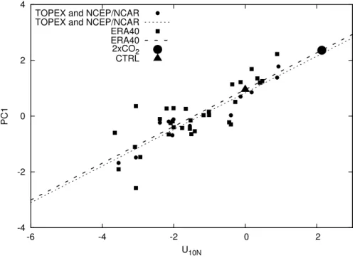
SW anomalies within the region 5◦_N–15◦_{N, 130}◦_E–160◦_{E. The time series of zonal} wind anomalies averaged over this region (U10N) coincides with that of the PC1 for H90 (Fig. 1b). In fact, Table 1b shows that U10Nand the PC1 for H90are positively correlated with each other after 1970 (r >0.7), thus validating the linear regression model which empirically predicts the PC1 for H90 in terms of U10N. A dashed line in Fig. 3 shows a

15

linear regression model which relates the PC1 for H90 to U10N, where we can see the linear relationship between the PC1 for H₉₀and U_10Nbased on the ERA–40 reanalysis. We can confirm the robust relationship between the PC1 for H90and U10Nbased on the other datasets. A dotted line in Fig. 3 shows a linear regression model which relates the PC1 of H₉₀ obtained from optimally interpolated TOPEX/Poseidon SWH to U_10N

20

obtained from the National Centers for Environmental Prediction – National Center for Atmospheric Research (NCEP–NCAR) reanalysis for 1993–2004 (Sasaki and Hibiya, 2006). Correlation coe_fficient between the PC1 for H₉₀ from the TOPEX/Poseidon SWH and U10Nfrom the NCEP–NCAR reanalysis is 0.95. Although small bias is found between the two regression models, their slopes are nearly identical. The robust

rela-25

tionship between the PC1 for H₉₀ and U_10Nthus confirmed enables us to use U_10Nas the predictor for the PC1 of H90.

(7)

OSD

3, 1637–1651, 2006

W. Sasaki et al.

Title Page

Tables Figures

◭ ◮

Back Close

Full Screen / Esc

EGU

of the occurrence of TCs. In fact, the mean position of the occurrence of TCs during the highest seven years of the PC1 for H90 shifts southeastward when compared to that during the lowest seven years of the PC1 for H90(Figures not shown), so that TCs may have longer duration until encountering the continent or cold mid–latitude water. Wang and Chan (2002) showed that, during the strong ENSO events, TC tends to

5

occur in the southeast quadrant (0◦_N–17◦_{N, 140}◦_E–180◦_{) with the intensity increasing} in proportion to its duration.

Table 1c shows that the PC1 for H90 is strongly correlated with the total duration of intense TC (ITC; TC with the central pressure below 980 hPa) computed from the RSMC best–track data. This is consistent with Sasaki et al. (2005b) who showed that,

10

in the WNP, summertime extreme ocean wave heights (defined as the June–August average of the highest 10 % for a month) and total duration of ITC both increase since the late 1990s. In contrast, we cannot recognize any apparent correlation between the TC frequency and the PC1 for H₉₀ (Table 1d). Poor correlations in the 1960s shown in Table 1a–d may reflect a data problem of TC best–track data as well as the ERA–40,

15

since the satellite monitoring of weather events in the WNP was not carried out before 1965.

3.2 Projected changes of H90in the WNP

To conduct empirical projection of future changes of H₉₀ in the WNP, we assume that the statistical relationship between the PC1 for H90 and U10N at present–day will hold

20

under the future climate condition. In the empirical approach, a 70–year change (from 1985–1995 to 2055–2065) of the 10–year mean of H₉₀ is estimated using a linear regression model shown in Fig. 3. A pair of time–slice experiments shows that calcu-lated U10N at present–day is somewhat larger than actually observed, and increases by∼2 ms−1 under CO2–induced global warming condition (Fig. 3). Spatial pattern of

25

(8)

Consid-OSD

3, 1637–1651, 2006

W. Sasaki et al.

Title Page

Tables Figures

◭ ◮

Back Close

Full Screen / Esc

EGU

ering that future SST fields employed in the 2×CO2run exhibit ENSO–like features, en-hancement of U10Nthus projected in the WNP is quite natural. Possible future changes of H90can be estimated by incorporating the projected U10Ninto the regression model. We can see that the projected H₉₀ increases by up to∼0.4 m over a wide area of the WNP (Fig. 4).

5

4 Conclusions

We have presented a 70–year change (from 1985–1995 to 2055–2065) of the 10–year mean of H90 in the western North Pacific under the GPS experiments in which CO2 concentration is assumed to increase at a rate following the IS92a scenario until 1990, and at a rate 1% per year thereafter. For this purpose, we have conducted 10–yr time–

10

slice experiments using T106 AGCM. Future projection has been carried out through an empirical approach using the possible atmospheric fields derived from the time– slice experiments. It has been projected that H₉₀ increases by up to ∼0.4 m over a wide area of the western North Pacific.

References 15

Bauer, E. and Staabs, C.: Statistical properties of global significant wave heights and their use for validation, J. Geophys. Res., 103(C1), 1153–1166, 1998.

Delworth, T. L., Stouffer, R. J., Dixon, K. W., Spelman, M. J., Knutson, T. R., Broccoli, A. J., Knushner, P. J., and Wetherald, R. T.: Review of simulations of climate variability and change with GFDL R30 coupled climate model, Clim. Dyn., 19, 555–574, 2002.

20

Iizuka, S., Orito, K., Matsuura, T., and Chiba, M.: Influence of cumulus convection schemes on the ENSO–like phenomena simulated in a CGCM, J. Meteorol. Soc. Japan, 81, 85–827, 2003.

Krishnamurti, T. N., Correa-Torres, R., Latif, M., and Daughenbaugh, G.: The impact of current and possibly future SST anomalies on the frequency of Atlantic hurricanes, Tellus, 50A, 186–

25

(9)

OSD

3, 1637–1651, 2006

W. Sasaki et al.

Title Page

Tables Figures

◭ ◮

Back Close

Full Screen / Esc

EGU

Kuma, K.: Parameterization of cumulus convection, JMA/NPD Report No. 42, 93pp, 1996. Kuo, H. L.: Further studies of the influence of cumulus convection on large scale flow, J. Atmos.

Sci., 31, 1232–1240.

Matsuura, T., Yumoto, M., Iizuka, S., Kawamura, R.: Typhoon and ENSO simula-tion using a high-resolusimula-tion coupled GCM, Geophys. Res. Lett., 26(12), 1755–1758,

5

doi:10.1029/1999GL900329, 1999.

Oouchi, K., Yoshimura, J., Yoshimura, H., Mizuta, R., Kusunoki, S., and Noda, A.: Tropical cyclone climatology in a global–warming climate as simulated in a 20 km–mesh global atmo-spheric model: frequency and wind intensity analyses, J. Meteorol. Soc. Japan, 84, 259–276, 2006.

10

Sasaki, W., Iwasaki, S. I., Matsuura, T., Iizuka, S., and Watabe, I.: Changes in wave climate off Hiratsuka, Japan, as affected by storm activity over the western North Pacific, J. Geophys. Res., 110, C09008, doi:10.1029/2004JC002730, 2005a.

Sasaki, W., Iwasaki, S. I., Matsuura, T., and Iizuka, S.: Recent increase in summertime extreme wave heights in the western North Pacific, Geophys. Res. Lett., 32, L15607,

15

doi:10.1029/2005GL023722, 2005b.

Sasaki, W. and Hibiya, T.: Interannual variability and predictability of summertime significant wave heights in the western North Pacific, J. Oceanogr., in press, 2006.

Smith, T. M. and Reynolds, R. W.: Improved extended reconstruction of SST (1854–1997), J. Clim., 17, 2466–2477, 2004.

20

Sugi, M., Kuma, K., Tada, K., Tamiya, K., Hasegawa, N., Iwasaki, T., Yamada, S., and Kitade, T.: Description and performance of the JMA operational global spectral model (JMA–GSM88), Geophys. Mag., 43, 105–130, 1990.

Sugi, M., Noda, A., and Sato, N.: Influence of the global warming on tropical cyclone clima-tology: An experiment with the JMA global model, J. Meteorol. Soc. Japan, 80, 249–272,

25

2002.

Tolman, H. L.: User manual and system documentation of WAVEWATCH-III version 1.18, NOAA/NWS/NCEP Ocean Modeling Branch Contribution 166, 112pp, 1999.

Wang, B. and Chan, J. C. L.: How strong ENSO events a_ffect tropical storm activity over the western North Pacific, J. Clim., 15, 1643–1658, 2002.

30

Wang, X. L., Zwiers, F. W., and Swail, V. R.: North Atlantic ocean wave climate change scenar-ios for the twenty–first century, J. Clim., 17, 2368–2383, 2004.

(10)

OSD

3, 1637–1651, 2006

W. Sasaki et al.

Title Page

Tables Figures

◭ ◮

Back Close

Full Screen / Esc

EGU

wave heights, Clim. Dyn., 26, 109–126, doi:10.1007/s00382-005-0080-x, 2006.

WASA Group: Changing waves and storms in the northeast Atlantic?, Bull. Amer. Meteorol. Soc., 79, 741–760, 1998.

Yoshimura, J., Sugi, M., and Noda, A.: Influence of greenhouse warming on tropical cyclone frequency, J. Meteorol. Soc. Japan, 84, 405–428, 2006.

(11)

OSD

3, 1637–1651, 2006

W. Sasaki et al.

Title Page

Tables Figures

◭ ◮

Back Close

Full Screen / Esc

EGU Table 1.Decennial correlation coe_fficients between the PC1 for H₉₀in the western North Pacific

and (a) the Ni ˜no–3.4 index, (b) U_10N, (c) total duration of ITC, and (d) TC frequency.

Period

1960–1969 1970–1979 1980–1989 1990–2002 1960–2002

(12)

OSD

3, 1637–1651, 2006

W. Sasaki et al.

Title Page

Tables Figures

◭ ◮

Back Close

Full Screen / Esc

EGU Fig. 1. (a)A map showing the linear regression coefficients between H₉₀and the PC1 for H₉₀.

(13)

OSD

3, 1637–1651, 2006

W. Sasaki et al.

Title Page

Tables Figures

◭ ◮

Back Close

Full Screen / Esc

EGU Fig. 2. TC tracks from the observation (top), the control run using the PAS scheme (middle),

(14)

OSD

3, 1637–1651, 2006

W. Sasaki et al.

Title Page

Tables Figures

◭ ◮

Back Close

Full Screen / Esc

EGU -4

-2 0 2 4

-6 -4 -2 0 2

PC1

U_10N TOPEX and NCEP/NCAR

TOPEX and NCEP/NCAR ERA40 ERA40 2xCO₂ CTRL

Fig. 3. Relationship between the PC1 for H₉₀in the western North Pacific and U_10N obtained from the ERA–40 reanalysis (square) as well as from the TOPEX/Poseidon and the NCEP– NCAR reanalysis (circle). Our regression model is represented by a straight line obtained from the least square fit. The dashed line is for the ERA–40 reanalysis, whereas the dotted line is for the TOPEX/Poseidon and the NCEP–NCAR reanalysis. The triangle shows the PC1 for H₉₀projected by U_10Nderived from the control run, whereas the large circle shows the PC1 for H₉₀projected by U_10N derived from the 2×CO2run (both projections are carried out using the

(15)

OSD

3, 1637–1651, 2006

W. Sasaki et al.

Title Page

Tables Figures

◭ ◮

Back Close

Full Screen / Esc

EGU Fig. 4. A projected 70–year change (2055–2065 minus 1985–1995) of the 10–year mean of

H₉₀. Unit is m. Arrow shows the difference between surface wind vector obtained from the 2×CO2run and that obtained from the control run. Unit of wind speed is ms−

1