www.biogeosciences.net/10/4037/2013/ doi:10.5194/bg-10-4037-2013
© Author(s) 2013. CC Attribution 3.0 License.
Biogeosciences
Geoscientiic
Geoscientiic
Geoscientiic
Geoscientiic
Sea–air CO
2
fluxes in the Southern Ocean for the period 1990–2009
A. Lenton1, B. Tilbrook1,2, R. M. Law3, D. Bakker4, S. C. Doney5, N. Gruber6, M. Ishii7, M. Hoppema8, N. S. Lovenduski9, R. J. Matear10, B. I. McNeil11, N. Metzl12, S. E. Mikaloff Fletcher13, P. M. S. Monteiro14, C. R¨odenbeck15, C. Sweeney16, and T. Takahashi17
1Centre for Australian Weather and Climate Research, CSIRO Marine and Atmospheric Research, Hobart, Tasmania,
Australia
2Antarctic Climate Ecosystems Co-operative Research Centre, Hobart, Tasmania, Australia
3Centre for Australian Weather and Climate Research, CSIRO Marine and Atmospheric Research, Aspendale, Victoria,
Australia
4School of Environmental Sciences, University of East Anglia Research Park, Norwich NR4 7TJ, UK
5Marine Chemistry and Geochemistry Dept., Woods Hole Oceanographic Institution, Woods Hole, MA 02543, USA 6Institute of Biogeochemistry and Pollutant Dynamics and Center for Climate Systems Modeling, ETH Zurich, Zurich,
Switzerland
7Meteorological Research Institute, Tsukuba 305-0031, Japan 8Alfred Wegener Institute, Bremerhaven, Germany
9Department of Atmospheric and Oceanic Sciences, Institute of Arctic and Alpine Research, University of Colorado, Boulder,
CO 80309, USA
10Centre for Australian Weather and Climate Research, CSIRO Marine and Atmospheric Research, Hobart, Tasmania,
Australia
11Climate Change Research Centre, University of New South Wales, Sydney, Australia
12Laboratoire d’Oc´eanographie et du Climat, LOCEAN/IPSL, CNRS, Universit´e Pierre et Marie Curie, Paris, France 13National Institute of Water and Atmospheric Research, Wellington 6021, New Zealand
14Department of Oceanography, University of Cape Town, Rondebosch 7700, South Africa and Ocean Systems & Climate
Group, CSIR, Stellenbosch, South Africa
15Max-Planck-Institute for Biogeochemistry, 07745 Jena, Germany
16Cooperative Institute for Research in Environmental Science, University of Colorado, Boulder, CO 80305, USA 17Lamont-Doherty Earth Observatory of Columbia University, Palisades, New York, USA
Correspondence to:A. Lenton (andrew.lenton@csiro.au)
Received: 27 November 2012 – Published in Biogeosciences Discuss.: 8 January 2013 Revised: 1 May 2013 – Accepted: 9 May 2013 – Published: 19 June 2013
Abstract. The Southern Ocean (44–75◦S) plays a critical role in the global carbon cycle, yet remains one of the most poorly sampled ocean regions. Different approaches have been used to estimate sea–air CO2fluxes in this region:
syn-thesis of surface ocean observations, ocean biogeochemical models, and atmospheric and ocean inversions. As part of the RECCAP (REgional Carbon Cycle Assessment and Pro-cesses) project, we combine these different approaches to quantify and assess the magnitude and variability in South-ern Ocean sea–air CO2 fluxes between 1990–2009. Using
all models and inversions (26), the integrated median
an-nual sea–air CO2flux of−0.42±0.07 Pg C yr−1for the 44–
75◦S region, is consistent with the−0.27±0.13 Pg C yr−1
calculated using surface observations. The circumpolar re-gion south of 58◦S has a small net annual flux (model and inversion median:−0.04±0.07 Pg C yr−1and observations: +0.04±0.02 Pg C yr−1), with most of the net annual flux
lo-cated in the 44 to 58◦S circumpolar band (model and in-version median: −0.36±0.09 Pg C yr−1 and observations:
of 11 atmospheric inversions shows little seasonal change in the net flux. South of 58◦S, neither atmospheric inversions nor ocean biogeochemical models reproduce the phase and amplitude of the observed seasonal sea–air CO2flux,
partic-ularly in the Austral Winter. Importantly, no individual atmo-spheric inversion or ocean biogeochemical model is capable of reproducing both the observed annual mean uptake and the observed seasonal cycle. This raises concerns about project-ing future changes in Southern Ocean CO2fluxes. The
me-dian interannual variability from atmospheric inversions and ocean biogeochemical models is substantial in the Southern Ocean; up to 25 % of the annual mean flux, with 25 % of this interannual variability attributed to the region south of 58◦S. Resolving long-term trends is difficult due to the large interannual variability and short time frame (1990–2009) of this study; this is particularly evident from the large spread in trends from inversions and ocean biogeochemical models. Nevertheless, in the period 1990–2009 ocean biogeochem-ical models do show increasing oceanic uptake consistent with the expected increase of−0.05 Pg C yr−1decade−1. In
contrast, atmospheric inversions suggest little change in the strength of the CO2sink broadly consistent with the results
of Le Qu´er´e et al. (2007).
1 Introduction
Over recent decades, the ocean has taken up about 25 % of the annual anthropogenic CO2emissions to the atmosphere
from fossil fuel burning, cement production, and land-use change (Le Qu´er´e et al., 2009), slowing the growth of at-mospheric CO2 and therefore the rate of climate change.
The Southern Ocean, defined here as the oceanic region south of 44◦S, is a key region in the global uptake of anthropogenic CO2 (Caldeira and Duffy, 2000; Mikaloff
Fletcher et al., 2006). This region accounts for about one-third of the total global ocean uptake of anthropogenic CO2
(c.a. 0.7 Pg C yr−1), even though it covers less than 20 % of the global ocean surface area (Mikaloff Fletcher et al., 2006; Gruber et al., 2009). This uptake flux of anthropogenic CO2
is partially compensated by the degassing of natural CO2
(Mikaloff Fletcher et al., 2007), so that the contemporary up-take is smaller than that of anthropogenic CO2alone
(Taka-hashi et al., 2009). Projections suggest that the region will continue to be an important sink of atmospheric CO2,
al-though the efficiency of the sink may decrease (Roy et al., 2011). Despite its importance, the Southern Ocean remains one of the most poorly sampled ocean regions with respect to carbon dioxide (Monteiro et al., 2010; Fig. 2).
The Southern Ocean is dominated by the eastward flow-ing Antarctic Circumpolar Current (ACC). A northward Ekman transport at the surface of the ACC creates a di-vergence driven upwelling of carbon-rich water near the southern boundary of the ACC. The upwelling of
mid-STF SAF
PF
Fig. 1.Subregions of the Southern Ocean (44 to 75◦S) used in this
paper are the circular region 44–58◦S (green, red and blue
com-bined) and the major ocean basins (Pacific, Indian and Atlantic)
in this band, and the circumpolar region from 58–75◦S (purple).
Overlain is the network of atmospheric observations of CO2. The
colour of the dot indicates how many inversions used data from that location (dark grey: all or almost all inversions, light grey: around half the inversions, white: one or two inversions). We note that the temporal period over which the data was collected is not the same in all the stations. Overlain on these figures, from north to south are the mean positions of the major fronts subtropical front (STF), Subantarctic front (SAF) and the Polar Front (PF) following Orsi et al. (1995).
depth (2–2.5 km) water creates a unique connection between the deep ocean and the atmosphere, while the subduction of mode and intermediate waters further north links the Southern Ocean with waters that resurface at low latitudes (Sarmiento et al., 2004). The connections between the sur-face and ocean interior make the Southern Ocean an im-portant region for controlling ocean–atmosphere carbon ex-change and are a major influence in setting atmospheric CO2
levels (Sallee et al., 2012).
1191$
1192$ Fig. 2. The upper figure shows the location of observations of
oceanicpCO2. Black dots indicate the database (∼1 millionpCO2
measurement) used for Takahashi et al. (2002); and red dots
in-dicate an additional∼3 million data points used for Takahashi et
al. (2009). The lower panel shows the number of months of the year for which observations exist. This data is the basis of the obser-vational data used in this study (reproduced from Takahashi et al., 2009).
The available observations indicate that the seasonal cy-cle is the dominant mode of variability in the surface partial pressure of CO2 (pCO2)and the sea–air exchange for the
Southern Ocean (Lenton et al., 2006; Thomalla et al., 2011). Oceanic uptake of CO2from the atmosphere corresponds to a
negative net sea–air CO2flux, and an oceanic source of CO2
to the atmosphere has a positive net sea–air flux. Increased biological production in summer tends to reduce thepCO2
and increase the net ocean uptake of CO2. Lower biological
production and deeper mixing that entrains more CO2-rich
water into the mixed layer has the opposite effect in win-ter. Seasonal temperature changes offset the biological and mixing related effects on surfacepCO2and act to mute the
variability in seasonal sea–air fluxes (e.g. Takahashi et al., 2002 and Takahashi et al., 2009). While the biological and physical mechanisms driving this seasonal variability are rel-atively well known, their magnitude and phase remain poorly constrained (Metzl et al., 2006; Lenton et al., 2006).
In the austral summer the PFZ and SAZ act as strong sinks of atmospheric CO2due to enhanced biological production
(Metzl et al., 1999; Takahashi et al., 2009, 2012). In the
Aus-tral Winter, the net uptake of CO2in the PFZ and SAZ is
re-duced relative to summer, and in some areas a net outgassing occurs as a result of deep winter mixing entraining carbon-rich waters from the ocean interior into the surface mixed layer. When integrated annually, these regions act as a strong net sink of atmospheric CO2,with the largest uptake occur-ring in the SAZ and decreasing southward (Metzl et al., 1999, 2006; McNeil et al., 2007; Takahashi et al., 2012).
The AZ to the south of the PFZ contains a permanently ice free region in the north that transitions poleward to wa-ters covered seasonally by sea ice with some permanently ice-covered waters at high latitudes. The seasonal ice cov-ered region in the south portion of the AZ acts as a sink of atmospheric CO2in summer as sea-ice retreats and increased
stratification of the upper water column and greater light availability leads to an increase in the biological drawdown of carbon (Ishii et al., 1998; Bakker et al., 2008). Sea-ice cover inhibits sea–air gas exchange in winter, although there is considerable uncertainty as to how the ice cover impacts sea–air fluxes at high latitudes in winter months (e.g. Rys-gaard et al., 2011 and Loose and Schlosser, 2011). In the per-manently ice free region of the AZ,pCO2tends to be lower
than the atmosphere in summer owing to net biological pro-duction (Ishii et al., 2002; Metzl et al., 2006; Sokolov, 2008) and higher than the atmosphere in winter due to deep winter mixing. Integrated annually, the observations suggest the AZ acts as a neutral or weak source of atmospheric CO2
(Taka-hashi et al., 2009).
In recent decades, a strengthening of the Southern Annu-lar Mode (SAM), driven by increasing greenhouse gases and stratospheric ozone depletion, has resulted in a southward shift and intensification of the zonal winds, and increases in heat and freshwater fluxes over the Southern Ocean (Thomp-son and Solomon, 2002). During this period, oceanicpCO2
growth rates based on limited observations (Metzl, 2009; Takahashi et al., 2009) and some atmospheric inversions and ocean biogeochemical models (Le Qu´er´e et al., 2007) have suggested a decrease in the efficiency of the Southern Ocean CO2sink in response to these physical changes. The
strengthening SAM is believed to increase the upwelling of carbon-rich deep water that results in a decrease in the net ocean carbon uptake due to a change in the sea–air gradi-ent inpCO2(Le Qu´er´e et al., 2007; Lovenduski et al., 2007;
Lenton and Matear, 2007; Lenton et al., 2009). The corre-sponding changes in primary productivity are small relative to the response of ocean dynamics (Lenton et al., 2009). Fur-thermore, this change may have enhanced the outgassing of natural CO2 and had only a small effect on the uptake of
anthropogenic CO2 (Lovenduski et al., 2008; Matear and
Lenton, 2008). Evidence for a reduced efficiency of the Southern Ocean sink is not supported by all atmospheric in-versions (e.g. Law et al., 2008). Analyses of long-running atmospheric CO2 time series in the Southern Hemisphere
from atmospheric CO2measurements at present (Stephens et
al., 2013). Furthermore, ocean observations also suggest the changes in the sink efficiency may not be zonally uniform for the Southern Ocean (Lenton et al., 2012).
Different approaches have been used to estimate the to-tal sea–air CO2 fluxes (i.e. the anthropogenic+natural (or
pre-industrial)) in the Southern Ocean, including (i) syn-thesis of surface ocean pCO2 observations with
empiri-cal gas exchange parameterizations, and using interpolation schemes applied to ocean pCO2 observations to address
sparse data coverage; (ii) prognostic ocean biogeochemical models based on physical ocean general circulation models coupled with biogeochemical models; (iii) atmospheric in-version studies, based on the inin-version of atmospheric CO2
data; and (iv) ocean inversion models, based on ocean in-terior measurements and ocean model simulations. Histor-ically, these modelling approaches have produced signifi-cantly different annual mean estimates of Southern Ocean sea–air fluxes of carbon (e.g. Roy et al., 2003). A more re-cent study suggests there is growing agreement in the mag-nitude of the annual flux for the region (Gruber et al., 2009), although substantial differences remain with regard to the meridional distribution.
In this study we compare the total sea–air CO2fluxes in the
Southern Ocean derived from observations, atmospheric and ocean inverse calculations, and ocean biogeochemical mod-els for the period 1990–2009. The oceanic exchange of CO2
with the atmosphere through sea–air gas flux is driven by the difference in1pCO2 between the ocean and the overlying
atmosphere and is a function of wind-speed.
The goals of this work are to (i) quantify the annual sea–air flux of CO2; (ii) assess the sea–air flux and its relationship
with the annual mean uptake; (iii) quantify the magnitude of interannual variability in the Southern Ocean and investi-gate the long-term trends of ocean carbon uptake. This work is part of the REgional Carbon Cycle Assessment and Pro-cesses project (RECCAP; Canadell et al., 2011) led by the Global Carbon Project, and this paper is part of a special vol-ume of papers assessing the variability in the global carbon cycle over the period 1990–2009.
2 Methods
2.1 Datasets
The regional sea–air CO2fluxes described below use
REC-CAP “Tier 1” global CO2 flux products (Canadell et al.,
2011). These products include datasets of CO2 fluxes from
observations, ocean biogeochemical models, atmospheric and ocean inversions.
2.1.1 Observations
The Southern Ocean remains one of the most poorly sam-pled ocean regions with respect to carbon (Fig. 2), with some regions in the eastern South Pacific yet to be sam-pled. To account for this paucity of sampling, Takahashi et al. (2009) compiled more than 3 million measurements of oceanicpCO2 globally, and corrected these to the
refer-ence of the year 2000. These values were averaged onto a global grid, and two dimensional advection-diffusion equa-tions were used to interpolate spatially for each month (hashi et al., 1997). Wanninkhof et al. (2013) used the Taka-hashi gridded data and Calibrated Multi-Platform Winds (CCMP; Atlas et al., 2011) to generate a monthly 1◦×1◦
climatology of net sea–air CO2fluxes for RECCAP. In our
subsequent analysis and comparison with different models and inversions, we define observations as this climatology.
The steep meridional gradients in physical, chemical and biological properties of the Southern Ocean, as well as the patchiness of biological activities, means that the observed pCO2values vary over a wide range in space and time. This
combined with errors associated with sparse data coverage, wind speed measurements and gas transfer coefficients (for more discussion see Wanninkhof et al., 2013 and Sweeney et al., 2007) mean that the observationally derived fluxes con-tain large uncercon-tainties. Therefore, we conservatively esti-mated an uncertainty on all sea–air CO2 flux observations
of±50 %, consistent with Gruber et al. (2009) and Schuster
et al. (2013). There is insufficient observational data to as-sess the longer-term (interannual to decadal) variability for the entire Southern Ocean, and comparisons of model simu-lations and observed fluxes are limited in the following sec-tions to the annual and seasonal variability of the total (an-thropogenic and preindustrial) net sea–air CO2fluxes.
2.1.2 Ocean biogeochemical models
The simulated sea–air CO2 fluxes come from five ocean
general circulation models coupled to ocean biogeochemi-cal models (Table 1). These models represent the physibiogeochemi-cal, chemical and biological processes governing the marine car-bon cycle and the exchange of CO2 with the atmosphere.
All of these are z-coordinate models of coarse resolution that do not resolve or permit mesoscale eddies. The simulations were driven with observed reanalysis products for atmo-spheric boundary conditions over the period 1990–2009. All of these models have been integrated from the pre-industrial to present day with the same atmospheric CO2history. The
Table 1.Ocean biogeochemical models used this the study, their respective surface areas between 44◦S and 75◦S, the periods over which the data was evaluated, and the reference to each model.
Model Name Period Area (km2) Forcing Gas Exchange Ecosystem Limiting Nutrient Sea ice Reference structure
CSIRO 1990–2009 6.154×10⁷ NCEP–R1 Wanninkhof (1992) none (nutrient- P No Matear and Lenton (2008) restoring model)
CCSM-BEC 1990–2009 6.102×10⁷ NCEP–R1 Wanninkhof (1992) 4 phytoplankton+ N, P, Si, Fe Yes Thomas et al. (2008) 1 zooplankton
NEMO- 1990–2009 6.217×10⁷ NCEP–R1 Wanninkhof (1992) 2 phytoplankton+ N, P, Si, Fe Yes Le Qu´er´e et al. (2007)
PlankTOM5 2 zooplankton
NEMO-PISCES 1990–2009 6.102×10⁷ NCEP–R1 Wanninkhof (1992) 3 phytoplankton+ N, P, Si, Fe Yes Aumont and Bopp (2006) 2 zooplankton
CCSM-ETH 1990–2007 6.140×10⁷ CORE–2 Wanninkhof (1992)∗ 4 phytoplankton+ N, P, Si, Fe Yes Graven et al. (2012)
1 zooplankton
∗With a coefficient of 0.24 cm h−1s2m−2.
2.1.3 Atmospheric inversions
Inversions of atmospheric CO2measurements use an
atmo-spheric transport model and an optimization technique to de-termine carbon fluxes that best fit the atmospheric measure-ments. In most cases, a first guess or a priori flux based on independent datasets or models is also used to further con-strain the flux estimates. Here we use the same set of atmo-spheric CO2inversions as described in Peylin et al. (2013).
The inversions (Table 2) vary in many aspects, such as the at-mospheric transport model, sea–air CO2flux resolution,
so-lution method, a priori estimates and the atmospheric CO2
datasets.
In this study, we consider inversions that solve for carbon fluxes at a variety of different spatial resolutions, dividing the Southern Ocean region into between 1 and 14 regions or, in some cases, solving at the resolution of the transport model used in the inversion. In cases where inversions solved for regions that cross the 44◦S boundary used in this analysis, a proportion of the estimated flux is used, based on any as-sumptions about the flux distribution within a region. For the inversions solving at grid-cell resolution, those methods use a correlation length scale to ensure relatively smoothly vary-ing fluxes.
Figure 1 shows atmospheric-CO2measurement sites south
of 30◦S that were used by the inversions. Most sites were used by all or almost all the inversions, while Amsterdam Island (78◦E, 37◦S), Baring Head (175◦E, 41◦S) and ship data (169◦E, 30◦S) were used by only about half the in-versions (grey circles). There are three sites that are only used by one or two inversions. Many inversions use monthly mean atmospheric concentrations derived from the pseudo-weekly filtered data from the GLOBALVIEW-CO2 data
product (e.g. GLOBALVIEW-CO2, 2011 and earlier annual
releases). Four inversions use “raw” data (i.e. the inversions include flask observations at the appropriate sampling time) or hourly observations if these are available, though gener-ally with some selection based on time of day. All but three
inversions account for interannual variations in atmospheric transport.
An important consideration when interpreting the inverse estimates is to understand the influence of any prior infor-mation used in the inversion. For example, in almost all the inversions considered here, ocean CO2fluxes derived from
pCO2 measurements (e.g. Takahashi et al., 1999 or
Taka-hashi et al., 2009) were used to constrain the sea–air fluxes, so that the inversion is actually estimating sea–air fluxes that are deviations from the prior Takahashi-based estimates. De-pending on the spatial resolution of the inversion and the ad-ditional constraints that have been incorporated into the in-version, the basin-scale flux information may be strongly de-pendent on the prior information rather than new indede-pendent information derived from the local atmospheric CO2
mea-surements.
2.1.4 Ocean inversions
In this paper we use ten ocean inverse model simulations presented in Gruber et al. (2009) and the mean value across these simulations calculated from three periods: 1995, 2000 and 2005. As this technique only solves for an annual mean state, i.e. does not resolve seasonality or interannual vari-ability, these simulations are only used to assess the annual uptake. The specific details on methods and models used in these ocean inversions are detailed in Mikaloff Fletcher et al. (2006, 2007) and Gruber et al. (2009).
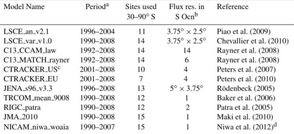
Table 2.Atmospheric inverse models and periods over which data was evaluated in this study, the number of sites south of 30◦S, model resolution and the reference to each model.
Model Name Perioda Sites used Flux res. in Reference
30–90◦S S Ocnb
LSCE an v2.1 1996–2004 11 3.75◦×2.5◦ Piao et al. (2009)
LSCE var v1.0 1990–2008 14 3.75◦×2.5◦ Chevallier et al. (2010)
C13 CCAM law 1992–2008 14 14 Rayner et al. (2008)
C13 MATCH rayner 1992–2008 14 6 Rayner et al. (2008)
CTRACKER USc 2001–2008 10 4 Peters et al. (2007)
CTRACKER EU 2001–2008 7 4 Peters et al. (2010)
JENA s96 v3.3 1996–2008 13 5◦×3.75◦ R¨odenbeck (2005)
TRCOM mean 9008 1990–2008 12 1 Baker et al. (2006)
RIGC patra 1990–2008 12 2 Patra et al. (2005)
JMA 2010 1990–2008 15 1 Maki et al. (2010)
NICAM niwa woaia 1990–2007 15 1 Niwa et al. (2012)d
aPeriod used for analysis. Inversions may have been run for a longer time.
bLongitude×latitude if inversion solves for each grid cell, otherwise number of ocean regions south of 44◦S. cCT2009 release.
dInversion method as this reference, except CONTRAIL aircraft CO
2data not used for RECCAP inversion.
The skill score weighting has a relatively minor influence on fluxes over most of the ocean. However, in the Southern Ocean, the skill score weighting leads to a smaller net uptake of CO2 by the Southern Ocean and a different distribution
of the uptake between regions. This is because some models used in the ocean inversion tend to overestimate CFC concen-trations in the Southern Ocean relative to observations, and also estimate substantially higher anthropogenic CO2uptake
in the inversion compared with other contributing models (Mikaloff Fletcher et al., 2006). The skill score-weighting scheme reduces the impact of these models on the weighted mean and therefore leads to a smaller estimated sink. 2.2 Study region
Following RECCAP protocols and its regional definitions, we use the latitudinal boundaries of 44–58◦S and 58–75◦S to define two broad Southern Ocean subdomains (Mikaloff Fletcher et al., 2006). The 44–58◦S circumpolar band in-cludes a large part of the SAZ and the PFZ, while the south-ern region includes the AZ. The region 44–58◦S is further split into the three major ocean basins: Indian, Pacific and At-lantic (Fig. 1; Table 3). All together we consider 6 regions in the Southern Ocean (Table 3): the five outlined above and one region comprising the total Southern Ocean south of 44◦S. 2.3 Calculation and assessment of sea–air CO2fluxes
The sea–air CO2fluxes for ocean models and inversions were
calculated as a median and the variability as a median abso-lute deviation (MAD; Gauss, 1816), consistent with Schuster et al. (2013). The MAD is the value where one half of all values are closer to the median than the MAD, and is a use-ful statistic for excluding outliers in datasets. The calculation of the annual uptake and seasonal variability of sea–air CO2
fluxes from atmospheric inversions and ocean biogeochem-ical models used data from all of the models and inversions listed in Tables 1 and 2. The seasonality in the sea–air CO2
flux calculated from the individual models was compared to net flux estimates from the surface ocean CO2 climatology
for the year 2000 using 2-quadrant Taylor diagrams (Taylor, 2001). This allows both the phase and magnitude of the sea-sonal cycle for each model to be assessed individually along with the annual mean value. Finally, in the calculation of trends we only used model simulations in which 10 or more years of output was available and assumed the trends were linear following Le Qu´er´e et al. (2007). The sea–air CO2flux
into the ocean is defined as negative, consistent with REC-CAP protocols.
3 Results and discussion
The modelled and observational based sea–air fluxes of CO2
for the Southern Ocean are evaluated at three scales of vari-ability: (i) annual, (ii) seasonal, and, (iii) interannual for the period 1990–2009.
3.1 Annual uptake For 1990 to 2009
The median annual sea–air CO2flux between 1990 and 2009
Table 3.The annual CO2uptake (negative into the ocean) from observations (with assumed 50 % uncertainty) and multi-model median uptake (negative into the ocean) and median absolute deviation (MAD) from ocean biogeochemical models, atmospheric and ocean inversions, and
all of the models. A, I, P refer to the Atlantic, Indian and Pacific Sectors of the Southern Ocean. All units are Pg C yr−1.
Area (km2)∗ Obs OBGC models Atm inversions Ocean inversions All models (n=26)
44–75◦S 6.201×10⁷ −0.27±0.13 −0.43±0.38 −0.37±0.13 −0.42±0.03 −0.42±0.07
44–58◦S 3.837×10⁷ −0.32±0.16 −0.26±0.20 −0.38±0.1 −0.35±0.02 −0.35±0.09
A: 44–58◦S 9.237×10⁶ −0.09±0.05 −0.06±0.04 −0.13±0.07 −0.14±0.02 −0.13±0.04
I: 44–58◦S 1.304×10⁷ −0.1±0.05 −0.04±0.12 −0.07±0.04 −0.12±0.01 −0.11±0.03
P: 44–58◦S 1.610×10⁷ −0.13±0.06 −0.12±0.08 −0.15±0.06 −0.11±0.01 −0.11±0.04
58–75◦S 2.364×10⁷ 0.04±0.02 −0.04±0.09 0.03±0.03 −0.07±0.01 −0.04±0.07
∗Denotes surface area from observed climatology of Wanninkhof (2012).
Fig. 3.Annual median uptake from observations and the median of
ocean biogeochemical models, atmospheric inversions and ocean
inversions (Pg C yr−1). The error bars for each model represent the
median absolute deviation (MAD). Negative values represent fluxes into the ocean.
3.1.1 Total Southern Ocean 44–75◦S
The median annual sea–air CO2fluxes calculated from
ob-servations, models and inversions vary between−0.27 and −0.43 Pg C yr−1 for the entire Southern Ocean region
(Ta-ble 3 and Fig. 3). The flux estimates from ocean inver-sions and ocean biogeochemical models, although not signif-icantly different from the other estimates, tend to indicate a stronger uptake. This is consistent with the results of Gruber et al. (2009) who used a subset of the ocean and atmospheric inversions considered here. The agreement in the sea–air flux estimates based on the different approaches is a significant improvement in recent years over previously published stud-ies (e.g. Roy et al., 2003).
The northern boundary of the Southern Ocean is set at 44◦S to conform to RECCAP protocols. This excludes some of the SAZ region, which extends to the subtropical front
(STF) at about 40◦S in some basins (Fig. 1). The inclusion of the northern part of the SAZ would increase the Southern Ocean CO2uptake in the global carbon cycle. For example,
the annual net uptake from observations nearly doubles from
−0.27±0.13 Pg C yr−1to−0.47±0.24 Pg C yr−1, when the
boundary is shifted from 44 to 40◦S.
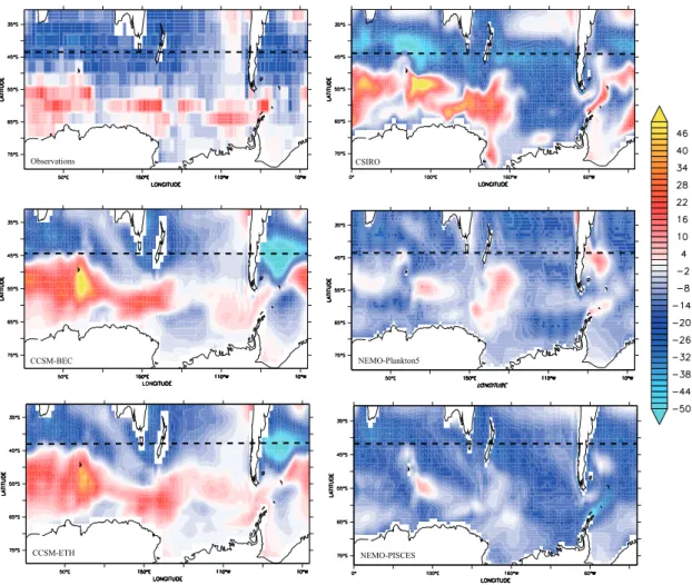
The largest median absolute deviation (MAD) in the an-nual sea–air flux is for ocean biogeochemical models (Ta-ble 3, Fig. 3). However, the small number of ocean bio-geochemical models (5) compared to atmospheric inversions (11) can result in greater MAD values for the ocean models. The spatial plots of the annual mean uptake for 1990–2009 (Fig. 4) show that all the ocean models simulate a negative sea–air flux or uptake equatorward of 50◦S. The CCSM-BEC, CCSM-ETH and CSIRO models have similar patterns of sea–air fluxes as the values derived from observations with areas of CO2flux to the atmosphere at high latitudes
(pole-ward of 50◦S) and areas of CO2 flux into the ocean to the
north of the Subantarctic front at about 50◦S; however, the fluxes to the atmosphere from these models tend to be greater than the values from observations. The CSIRO model also simulates a region of uptake in the eastern Pacific that is not apparent in the observations, although this region has few measurements to constrain the observational based estimates (Fig. 2). The NEMO-Plankton5 and NEMO-PISCES models simulate larger CO2uptake at higher latitudes compared to
observations and other models, and do not resolve the transi-tion in the flux at about 50◦S as the other models.
The different patterns of annual uptake shown in Fig. 4 results in a broad range in the cumulative annual fluxes of CO2 (Fig. 5). The cumulative fluxes from 75 to 58◦S
for the CCSM-BEC, CCSM-ETH and the CSIRO models are 0.0, +0.06 and −0.04 Pg C yr−1, respectively, and are
similar to the observation-based value of +0.05 Pg C yr−1.
The NEMO-Plankton5 and NEMO-PISCES models predict a greater sea–air CO2flux into the ocean from 75◦S to 58◦S of
−0.20 and−0.25 Pg C yr−1, respectively. A net flux of CO 2
Observations CSIRO
CCSM-BEC NEMO-Plankton5
CCSM-ETH NEMO-PISCES
Fig. 4.Spatial maps of the annual mean uptake, in g C m−2yr−1from the five ocean biogeochemical models and observations; negative
values reflect fluxes into the ocean. The dashed line represents the RECCAP boundary at 44◦S.
models. This is only partially offset in these two models by uptake in the SAZ and the resulting net annual sea–air flux at 44◦S is−0.04 Pg C yr−1(CCSM-BEC) and+0.05 Pg C yr−1 (CCSM-ETH) compared to the observation based estimate of
−0.27 Pg C yr−1.
The CSIRO model also simulates regions of net flux to the atmosphere at high latitudes (Fig. 4), but these are largely offset by other zones of uptake in the same latitudinal range, resulting in only a slight maximum in the cumulative zonally integrated flux for this model near 50◦S. A band of high CO2
uptake in the Subantarctic and subtropical waters produces a cumulative uptake to 44◦S of −0.42 Pg C yr−1 for the
CSIRO model. The cumulative uptake for both NEMO mod-els increases to 44◦S to−0.4 Pg C yr−1(NEMO-Plankton5)
and−0.8 Pg C yr−1 (NEMO-PISCES). The large deviation
in the annual uptake for the ocean biogeochemical models appears to be in part due to how the sea–air CO2 fluxes
are simulated at latitudes poleward of 58◦S (discussed in Sect. 3.1.3).
Atmospheric CO2 inversions are usually constrained not
only by the atmospheric CO2data, but also by a first guess or 1216$
1217$
1218$
STF
RECCAP
SAF PF
Observations
CCSM-BEC CSIRO
CCSM-ETH NEMO-Plankton5 NEMO-PISCES
Sea-Air CO
2
Flux (PgC/yr)
Latitude
Fig. 5.The cumulative, zonally integrated, annual mean CO2
up-take (30–75◦S integrating from the south) from the biogeochemical
ocean models and observations (dashed line) (Pg C yr−1). Overlain
are the nominal positions of the major Southern Ocean fronts and
the RECCAP boundary at 44◦S. Negative values reflect flux into
a priori flux estimate. The estimated Southern Ocean flux was not very sensitive to this prior information; across inversions prior annual fluxes were clustered around−0.35 Pg C yr−1
or −1.0 Pg C yr−1, but this clustering is not maintained in
the estimated fluxes from the inversions. This suggests that the observing network for this region may be sufficient to constrain the flux estimates. However, other differences be-tween the inversions, such as the modelling of atmospheric transport, contribute to the range in atmospheric results. For example, a transport model with vigorous mixing of higher CO2 concentration of air from the north would require a
larger Southern Ocean sink to maintain the north–south gra-dient of CO2 concentration than a transport model with
slower mixing of air from the north.
The ocean inversions do not use a priori estimates, but they may be sensitive to biases in the data based techniques used to estimate the components of the observed dissolved inorganic carbon in the ocean due to anthropogenic carbon uptake and sea–air gas exchange (e.g. Matsumoto and Gru-ber, 2005; Gerber et al., 2009, 2010). Like atmospheric in-versions, the ocean inversion is likely to be sensitive to bi-ases in model transport, particularly in the Southern Ocean, but the use of a suite of different models has been employed to help quantify this uncertainty. Although ocean CO2
in-versions have been less widely used than atmospheric CO2
inversions, this approach thus far seems to be relatively in-sensitive to the choice of inverse methodology (Gerber et al., 2010).
3.1.2 Southern Ocean, 44–58◦S
The median annual sea–air flux values for the different ap-proaches varies between−0.26 and−0.35 Pg C yr−1for the
circumpolar region from 44 to 58◦S. These values are sim-ilar to the annual uptake for the entire Southern Ocean (44–75◦S), suggesting the majority of the net uptake oc-curs in this latitude band, consistent with previous studies (Metzl et al., 2006; McNeil et al., 2007; Takahashi et al., 2009, 2012).
The contributions of the Atlantic, Indian, and Pacific Ocean sectors to the annual uptake in the 44–58◦S band are similar when all 26 models are grouped (−0.13±0.04, −0.11±0.03 and−0.11±0.04; Table 3). The ocean
biogeo-chemical models and observations do suggest that greater up-take occurs in the Pacific sector, which is not apparent in the atmospheric or ocean inversion results.
It is important to note that the flux values for all ap-proaches are associated with a large range, particularly ocean biogeochemical models (see Sect. 3.1.1) and atmospheric in-versions. This is most evident in the Indian and southeast Pa-cific oceans where ocean biogeochemical models differ in the sign of the flux (Fig. 4). For atmospheric inversions, the basin split is dependent on the spatial resolution of the inversion; inversions that solve for only 1 or 2 regions rely on their prior information to determine the basin split, while inversions that
solve for many regions may be susceptible to “overfitting” the atmospheric measurements and thereby biasing the flux estimates. This may be a particular problem for the South-ern Ocean as atmospheric CO2variations between observing
stations are very small, placing high demands on data quality and a transport model’s ability to represent that data. This is consistent with previous studies based on ocean inversions, which have shown that this approach cannot robustly sepa-rate the Indian and Pacific Ocean basins based available data (e.g. Mikaloff Fletcher et al., 2006, 2007).
3.1.3 Southern Ocean 58–75◦S
The influence of this high latitude band (40 % of the total Southern Ocean surface area) on the annual sea–air CO2flux
is small relative to the 44–58◦S region, accounting for only about 10 % of the total Southern Ocean sea–air flux (Ta-ble 3). Ocean biogeochemical models and ocean inversions indicate that this region is a small net sink of atmospheric CO2 annually (−0.04±0.09 and −0.07±0.01 Pg C yr−1),
with atmospheric inversions and observations suggesting a small net flux to the atmosphere (+0.03±0.03 and +0.04±0.02 Pg C yr−1).
Ocean biogeochemical models again show the largest range in fluxes (Table 3 and Fig. 3). This variability may be due to (i) the representation of the sea ice and associ-ated gas exchange differs across models (e.g. Rysgaard et al., 2011); and (ii) the coarse resolution of the models which pre-cludes the proper representation of potentially important fea-tures such as polynas as well as other important coastal ocean processes (Marsland et al., 2004). This part of the Southern Ocean remains one of the most poorly sampled of all ocean regions (Fig. 2; Monteiro et al., 2010) and the uncertainty in the flux estimates based on observations may be underesti-mated.
This region was regarded as a strong annual sink of atmo-spheric CO2based on summer data (Takahashi et al., 2002),
while more recent observations (Takahashi et al., 2009) have suggested that the higher latitude Southern Ocean is neutral or a weak source of atmospheric CO2over the annual mean.
These estimates are based more on open-ocean observations rather than data collected in marginal seas and coastal mar-gins of the Southern Ocean. These areas that have a high vari-ability in biological production (e.g. Sweeney et al., 2000; Hales and Takahashi, 2004) and as a consequence have been suggested to play an important role in the global carbon bud-get (Arrigo et al., 2008). Amongst the approaches in this study, only atmospheric inversions have the potential to cap-ture the integrated coastal, sea-ice and open-ocean responses in this region. That these inversions suggest that this region is not a large net sink of CO2 suggests that either: (i)
1224$
1225$
Ocean Biogeochemical Models
Atmospheric Inversions Observations Ocean Biogeochemical Models
Atmospheric Inversions Observations
Ocean Biogeochemical Models
Atmospheric Inversions Observations
Sea-Air CO
2
Flux (PgC/yr)
Sea-Air CO
2
Flux (PgC/yr)
Sea-Air CO
2
Flux (PgC/yr)
a)
b)
a)
c)
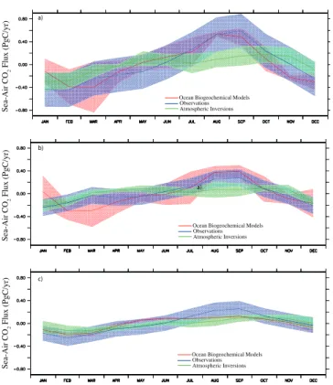
Fig. 6.Seasonal cycle anomaly of the Southern Ocean sea–air CO2
flux (Pg C yr−1) from observations, ocean biogeochemical and
at-mospheric inversions for the Southern Ocean (44–75◦S; upper), the
region 44–58◦S (middle) and the region south of 58◦S (lower). The
shaded area represents the sea-air CO2flux uncertainty associated
with each approach. Negative values reflect flux into the ocean.
3.2 Seasonal sea–air CO2fluxes
In this section we consider how the various modelling ap-proaches represent the seasonality in the sea–air CO2
ex-change compared to observations. This provides insights into the ability of ocean biogeochemical models to represent the complex interplay of physical and biological processes that drive sea–air CO2 exchange. The ability of a model to
re-produce the seasonal cycle also provides some indication of the ocean biogeochemical models ability to correctly repre-sent climate sensitive processes that could influence long-term projections of the ocean CO2uptake. The multi-model
median seasonal anomalies of sea–air CO2fluxes are shown
in Fig. 6, while the individual models and observations are shown in Fig. 7.
3.2.1 Southern Ocean 44–75◦S
Figure 6a shows the median and MAD over the entire South-ern Ocean RECCAP region. Some ocean biogeochemical models do simulate the seasonal cycle in the sea–air CO2
flux estimated from observations (Figs. 6 and 7). In sum-mer, a CO2 flux into the ocean surface (negative flux)
re-sults from the combined effects of increased surface
stratifi-1232$
1233$
Sea-Air CO
2
Flux (PgC/yr)
Sea-Air CO
2
Flux (PgC/yr)
a)
b)
Fig. 7.The seasonal sea–air CO2fluxes for the Southern Ocean
(44–75◦S) from individual ocean biogeochemical models (upper)
and individual atmospheric inverse estimates (lower). In both plots the observations are overlain (dashed black line). Negative values reflect flux into the ocean.
cation, warming, and increased biologically driven CO2
up-take. Deeper mixing and lower production, offset to some degree by surface cooling, results in a reduced flux into the ocean and potential outgassing of CO2in winter (Takahashi
et al., 2009). All approaches tend to give similar estimates in summer, but the atmospheric inversions do not capture the strong winter response evident in ocean models and esti-mated from observations.
To explore the relationship between the seasonal cycle and the annual mean uptake, we used a two-dimensional (2-D) Taylor Diagram (Fig. 8a). The annual mean uptake and tim-ing of the seasonal flux changes relative to observationally based estimates were compared for each ocean biogeochem-ical model and atmospheric inversion. The analysis provides a synthesis of the ability of all models to capture the sea-sonal and annual sea–air fluxes. In this analysis, we do not account for the uncertainty associated with observationally derived fluxes, which are associated with large uncertainties (see Sect. 2.1.1).
The x-axis in each Taylor diagram is the normalized stan-dard deviation of the seasonal cycle (σmodel/σobs); the closer
the value is to 1 (denoted as a red arc in Fig. 8) the better it reproduces the magnitude of the seasonal cycle from the ob-servations. The correlation of the model seasonal cycle with observations is shown on the arc; models or inversions with correlations of +1 (x-axis) will simulate the seasonality in
1239
1240 Fig. 8.Taylor diagram of the seasonal sea–air CO2flux assessed against the observations for ocean biogeochemical models (circles) and atmospheric inversion models (triangles). The upper panel
rep-resents the region 44–75◦S; the middle panel the region 44–58◦S;
and the lower panel the region 58–75◦S. The colours represent the
difference between the total observed annual uptake and the models (see text for a comprehensive explanation). The annual mean
differ-ences (colour bar) are in Pg C yr−1.
Ocean biogeochemical models are represented as circles, while triangles represent atmospheric inversions.
A diverse set of responses is evident in Fig. 8a. Many at-mospheric inverse and ocean biogeochemical models under-estimate the magnitude of the seasonal cycle. Several models and inversions appear to capture the magnitude and the phase of the seasonal cycle, however these models tend to strongly underestimate the magnitude of annual mean uptake (blue symbols with large negative values for the observations mi-nus model difference). Some models and inversions do a poor job at capturing the phase of the seasonal cycle, but show bet-ter agreement in the annual mean uptake. These results are particularly worrisome, given that some models are unable
to simulate even the seasonality, which is the largest scale of variability in the Southern Ocean.
The reasons behind the poor seasonality in many atmo-spheric inversions remain unclear, but two factors may con-tribute. Firstly, the observed seasonality of atmospheric CO2
in the Southern Ocean region is small, with roughly equal contributions from the seasonality of local ocean fluxes and from the transport of seasonal signals from sources and sinks in other regions. Due to the strong role of fluxes from dis-tant regions in determining the seasonal cycle in atmospheric CO2at stations that observe the Southern Ocean, errors in
the fluxes estimated from other regions or in the modelled transport of those fluxes to the high latitude southern hemi-sphere could lead to biases in the seasonal cycle. Secondly, some of the inversions that solve for smaller ocean regions (e.g. C13 CCAM law) show very different seasonality be-tween basins, suggesting some caution should be applied to those results. Possibly, the greater flexibility in those inver-sions to fit the atmospheric data makes them vulnerable to any data quality or representativeness issues as well as trans-port model errors. When inversions are solved for fewer re-gions, the inversion compromises the fit across sites effec-tively ignoring any poorly calibrated data. Conversely, in-versions that solve for only a few regions could be missing important spatial variability in the seasonal cycle, which can lead to biases in the inverse estimates (Kaminski et al., 2001). The representation of the seasonal cycle varies widely across the ocean biogeochemical models (Fig. 7). If the sum-mer warming is too strong in the upper ocean, the solubility response can dominate over the biological productivity lead-ing to a peak in the sea–air flux that is several months out of phase with observations (Fig. 8a). The net primary productiv-ity from the models (not shown) has a similar magnitude over summer. This suggests that changes in the seasonal temper-ature and mixed layer depth are likely to be more important than the differences between biological models in causing the varied responses in the ocean models. Interestingly, capturing the seasonal cycle of the Southern Ocean is not a prerequisite to reproducing the annual mean sea–air flux calculated from observations. However, the inability of the models to simu-late the observation-based seasonality in the sea–air CO2flux
does bring into question the ability of these models to realis-tically project the response of the Southern Ocean CO2flux
to climate change.
3.2.2 Southern Ocean 44–58◦S
for the Southern Ocean (Metzl et al., 2006; Takahashi et al., 2009, 2012).
The 2-D Taylor diagram for individual models (Fig. 8b) shows a diverse range of responses. Some models represent the observation-based phase and magnitude of the seasonal cycle, but do a poor job in capturing the annual uptake. Some models that do approximately represent the annual uptake can display poorer magnitude and phase of the seasonal cy-cle. While individual models may not represent both the sea-sonal cycle and annual sea–air CO2flux, taking the median
of multiple models (ensemble) agrees more favorably with the observed response.
3.2.3 Southern Ocean 58–75◦S
At high latitudes, the magnitude of the seasonal cycle in the sea–air CO2 flux is larger for fluxes derived from
observa-tions than for the ocean models and atmospheric inversions (Fig. 6c). While the annual median values (Table 3) are quite low in this region, observations indicate a relatively large summer flux into the ocean and a flux to the atmosphere in winter. Neither ocean biogeochemical models nor atmo-spheric inversions show a well-defined seasonal cycle. The atmospheric inversions show no evidence of a large summer CO2uptake (negative flux) associated with the coastal ocean
and marginal seas as suggested by Arrigo et al. (2008). The 2-D Taylor diagram showing the behaviour of the in-dividual models for this region is shown in Fig. 8c. The bio-geochemical models underestimate the seasonal cycle rela-tive to observations, but most capture the observed phase and the models tend to agree on the magnitude of the seasonal cycle, explaining the small range of the ocean biogeochem-ical models in Fig. 6c. The smaller magnitude of the sea-sonal cycle in ocean biogeochemical models may well be re-lated to the representation of the sea-ice zone as discussed in Sect. 3.1.3.
The atmospheric inversions show a diverse set of re-sponses in this region. Consistent with the median, we see that the majority of these models underestimate the seasonal cycle relative to observations. Clearly most of the models do a good job capturing the phase of the seasonal cycle but do poorly at representing the annual mean uptake. However some models, while capturing the annual mean uptake well, show very little or poor seasonality. Some inversions produce a semi-annual cycle. These results again highlight that a well-represented seasonal cycle is not a prerequisite for capturing the annual mean uptake in atmospheric inverse models well. This is also confirmed by the negligible a posteriori corre-lations between seasonal anomalies and the mean in atmo-spheric inversions (e.g. R¨odenbeck, 2005).
3.3 Longer-term variability
Understanding and quantifying interannual variability in the Southern Ocean is key to projecting the future response of
Southern Ocean sea–air fluxes. The detection of a long-term trend is difficult as observations tend to be most common in the austral summer and studies have shown that changes in sea surface temperature and net production can cause con-siderable variability in sea–air fluxes at regional scales dur-ing the summer months (Jabaud-Jan et al., 2004; Br´evi`ere et al., 2006; Borges et al., 2008; Brix et al., 2012). While a few observational studies attempt to describe the longer-term change of the carbon system, they focus on oceanicpCO2
rather than changes in sea–air CO2 fluxes (Inoue and Ishii,
2005; Lenton et al., 2012; Metzl, 2009; Midorikawa et al., 2012; Takahashi et al., 2009) or are station studies that may have local influences (Currie et al., 2009). Consequently, as we are focusing on sea–air CO2 fluxes we only use
atmo-spheric inversion and ocean biogeochemical models over the period 1990–2009, rather than observations.
3.3.1 Southern Ocean 44–75◦S
The simulated median interannual variability and associ-ated uncertainty in sea–air CO2 fluxes from ocean
bio-geochemical models and atmospheric inverse models are shown in Fig. 9. The interannual variability in the period 1990–2009 from ocean biogeochemical models and atmo-spheric inversions are of similar maximum value (+0.10 and +0.11 Pg C yr−1, respectively). This represents 20 % of the
total median sea–air flux from ocean biogeochemical models and 35 % of the median flux from atmospheric inversions. The positive and negative flux anomalies are of similar mag-nitude.
The region 44–58◦S can explain about 75 % of the inter-annual variability in the Southern Ocean sea–air CO2flux in
the atmospheric inversions (+0.07 Pg C yr−1) and ocean
bio-geochemical models (+0.08 Pg C yr−1; Fig. 9b). The
remain-ing 25 % of the interannual variability is attributable to the region 58–75◦S (Fig. 9c). These results suggest that south of 58◦S, the median interannual variability from ocean bio-geochemical models (+0.03 Pg C yr−1) and atmospheric
in-versions (+0.07 Pg C yr−1) can be as large as the net annual
sea–air CO2flux (Table 3). In this region the range in sea–air
flux for ocean biogeochemical models is lower than in the at-mospheric inverse models (consistent with Sect. 3.1.3). The large interannual variability poleward of 58◦S may be due to biogeochemical responses to changes in heat and fresh-water fluxes, wind stress and sea-ice cover. This could indi-cate that sea–air CO2fluxes in this region are more sensitive
to climate than previously believed. The sea–air CO2fluxes
in the 44–58◦S and 58–75◦S regions are correlated, which is consistent with the interannual variability being driven by large-scale Southern Ocean climate variability such as the Southern Annular Mode.
1248
1249 Fig. 9.The oceanic interannual variability in sea–air CO
2flux from
ocean biogeochemical and atmospheric inverse models in the period
1990–2009. The upper panel represents the region 44–75◦S, the
middle figure is the region 44–58◦S and the lower region 58–75◦S.
The shaded area represents the sea–air CO2flux uncertainty
associ-ated with each approach. Negative values reflect flux into the ocean.
magnitude of these variations may well reflect over sensitiv-ity to some of the atmospheric measurements. For example, the strong negative flux in 2003 may be driven by the atmo-spheric record at Jubany (58◦W, 62◦S), which has periods in 2003–2004 when the CO2 concentration is 0.7–1.0 ppm
lower than at nearby Palmer Station (64◦W, 65◦S). Conse-quently, those inversions that include this data give larger fluxes in 2003 than those that do not. It is interesting that this sensitivity occurs for inversions that span the range of flux resolution that the inversions solve for (i.e. one or many Southern Ocean regions). The positive and negative anoma-lies in 1997–1998 and 2000 are harder to attribute. Similar, though larger, anomalies are also seen for Southern Hemi-sphere land regions (Peylin et al., 2013, Fig. 6). This sug-gests that the atmospheric data may be insufficient to clearly differentiate land and ocean flux anomalies due to the usual practice of selecting atmospheric measurements to be repre-sentative of well-mixed air masses and thus removing data that has had recent contact with land.
The median of the ocean biogeochemical models shows a larger sea–air CO2flux in 2009 relative to the start of the
study period in 1990 (Fig. 9). This is expected as the CO2
gradient between the atmosphere and ocean has increased in
1256
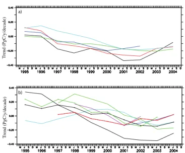
1257 Fig. 10.Trends in ocean carbon uptake in the Southern Ocean
be-tween 44–75◦S over different decadal periods (see text for
expla-nation) in units of Pg C yr−1decade−1. The upper panel shows the
trends for individual ocean biogeochemical models and the lower panel shows the trends from individual atmospheric inverse mod-els. Negative trend values reflect increasing flux into the ocean over each decadal period.
response to continuing atmospheric emissions of CO2. The
median of the atmospheric inversions shows no increase in CO2uptake over the study period. However, our confidence
in these long-term trends is low, given the magnitude of the interannual variability and the relatively short period of sim-ulations.
Figure 10a and b depict linear decadal trends computed as a function of time using a 10 yr sliding window centred on the reported year, following Lovenduski et al. (2008). The ocean biogeochemical models produce mostly negative trends, with the exception of decades centred in the mid-1990s. Atmo-spheric inversions in contrast show mostly a positive trend in the decades centred in the 1990s, and a negative trend from 2000 onwards; however, these trends are very variable both across inversions and within individual inversions, due to the large interannual variability in estimated fluxes (see Fig. 9a). Calculating the linear trend in Southern Ocean fluxes over the maximum period available from any given ocean biogeo-chemical model (18–20 yr) or inversion (13–19 yr and ex-cluding those with less than 10 yr of output) yields a me-dian and MAD trend of −0.09±0.04 Pg C yr−1decade−1
for biogeochemical models and 0±0.03 Pg C yr−1decade−1
for the inversions. This enhanced uptake in ocean biogeo-chemical models is consistent with the expected uptake of
−0.05 Pg C yr−1decade−1 of the Southern Ocean sink (Le
Qu´er´e et al., 2007), due to the increasing atmospheric CO2
large across inversions (−0.06 to 0.08 Pg C yr−1decade−1)
and previous work (Law et al., 2008) has shown that the in-version trends are likely quite sensitive to atmospheric CO2
data quality, with atmospheric CO2gradients being close to
measurement uncertainty (Stephens et al., 2013). This sug-gests that linear trends in model output over periods less than 20 yr are unlikely to provide a statistically meaningful state-ment about the very small changing rate of Southern Ocean CO2uptake. This is supported by the results of McKinley et
al. (2011) for the North Atlantic.
4 Conclusion
The Southern Ocean, despite the important role it plays in the global carbon budget remains under sampled with re-spect to surface ocean carbon. In response to these limited observations, different approaches have been used to esti-mate total net sea–air CO2exchange of the Southern Ocean
and understand different scales of variability: (i) synthesis of surface ocean observations; (ii) atmospheric inverse models; (iii) ocean inversions; and (iv) ocean biogeochemical mod-els. The goal of this study is to combine these different ap-proaches to quantify and assess how well the models rep-resent the mean and variability of sea–air CO2fluxes in the
Southern Ocean in comparison to flux estimates derived from observations. We used the recalculated sea–air CO2flux
cli-matology of Wanninkhof et al. (2013) as our observational product: five different ocean biogeochemical models driven with observed atmospheric CO2 concentrations; eleven
at-mospheric inverse models using atat-mospheric records col-lected around the Southern Ocean; and ten ocean inverse models.
Our results show that the median annual sea–air flux from all four approaches applied in the entire Southern Ocean re-gion (44–75◦S) is between−0.27 and−0.43 Pg C yr−1, with
a median value for all 26 models of−0.42±0.07 Pg C yr−1.
We see that the observation-based annual net uptake is nearly doubled to−0.47 Pg C yr−1if the boundary is shifted from
44 to 40◦S, bringing the observations and ocean biogeo-chemical model results into closer agreement. The region 44–58◦S dominates the annual flux with a median of all models of −0.35±0.09 Pg C yr−1. Ocean biogeochemical
models show the greatest mean absolute deviation in the modelled flux, which may be in part due to the RECCAP boundary at 44◦S and the proportion of the important SAZ included in this calculation. In the region south of 58◦S, both ocean biogeochemical models and ocean inversions show a small net CO2flux into the ocean (negative flux), while
at-mospheric inversions and estimates from observations show a small net flux to the atmosphere (positive flux). We see lit-tle evidence in the atmospheric inversions for the strong sink of CO2suggested by Arrigo et al. (2008) for this region.
The choice of the RECCAP boundary at 44◦S was prob-lematic in comparing our results with published values from
other studies (e.g. Metzl et al., 1999; Boutin et al., 2008; Mc-Neil et al., 2007; Barbero et al., 2011; Takahashi et al., 2012). Therefore, while we focused on the comparison between the four different techniques presented here, a more comprehen-sive analysis of individual regions needs to be undertaken in future studies. Such studies would be timely, particularly in light of recent work highlighting the heterogeneity of the anthropogenic carbon transport out of the Southern Ocean (Sallee et al., 2012).
At seasonal times scales, the fluxes estimated from obser-vations and the median of the ocean biogeochemical mod-els capture a well-defined seasonal cycle in the sea–air CO2
flux. Atmospheric inversions showed only very weak or lit-tle seasonality in all regions of the Southern Ocean. All ap-proaches tend to show enhanced flux into the ocean in the biologically productive summer period. The largest season-ality was found in the region 44–58◦S for both ocean biogeo-chemical models and based on observations. South of 58◦S, neither ocean biogeochemical models nor atmospheric inver-sions were able to capture the magnitude of the observed sea-sonal cycle. These differences between models and observa-tional estimates may reflect the model formulation and a poor understanding of the high latitude carbon cycle. None of the models were capable of simulating the magnitude and phase of seasonality and the annual mean sea–air flux at the same time in any of the regions. This raises serious concerns about projecting the future changes in Southern Ocean CO2uptake.
Interannually, ocean models and atmospheric inversions show that the variability in the Southern Ocean sea–air CO2
flux can be as large as 25 % of the annual mean. Atmospheric inversions tend to produce a larger spread in the interan-nual variability of the sea–air flux than ocean biogeochem-ical models. Both modelling approaches suggest that about 25 % of the total interannual variability can be explained by the region south of 58◦S. This implies that this variability can be as large as the net annual mean sea–air CO2 flux in
this region.
Resolving long-term trends is difficult due to the large in-terannual variability and the short time frame (1990–2009) of this study; this is particularly evident from the large spread in trends from ocean biogeochemical models and inversions. Reliable detection of Southern Ocean trends from spheric inversions requires careful assessment of the atmo-spheric CO2measurements input to inversions and their
cal-ibration over time; the provision of high quality atmospheric datasets from remote locations in the Southern Ocean is both challenging and vital. Nevertheless, in the period 1990– 2009 atmospheric inversions do suggest little change in the strength of the CO2sink broadly consistent with the results
of Le Qu´er´e et al. (2007). In contrast, ocean biogeochemical models show increasing oceanic uptake consistent with the expected increase of−0.05 Pg C yr−1decade−1(Le Qu´er´e et
al., 2007) due to increasing atmospheric CO2.
to have confidence in the projections of Southern Ocean sea– air fluxes of CO2, it is important that the models used to
un-derstand the response of the carbon cycle over the historical period not only capture the annual mean flux but also the sea-sonal cycle associated with this flux. Potentially, techniques such as water mass analysis may play an important role in helping understand the behaviour of the Southern Ocean car-bon cycle (Iudicone et al., 2011). Such models are the inte-gration of all of our knowledge and our ability to reproduce observations remains a key test of our understanding of the earth system (Falkowski et al., 2000).
Acknowledgements. A. Lenton, B. Tilbrook, R. J. Matear and
R. M. Law were funded by the Australian Climate Change Sci-ence Program and the Wealth from Oceans National Research Flag-ship. S. C. Doney acknowledges support from the National Sci-ence Foundation (OPP-0823101), T. Takahashi is supported by grants from United States NOAA (NA08OAR4320754) and Na-tional Science Foundation (ANT 06-36879). D. Baker, N. Gru-ber, M. Hoppema, N. Metzl acknowledge the support of EU FP7 project CARBOCHANGE (264879). S. C. Doney acknowledges support from the National Science Foundation (OPP-0823101). N. S. Lovenduski is grateful for support from NSF (OCE-1155240) and NOAA (NA12OAR4310058). This study is also a contribution to the international IMBER/SOLAS Projects. C. Sweeney acknowl-edges support from the United States NOAA (NA12OAR4310058) and National Science Foundation (0944761).
Atmospheric inversions were provided by F. Chevallier and P. Peylin (Laboratoire des Sciences du Climat et l’Environnement, France), K. Gurney and X. Zhang (Arizona State University, USA), A. Jacobson (Earth System Research Laboratory, NOAA, USA), R. M. Law (Commonwealth Scientific and Industrial Research Organisation, Australia), T. Maki and Y. Niwa (Meteorologi-cal Research Institute, Japan), P. Patra (Research Institute for Global Change, JAMSTEC, Japan), P. Rayner (University of Melbourne, Australia), C. R¨odenbeck (Max Planck Institute for Biogeochemistry, Germany), W. Peters (Wageningen University, the Netherlands), K. Yamada (Japan Meteorological Agency, Japan) with post-processing to a common format by P. Peylin and Z. Poussi (LSCE, France). The inversion data are available through http://transcom.lsce.ipsl.fr.
Edited by: P. Ciais
References
Arrigo, K. R., van Dijken, G., and Long, M.: Coastal Southern
Ocean: A strong anthropogenic CO2sink, Geophys. Res. Lett.,
35, L21602, doi:10.1029/2008gl035624, 2008.
Atlas, R., Hoffman, R. N., Ardizzone, J., Leidner, S. M., Jusem, J. C., Smith, D. K., and Gombos, D.: A Cross-Calibrated Multi-platform Ocean Surface Wind Velocity Product for Meteorolog-ical and Oceanographic Applications, B Am. Meteor. Soc., 92, 157–174, doi:10.1175/2010bams2946.1, 2011.
Aumont, O. and Bopp, L.: Globalizing results from ocean in situ iron fertilization studies, Global Biogeochem. Cy., 20, doi:10.029/2005GB002519, 2006.
Baker, D. F., Law, R. M., Gurney, K. R., Rayner, P., Peylin, P., Denning, A. S., Bousquet, P., Bruhwiler, L., Chen, Y. H., Ciais, P., Fung, I. Y., Heimann, M., John, J., Maki, T., Maksyutov, S., Masarie, K., Prather, M., Pak, B., Taguchi, S., and Zhu, Z.: TransCom 3 inversion intercomparison: Impact of trans-port model errors on the interannual variability of regional
CO2fluxes, 1988–2003, Global Biogeochem. Cy., 20, GB1002,
doi:10.1029/2004gb002439, 2006.
Bakker, D. C. E., Hoppema, M., Schr¨oder, M., Geibert, W., and
de Baar, H. J. W.: A rapid transition from ice covered CO2
-rich waters to a biologically mediated CO2 sink in the eastern
Weddell Gyre, Biogeosciences, 5, 1373–1386, doi:10.5194/bg-5-1373-2008, 2008.
Barbero, L., Boutin, J., Merlivat, L., Martin, N., Takahashi, T., Sutherland, S. C., and Wanninkhof, R.: Importance of water
mass formation regions for the air-sea CO2 flux estimate in
the Southern Ocean, Global Biogeochemical Cy., 25, GB1005, doi:10.1029/2010gb003818, 2011.
Borges, A. V., Tilbrook, B., Metzl, N., Lenton, A., and Delille, B.: Inter-annual variability of the carbon dioxide oceanic sink south of Tasmania, Biogeosciences, 5, 14–155, doi:10.5194/bg-5-141-2008, 2008.
Boutin, J., Merlivat, L., Henocq, C., Martin, N., and Sallee, J. B.:
Air-sea CO2flux variability in frontal regions of the Southern
Ocean from CARbon Interface OCean Atmosphere drifters, Lim-nol. Oceanogr., 53, 2062–2079, 2008.
Br´evi`ere, E., Metzl, N., Poisson, A., and Tilbrook, B.: Changes of
the oceanic CO2sink in the Eastern Indian sector of the Southern
Ocean, Tellus B, 52, 438–446, 2006.
Brix, H., Currie, K. I., and Mikaloff Fletcher, S. E.: Seasonal variability of the carbon cycle in subantarctic surface water in the South West Pacific, Global Biogeochem. Cy., 27, 200–211, doi:10.1002/gbc.20023, 2013.
Caldeira, K. and Duffy, P. B.: The role of the Southern Ocean in up-take and storage of anthropogenic carbon dioxide, Science, 287, 620–622, 2000.
Canadell, J. G., Ciais, P., Gurney, K., Le Qu´er´e, C., Piao, S., Rau-pach, M. R., and Sabine, C.: An international effort to to quantify regional carbon fluxes, EOS, 92, 81–82, 2011.
Chevallier, F., Ciais, P., Conway, T. J., Aalto, T., Anderson, B. E., Bousquet, P., Brunke, E. G., Ciattaglia, L., Esaki, Y., Frohlich, M., Gomez, A., Gomez-Pelaez, A. J., Haszpra, L., Krummel, P. B., Langenfelds, R. L., Leuenberger, M., Machida, T., Maignan, F., Matsueda, H., Morgui, J. A., Mukai, H., Nakazawa, T., Peylin, P., Ramonet, M., Rivier, L., Sawa, Y., Schmidt, M., Steele, L. P.,
Vay, S. A., Vermeulen, A. T., Wofsy, S., and Worthy, D.: CO2
sur-face fluxes at grid point scale estimated from a global 21 year re-analysis of atmospheric measurements, J. Geophys. Res.-Atmos., 115, D21307, doi:10.1029/2010jd013887, 2010.
Currie, K. I,, Reid, M., and Hunter, K. A.: Interannual vari-ability of carbon dioxide drawdown by subantarctic sur-face water near New Zealand, Biogeochemistry, 104, 23–34, doi:10.1007/s10533-009-9355-3, 2009.