www.atmos-chem-phys.net/13/8879/2013/ doi:10.5194/acp-13-8879-2013
© Author(s) 2013. CC Attribution 3.0 License.
Atmospheric
Chemistry
and Physics
Geoscientiic
Geoscientiic
Geoscientiic
Geoscientiic
The magnitude and causes of uncertainty in global model
simulations of cloud condensation nuclei
L. A. Lee1, K. J. Pringle1, C. L. Reddington1, G. W. Mann1, P. Stier2, D. V. Spracklen1, J. R. Pierce3, and K. S. Carslaw1
1Institute for Climate and Atmospheric Science, School of Earth and Environment, University of Leeds, Leeds, UK 2Department of Physics, University of Oxford, Oxford, UK
3Department of Atmospheric Science, Colorado State University, Fort Collins, Colorado, USA
Correspondence to:L. A. Lee ([email protected])
Received: 4 February 2013 – Published in Atmos. Chem. Phys. Discuss.: 8 March 2013 Revised: 14 June 2013 – Accepted: 15 July 2013 – Published: 5 September 2013
Abstract. Aerosol–cloud interaction effects are a major source of uncertainty in climate models so it is important to quantify the sources of uncertainty and thereby direct re-search efforts. However, the computational expense of global aerosol models has prevented a full statistical analysis of their outputs. Here we perform a variance-based analysis of a global 3-D aerosol microphysics model to quantify the magnitude and leading causes of parametric uncertainty in model-estimated present-day concentrations of cloud con-densation nuclei (CCN). Twenty-eight model parameters covering essentially all important aerosol processes, emis-sions and representation of aerosol size distributions were defined based on expert elicitation. An uncertainty analy-sis was then performed based on a Monte Carlo-type sam-pling of an emulator built for each model grid cell. The standard deviation around the mean CCN varies globally between about ±30 % over some marine regions to ±40– 100 % over most land areas and high latitudes, implying that aerosol processes and emissions are likely to be a signifi-cant source of uncertainty in model simulations of aerosol– cloud effects on climate. Among the most important con-tributors to CCN uncertainty are the sizes of emitted pri-mary particles, including carbonaceous combustion particles from wildfires, biomass burning and fossil fuel use, as well as sulfate particles formed on sub-grid scales. Emissions of carbonaceous combustion particles affect CCN uncertainty more than sulfur emissions. Aerosol emission-related param-eters dominate the uncertainty close to sources, while uncer-tainty in aerosol microphysical processes becomes increas-ingly important in remote regions, being dominated by
depo-sition and aerosol sulfate formation during cloud-processing. The results lead to several recommendations for research that would result in improved modelling of cloud–active aerosol on a global scale.
1 Introduction
Successive Intergovernmental Panel on Climate Change (IPCC) reports have identified aerosol direct and indirect ef-fects on climate as the largest uncertainty in the assessment of anthropogenic forcing (Schimel et al., 1996; Penner et al., 2001; Forster et al., 2007). Global aerosols can impact the climate in two distinct ways: the direct radiative effect is a re-sult of atmospheric aerosols reflecting or absorbing solar ra-diation and thereby cooling or warming the climate system. The indirect effect refers to the many ways in which aerosols interact with clouds, leading to changes in droplet concentra-tions, cloud albedo and precipitation (Lohmann and Feichter, 2005).
models are more complex than have been used in Coupled Model Intercomparison Project (CMIP) assessments (whose results feed into IPCC assessments) because they attempt to simulate the microphysical processes that determine the aerosol particle size distribution and composition on a global scale. In principle, this development in model sophistica-tion should improve model fidelity, but the increased com-plexity has led to an increase in the number of uncertain model parameters, many of which have very weak observa-tional constraints and an incomplete scientific understanding (Ghan and Schwartz, 2007). Computational constraints have also restricted the grid resolutions used for tracer transport in the models, and forced modellers to introduce simplifica-tions, such as parameterisation of the size distribution into log-normal modes or the use of a small number of bins in sectional approaches.
Assessment of multi-model diversity is the main way in which information about model uncertainty is obtained. Model intercomparison projects compare simulations of an ensemble of independent and often structurally different models over a small range of scenarios (Gates et al., 1998; Joussaume and Taylor, 1999; Meehl et al., 2000; Friedling-stein et al., 2006; Haywood et al., 2010; Kravitz et al., 2011). Many aspects of global aerosol models have been compared in this way as part of the AEROCOM project (Kinne et al., 2006; Schulz et al., 2006; Textor et al., 2006, 2007; Meehl et al., 2007; Shindell et al., 2008; Koch et al., 2009). These comparisons have provided valuable informa-tion about model diversity that underpin the assessment of aerosol impacts on climate. However, aerosol microphysics models have only recently been included in these assess-ments (Mann et al., 2013). Moreover, the multi-model en-semble approach provides limited information about how the different treatment of processes in the models drives their simulations, making it difficult to attribute the sources of model diversity. Thus, approaches based on perturbation of the parameters in a single model (often called perturbed physics ensembles, or PPEs) are a valuable approach to ex-plore uncertainties systematically in processes in a controlled way (Collins et al., 2011).
Our lack of understanding of how complex models be-have across the full parameter space has several implications for the development, evaluation and use of global aerosol– climate models. First, it means that we cannot have confi-dence in the robustness of the models; our simulations might change if a different but plausible parameter setting was used. Second, it limits what we can conclude when the model is compared against observations. Do biases represent a funda-mental weakness in the design of our model (such as missing processes) or do they simply mean that we have not evaluated or observationally calibrated our model over the full range of the parameters already in it? Third, we cannot confidently identify the model factors that most affect the uncertainty, which risks making model development an ad hoc process
rather than one driven by the desire to reduce the persistent uncertainty in aerosol forcing.
Very few studies have attempted to quantify the parametric uncertainty of a single global aerosol model because of the computational expense. The first uncertainty analysis of the aerosol indirect effect was carried out by Pan et al. (1997) using the probabilistic collocation method to produce an ap-proximation to their computer model in order to make uncer-tainty analysis feasible. Ackerley et al. (2009) studied the cli-mate responses to changes in several sulfate aerosol parame-ters as part of the Climateprediction.net project (Frame et al., 2009) with a simpler aerosol scheme than we use here. More recently, Haerter et al. (2009) studied the parametric uncer-tainty in aerosol indirect radiative forcing based on 7 cloud-related parameters with the ECHAM5 model. Lohmann and Ferrachat (2010) examined the parametric uncertainty effects on the climate in a global aerosol model by systematically varying 4 cloud parameters at specified values following a factorial design with 168 model runs. Lohmann and Fer-rachat (2010) showed a parametric uncertainty in aerosol– climate effect of 11 % when considering the uncertainty in the four cloud parameters. Another approach to understand-ing uncertainty is to use the adjoint of the model, which has been applied to cloud drop number in Karydis et al. (2012). Sensitivity analysis of cloud–aerosol interactions has been carried out by Markov chain Monte Carlo simulations us-ing an inverse modellus-ing approach in Partridge et al. (2012). The approaches require either a very large number of model simulations in a Monte Carlo-type approach (Ackerley et al., 2009) or a specific experimental design such as the factorial approach (Lohmann and Ferrachat, 2010), both of which are feasible only for a small number of parameters. However, the latest generation of global aerosol microphysics models have many tens of uncertain parameters. In order to make a real-istic assessment of the spread in model simulations, a more efficient statistical approach is required. We present a more efficient statistical approach here.
In our previous work we have demonstrated that Gaus-sian process emulators and variance-based sensitivity anal-ysis can be used to study the sensitivity of global cloud con-densation nuclei across the full uncertainty space of 8 micro-physics parameters and emissions (Lee et al., 2011, 2012). Here we extend these studies to a much more comprehensive assessment of model uncertainty covering more parameters, with the selection and range of values based on expert elici-tation. We quantify the uncertainty in cloud condensation nu-clei (CCN) due to 28 parameters, with 10 related to aerosol microphysical processes, 14 related to emissions of aerosol precursor gases and primary particles, and 4 related to the representation of the size distributions in the microphysics model. The host model physics was not perturbed.
could be applied to assess and attribute uncertainties in other key predicted quantities such as aerosol optical depth, ab-sorption or direct and indirect forcings. Our comprehensive coverage of aerosol model parameters provides the first es-sentially complete assessment of the parametric uncertainty of this key aerosol quantity. The results provide a detailed picture of the causes of model uncertainty mapped spatially and temporally across the globe for a full year. The ranked list of important parameters provides a strong steer on prior-ities for future model development and simplification.
We use the term uncertainty in this study to imply the sim-ulated range of CCN about the mean caused by an uncer-tainty range of input parameters determined by expert elic-itation. The range of uncertainty about the mean is based on a complete sampling of the aerosol parameter uncertainty space, and is presented here in terms of the standard devia-tion of a CCN probability distribudevia-tion for every grid cell of one altitude level of the model. The variance-based sensitiv-ity analysis enables the contributions to this uncertainty to be quantified. We often refer to the parameter sensitivity as the “contribution to the uncertainty”, which is justified given that we are able to calculate the absolute reduction in CCN standard deviation if a parameter were known precisely.
In Sect. 2 we introduce the global aerosol model, although this has been described in detail elsewhere. In Sect. 3 we describe the elicitation exercise, statistical approach and ex-perimental design in general terms. In Sect. 4 we describe the uncertain parameters and their physical meaning in the model. In Sect. 5 we show the validation of the emulators. The results are presented in Sect. 6 in terms of the uncertain parameters and different global regions.
2 Model description and set-up
The GLObal Model of Aerosol Processes (GLOMAP-mode) (Mann et al., 2010) is an aerosol microphysics module that simulates evolution of the size distribution and composition of aerosol particles on a global 3-D domain. The model has been used in several studies of global aerosol (Schmidt et al., 2010, 2011, 2012; Woodhouse et al., 2010, 2012; Spracklen et al., 2011b; Lee et al., 2012; Mann et al., 2012) and is a faster version of the GLOMAP-bin module that has been very widely used (e.g. Spracklen et al., 2005a,b, 2010, 2011a; Korhonen et al., 2008; Reddington et al., 2011). Both mod-els have been compared and evaluated against observations in Mann et al. (2012).
Here, the aerosol model is run within the TOMCAT global 3-D offline chemistry transport model (CTM) (Chipperfield, 2006). The same GLOMAP-mode module is also imple-mented within a general circulation model (Bellouin et al., 2013), being the aerosol component of the UK Chemistry and Aerosol (UKCA) sub-model of the Hadley Centre Global Environmental Model. In a CTM the aerosol and chemical species are transported and mixed by 3-D meteorological
fields read in from analyses, here from the European Centre for Medium-Range Weather Forecasts ERA-40 reanalyses (Uppala et al., 2005). The CTM runs here are at 2.8×2.8 de-grees with 31 vertical levels between the surface and 10 hPa. Aerosol transport is calculated on the 3-D grid every 30 min by temporally interpolating between the analyses, which are updated every 6 h. Uncoupling the aerosol from the model transport and meteorology, as we do here in the CTM, pro-vides a useful environment for our analysis, as we can ex-amine the changes in aerosol properties without the compli-cating effects of dynamical responses. If meteorology devel-oped dynamically independently in the model, we would not be able to decompose the variance into the original sources due to the extra source of variability. The dynamically evolv-ing features could be added to the statistical analyses, but that is beyond the scope of this study.
The GLOMAP-mode simulations here use the full 7-mode configuration (as in Mann et al., 2010) with one nucleation mode and soluble and insoluble modes covering the Aitken, accumulation and coarse size ranges. The modes are de-scribed by log-normal size distribution functions that are characteristic of observed particle distributions. The scheme resolves the main microphysical processes that shape the par-ticle size distribution on a global scale: emissions of primary particles and precursor gases, new particle formation, coagu-lation, gas-to-particle transfer, cloud processing and dry and wet deposition. It includes the aerosol chemical components sulfate, sea salt, black carbon (BC), organic carbon (OC) and secondary organic aerosol (SOA). The SOA is lumped with the OC component after condensation. Aerosols and precur-sor gases in GLOMAP are emitted over a few model levels: SO2 emissions from industry/power plants are emitted be-tween 100 and 300 m; volcanic SO2 and biomass burning SO2, BC and OC are emitted over a range of altitudes de-pending on the location. The model includes dust, but we have not included it among the uncertain parameters since our focus is on CCN, which we have previously shown are not strongly affected by dust particles (Manktelow et al., 2010). The important parameters and their effects in the model are described in detail in Sect. 4. The implementation of GLOMAP-mode in the CTM has been shown to compare well with ground-based and aircraft observations of aerosol mass and number (Mann et al., 2010; Schmidt et al., 2012; Spracklen et al., 2011b).
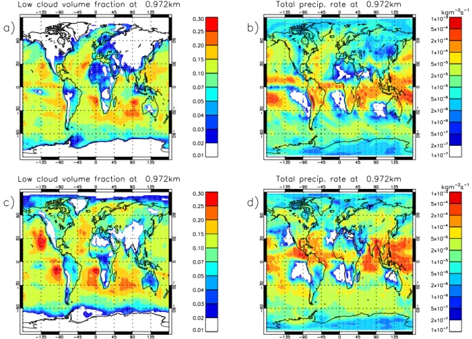
or convective are read in separately from International Satel-lite Cloud Climatology Project (ISCCP) D2 data (Rossow and Schiffer, 1999). In these clouds we assume that aerosol particles are activated and subsequently undergo “cloud pro-cessing” in which sulfate mass is added to activated aerosol due to aqueous phase oxidation of SO2(see Sect. 4 for more details). The global pattern of January and July monthly mean precipitation rate is shown in Fig. 2. This version of the model does not include aerosol wet deposition due to low-level drizzling stratiform clouds. This has been shown to be important for Arctic aerosol in our model (Browse et al., 2012) but to have a small effect on global aerosol abundance. The model was run with a set-up very similar to that described in detail by Mann et al. (2010). Additional fea-tures for these runs include anthropogenic secondary organic aerosol and replacement of an earlier binary homogeneous nucleation scheme with that of Vehkam¨aki et al. (2002) (see Sect. 4).
We present results for the year 2008. The model was spun up for three months before any parameter perturbation was applied. After this common spin-up period, the parameter perturbations were applied and a further 3-month spin-up was performed. The analysis was done on monthly mean CCN based on the following 12 months of data. At the res-olution used here, GLOMAP-mode takes about 1.5 h to run per month on 32 cores.
CCN concentrations and sensitivities are calculated at an altitude of 915 hPa (approximately 850 m a.s.l.), which is within the planetary boundary layer and at the approximate altitude of cloud base (where CCN concentrations are most relevant). We define CCN to be the number concentration of soluble particles larger than 50 nm dry diameter. CCN is a measured quantity that is usually reported at several su-persaturations of water vapour (i.e. it equates to the number of aerosol particles activated to cloud drops when a particu-lar maximum supersaturation is reached in a cloud). Super-saturation ratios in real clouds vary between less than 0.1 % in very slow updraughts to several per cent in storm clouds. Thus, no single CCN metric can provide a complete picture of the importance for cloud drop formation in all clouds. Our choice of CCN=N50 is equivalent to a supersaturation of about 0.3 % and is typical of values reached in stratocumu-lus updraught cells. If we assumed a higher supersaturation (smaller diameter of activation), then CCN would become more sensitive to processes that determine the concentration of smaller particles, and vice versa for lower supersatura-tions.
3 Statistical methods
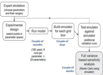
To quantify the effect of parametric uncertainty on model simulations, we apply well-established statistical methods to the global 3-D aerosol model. The overall approach is shown in Fig. 1, and consists of several distinct steps: first, expert
Fig. 1.The step-by-step approach to sensitivity analysis via emula-tion. The blue text indicates the approximate computation time.
elicitation is used to choose the uncertain model parameters and represent the uncertainty in these parameters as a proba-bility distribution. Second, statistical design is used to choose an appropriate number of model runs to explore the param-eter uncertainty space. Third, Gaussian process emulation is used to estimate model output throughout the entire parame-ter uncertainty space. A Bayesian framework is used to com-bine expert prior beliefs on parameter uncertainty and model behaviour with model runs to produce a posterior distribu-tion of model simuladistribu-tions to make global sensitivity analysis possible. Finally, a full variance-based sensitivity analysis is carried out using the emulator to quantify the sensitivity of model simulations to the parameters and their interactions conditional on the emulator and the elicited parameter proba-bility distributions. In essence, we are using emulators condi-tioned on the GLOMAP output to generate continuous model output across the parameter uncertainty space. The emulator can then be used for a Monte Carlo-type sampling of the out-put to generate sufficient data to enable a full variance-based sensitivity analysis.
3.1 Elicitation
3.1.1 General principles of elicitation
to think individually about the uncertain model parameters and to research the literature and gain as much evidence for conviction of their prior beliefs of the parameter uncertainty. Different experts should have different expertise so that the evidence is wide ranging across the different model param-eters, though all experts will have some feel for the whole model involved. The experts are then brought together, ei-ther face to face or through some online tool, and asked to discuss the model parameters to be studied and their uncer-tainty. At this stage a facilitator, most likely a statistician, is present to guide the discussion, prevent issues such as an-choring to one person’s opinion, and produce the probability distributions that result from the experts’ beliefs. Once the parameters have been chosen, the facilitator will ask the ex-perts to suggest the uncertainty range for each, such that it is highly unlikely the true value of that parameter is outside the range. The range is the most crucial part of this process since the experimental design and the emulator will be based on the ranges, whilst the shape of the uncertainty distribution of the parameters can be changed later. The shapes of the uncer-tainty distributions for the parameters are also elicited at this stage with all experts in discussion. This probability distribu-tion is not restricted to the uniform or Gaussian distribudistribu-tion. The shape of the uncertainty distribution is obtained by ask-ing the experts to split the uncertainty range into portions of different probability regions. There are various methods for obtaining the probability ranges as discussed in Oakley and O’Hagan (2010), and the experts are asked to trial them and their preferred method is used to prevent the method from impacting the results. The SHELF software is used to draw the distributions based on the experts discussions, and these are shared with experts so that feedback can be given on the resulting distribution and changes made when necessary.
One aim of expert elicitation is to remove an element of the subjectivity in such studies. As a rule, a sensitivity study fol-lows the path of an expert choosing a process to study and a few values of the associated parameter with which to run the model. In this study, we look at many more processes, so the subjectivity in choosing the processes is removed. We also ask experts to choose ranges that are beyond the normal val-ues that are used to run the model, and in fact choose ranges outside of which the parameter value is highly unlikely to fall. This approach results in a range that is wider than would normally be considered in model sensitivity studies. Further-more, the parameter ranges are elicited independently, so the uncertainty space is much larger than would normally be con-sidered because we do not let the knowledge of a particular parameter influence the others (i.e. the experts are not asked to make any judgement on the joint space of all parameters). Comparison of the results with observations will enable ex-perts to review their beliefs about model processes and pa-rameters, which is an important follow-up study.
3.1.2 Conduct of the elicitation exercise
In this study the elicitation involved six aerosol modelling experts and a statistician. The quartile method of elicitation was chosen from those in Oakley and O’Hagan (2010) fol-lowing a trial with known true answers, such as the distance from Leeds to London. The experts were given a few weeks to decide on the uncertain parameters to study and to gather evidence. The experts then discussed the uncertain parame-ters with some in a single office and others by teleconference. The range of each of the uncertain parameters was decided first and then the shape determined by cutting the range into regions of 50 % probability and then the two halves further into 50 % probability. The result of the cutting process was 4 regions all believed to contain 25 % of the probability of each parameter. Throughout the elicitation the experts were shown how the shape of the probability distributions was impacted by the decisions they made regarding the regions of proba-bility. Visualising the probability distributions proved a valu-able way of assessing the choices made by the experts. The discussions showed that some parameters were quite uncer-tain to all experts so the unceruncer-tainty ranges were quite wide whilst others could be constrained by expert knowledge and evidence. The experts chose initially 37 parameters. An ini-tial study of 5 months of the data following the same method presented here was used to eliminate 9 parameters, resulting in 28 parameters to include in the final study. The probability distributions for the 28 final parameters were agreed on by all experts after feedback. The experts were very confident in the ranges of the parameters even when the shape of the distri-bution was less certain. The details of the chosen parameters and their uncertainty distributions are given in Table 1. 3.1.3 Statistical design of the model runs
In order to build emulators of GLOMAP gridded output, 168 model runs were carried out using parameter settings sam-pled from a maximin Latin hypercube covering the uncer-tainty ranges of the 28 parameters in Table 1. Latin hyper-cube sampling splits the range in every dimension into n
initial experimental design used to build the emulator and the remaining 56 chosen using a separate Latin hypercube with the uncertainty ranges in Table 1 (Bastos and O’Hagan, 2009).
A separate emulator was built for each month over the year and for every grid box with the scalar output of CCN. At this stage no account is taken of spatial or temporal correlation. The set-up of the model runs is described in Sect. 2.
3.2 Model emulation
3.2.1 Gaussian process emulation
Gaussian process emulation (Currin et al., 1991; Haylock and O’Hagan, 1996; O’Hagan, 2006) is used to estimate model simulations at untried points throughout the space of the un-certainty of the model parameters when the computer model under investigation is too computationally expensive to be run enough times for a full Monte Carlo variance-based sen-sitivity analysis. Multivariate probability theory is used to produce a posterior probability distribution for the model simulations conditioned on model runs (training data) spread throughout the same space of uncertainty and a prior proba-bility distribution to represent prior beliefs about the model behaviour. It is important to note that the emulators are based on output of the model generated from model runs covering the parameter space; they are not an alternative version of the model physics, such as the approach used by Tang and Dob-bie (2011). First we explain the emulation method in its most general terms and then more specifically how we applied it in this study.
With the computer model (simulator) represented by the functionη, the scalar model output is defined asY =η(X), whereXis the vector of parameter values{X1, . . . , X28} in-vestigated in this study. Capital letters here represent the fact that the parameters, and therefore the model output, are un-certain. The prior probability distribution used here is the Gaussian process. This means that the prior probability dis-tribution can be specified completely by a mean function and a covariance function. The mean function is
E[η(x)|β] =h(x)β, (1)
whereh(x)is some function of xwith coefficientsβ. This represents the prior belief that the expected model output is some function of the input parametersx. The covariance function is
cov{η(x), η(x′)|σ2, δ} =σ2c(x,x′), (2) wherecis a function representing the correlation between pairs of parameter sets and depends on the distance between the pairs and the assumed smoothness of the model response to the parameters (represented byδ) whilst obeying the rules thatc(x,x)=1 and is positive semi-definite (and therefore invertible). The hyperparametersβ,σ andδare given weak
conjugate prior distributions so that they are in effect esti-mated by the training data. The training data are provided by runs of the computer model y= {y1=η(x1), . . . , yn=
η(xn)}. The choice of parameter sets used to produce the
training data is determined by some space-filling design given the ranges placed on X by the expert elicitation to gain as much information about the simulator responseη(·)
as possible over the region of interest. With the training data
y, the parametersβ, σ2 andδ are estimated. Sinceβ and
σ2are given weak prior distributions, they are calculated by maximum likelihood estimation of the training data.
ˆ
β=(HTA−1H)−1HTA−1y, (3) where
HT=(h(x1), . . . , h(xn)), (4)
A=
1 c(x1,x2)· · ·c(x1,xn)
c(x2,x1) 1 ...
..
. . ..
c(xn,x1) · · · 1
, (5)
and
ˆ σ2=y
T(A−1−A−1H(HTA−1H)−1HTA−1)y
n−q−2 , (6)
wherenis the number of training runs andq is the number of elements inβ, which depends on the prior choice ofhin Eq. (1).
The choice of Gaussian process prior means that the pos-terior probability conditioned on the training data runs will also be a Gaussian process distribution, which can be speci-fied by a mean function and a covariance function. The pos-terior Gaussian process is a result of standard conditional multivariate Gaussian theory. Therefore, the mean function is given by
m∗(x)=h(x)Tβˆ+t (x)TA−1(y−Hβ),ˆ (7) which ensures that the function passes through each of the training data points, and the posterior covariance function is
ˆ
σ2c∗(x,x′)= ˆσ2(c(x,x′)−t (x)TA−1t (x′)+(h(x)T (8)
−t (x)TA−1H)(HTA−1H)−1(h(x′)T−t (x′)TA−1H)T),
where
t (x)T=(c(x,x1), . . . , c(x,xn)) (9)
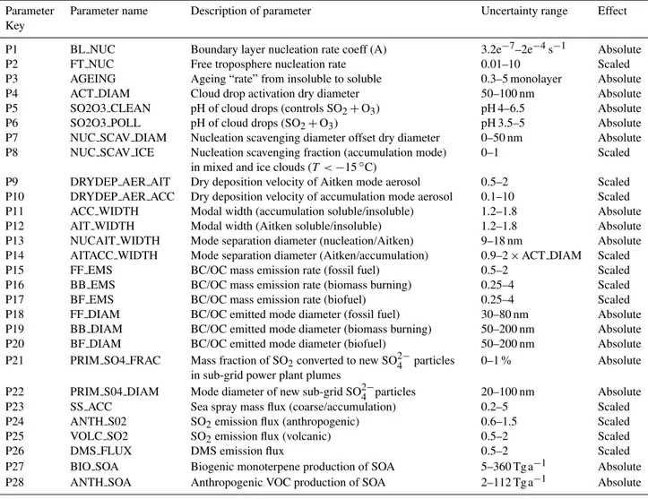
Table 1.The uncertain parameters and emissions factors
Parameter Parameter name Description of parameter Uncertainty range Effect
Key
P1 BL NUC Boundary layer nucleation rate coeff (A) 3.2e−7–2e−4s−1 Absolute
P2 FT NUC Free troposphere nucleation rate 0.01–10 Scaled
P3 AGEING Ageing “rate” from insoluble to soluble 0.3–5 monolayer Absolute
P4 ACT DIAM Cloud drop activation dry diameter 50–100 nm Absolute
P5 SO2O3 CLEAN pH of cloud drops (controls SO2+O3) pH 4–6.5 Absolute
P6 SO2O3 POLL pH of cloud drops (SO2+O3) pH 3.5–5 Absolute
P7 NUC SCAV DIAM Nucleation scavenging diameter offset dry diameter 0–50 nm Absolute
P8 NUC SCAV ICE Nucleation scavenging fraction (accumulation mode) in mixed and ice clouds (T <−15◦C)
0–1 Scaled
P9 DRYDEP AER AIT Dry deposition velocity of Aitken mode aerosol 0.5–2 Scaled
P10 DRYDEP AER ACC Dry deposition velocity of accumulation mode aerosol 0.1–10 Scaled
P11 ACC WIDTH Modal width (accumulation soluble/insoluble) 1.2–1.8 Absolute
P12 AIT WIDTH Modal width (Aitken soluble/insoluble) 1.2–1.8 Absolute
P13 NUCAIT WIDTH Mode separation diameter (nucleation/Aitken) 9–18 nm Absolute
P14 AITACC WIDTH Mode separation diameter (Aitken/accumulation) 0.9–2×ACT DIAM Scaled
P15 FF EMS BC/OC mass emission rate (fossil fuel) 0.5–2 Scaled
P16 BB EMS BC/OC mass emission rate (biomass burning) 0.25–4 Scaled
P17 BF EMS BC/OC mass emission rate (biofuel) 0.25–4 Scaled
P18 FF DIAM BC/OC emitted mode diameter (fossil fuel) 30–80 nm Absolute
P19 BB DIAM BC/OC emitted mode diameter (biomass burning) 50–200 nm Absolute
P20 BF DIAM BC/OC emitted mode diameter (biofuel) 50–200 nm Absolute
P21 PRIM SO4 FRAC Mass fraction of SO2converted to new SO24−particles in sub-grid power plant plumes
0–1 % Absolute
P22 PRIM S04 DIAM Mode diameter of new sub-grid SO24−particles 20–100 nm Absolute
P23 SS ACC Sea spray mass flux (coarse/accumulation) 0.2–5 Scaled
P24 ANTH S02 SO2emission flux (anthropogenic) 0.6–1.5 Scaled
P25 VOLC SO2 SO2emission flux (volcanic) 0.5–2 Scaled
P26 DMS FLUX DMS emission flux 0.5–2 Scaled
P27 BIO SOA Biogenic monoterpene production of SOA 5–360 Tg a−1 Absolute
P28 ANTH SOA Anthropogenic VOC production of SOA 2–112 Tg a−1 Absolute
elicited range, then the emulator can be sampled again with-out the need for more model runs. The covariance of the pos-terior distribution tells us how much uncertainty is due to us-ing emulation rather than direct simulation of the computer model. Sampling many possible functions from the posterior distribution and comparing them to the mean function will provide us with information on how robust our results are and will form part of the emulator validation in Sect. 5.
3.2.2 Emulation of GLOMAP CCN
The emulation is carried out using the R package DiceK-riging (Roustant et al., 2012). The model output y is the monthly mean CCN for each model grid cell and the model parametersx and their ranges are given in Table 1 and de-scribed in detail in Sect. 4. An emulator is built for ev-ery month and evev-ery model grid cell. In evev-ery emulator our prior beliefs assume the modelled CCN can be estimated by a simple linear regression of the parameters, and therefore
h(x)=(1, x1, . . . , x28)Tandq= 29 (p+1). The covariance structure is assumed to depend on the distance between each pair of parameter sets with a Gaussian function, and there-fore c(x,x′)=6ip==128(xi−x
′
i
δi )
2. The emulation depends on smoothness in the modelled monthly mean CCN response to each of the 28 parametersδifori=1, . . . ,28, which is
if there is reason to believe their values are known they can be used directly. In most cases there is no strong prior informa-tion on the hyperparameters so it is often necessary to use the weak priors as we do here. The assumptions of linear mean and Gaussian correlation can be changed if more information is available or when an emulator is not well validated. 3.3 Variance-based sensitivity analysis
Variance-based sensitivity analysis is used to decompose the uncertainty in the model simulations to the uncertainty in each of the model parameters (Saltelli et al., 2000). The ap-proach is able to quantify the sensitivity to each of the model parameters and their interactions (in the case of independent parameters), which cannot be done using the often applied one-at-a-time (OAT) studies. In a complex system such as the global aerosol cycle, interactions between uncertain pa-rameters are thought to be likely and the effect of these in-teractions can be studied with the variance-based sensitiv-ity analysis. The total variance of the CCN in each grid box is calculated by sampling from the emulator mean function shown in Eq. (7) given the uncertainty distributions in each of the 28 parameters obtained by the elicitation exercise.
WithYandXdefined as in Sect. 3.2.1, the emulator is used to estimate the variance (or uncertainty) around the meanY
due to the uncertainty inX,V =Var{E(Y|X)}. With inde-pendent parametersX, as we have here, the variance can be decomposed into its individual components,V =Vi+Vj+
. . .+Vm+Vi,j+. . .+Vi,j,...m, whereVp=Var{E(Y|Xp)},
andVp,q=Var{E(Y|Xp,q)}represents the variance due to
the interaction effect of parameterspandq, and so on. With an accurate emulator these estimates will be close to their true values.
In this study we use the extended-FAST method (Saltelli et al., 1999) in R package sensitivity (Pujol et al., 2008) to sample from the emulator mean function and decompose the total variance in CCN into its parametric sources. The extended-FAST method provides a more efficient sampling from the parameter uncertainty space than Monte Carlo sam-pling designed specifically for sensitivity analysis. Two mea-sures of sensitivity are calculated in the first instance. These are the main effect index and total effect index. The main effect index measures the percentage of the total variance that will be reduced if parameterpcan be learnt precisely,
Vp/V. The total effect index measures both the individual
effect and the interaction effect of each parameter with all others as a percentage of the total variance, VTp/V where VTprepresents all variance components including parameter p. The two sensitivity measures are compared to assess the sensitivity of the model output to interactions. If there are no interactions with parameterp,Vp=VTp.
4 Description of uncertain parameters and model experiments
4.1 Parameters and their meaning
As described in Sect. 3, following expert elicitation, a to-tal of 28 uncertain model parameters were identified for the perturbed parameter ensemble. The parameters relate to mi-crophysical processes, emissions of precursor gases and pri-mary particles, and the structure of the aerosol model (as-sumptions made about the representation of the size distribu-tion). The parameters are summarised in Table 1. Although some parameters (e.g. wildfire emissions) are likely to be bet-ter constrained in some regions than others, we have varied each parameter uniformly over the whole global 3-D domain, with the chosen uncertainty reflecting an upper limit for the range of their variation or uncertainty. Regional variations in the uncertainties could be studied by introducing separate parameters for each region, but we have not done this. The effect of a smaller range can be studied by adjusting the as-sumed distribution of a parameter after emulation.
4.1.1 Definition of microphysical process parameters
Nucleation rates (P1 and P2).Throughout the atmosphere we use the binary homogeneous H2SO4-H2O nucleation (BHN) rate model of Vehkam¨aki et al. (2002) scaled by a fac-tor that varies between 0.01 and 10. Zhang et al. (2010) have compared a large number of nucleation rate expressions under prescribed conditions. However, our previous studies (Spracklen et al., 2005a,b; Mann et al., 2010) show that in our model the BHN mechanism predicts total particle concentra-tions in reasonable agreement with observaconcentra-tions through the free troposphere (FT) and is therefore likely to predict a fairly realistic median rate. We assume that the rate could be a fac-tor of 100 lower but only a facfac-tor of 10 higher based on ev-idence that our model tends to overestimate particle concen-trations in the upper troposphere (UT) (Metzger et al., 2010). In the boundary layer we use a rate expression
Ageing rate (P3). Here, ageing refers to the process by which freshly emitted water-insoluble carbonaceous parti-cles (e.g. from biomass burning) become soluble following condensation of sulfuric acid and condensable organic matter. Emitted BC/OC particles enter the insoluble modes. The controlling parameter is the number of monolayers of soluble material (assumed to be SOA and H2SO4) required to convert the particles into cloud condensation nuclei, which is achieved by moving the particles from the insoluble to the soluble mode. The lower limit (0.3 monolayers) makes insoluble particles soluble within a few hours in polluted conditions, and with the upper limit (5 monolayers) this occurs on the order of days. This parameter therefore controls the particle size distribution, since particles in the soluble distribution can be wet-scavenged or undergo cloud processing, which adds sulfate mass to the particles (see parameter 8). Only particles in the soluble modes (larger than 50 nm equivalent dry diameter) are counted as CCN. This approach (developed by Wilson et al., 2001) is a simplification of a complex process in which multiple factors can affect the water solubility of the particles and their activation into cloud drops, but is widely used in global models (e.g. Stier et al., 2005; Spracklen et al., 2006).
Activation diameter (P4). The GLOMAP-mode version used here follows the approach for activation used by Spracklen et al. (2005a), whereby particles larger than a prescribed dry diameter are able to activate to cloud drops. A single value of activation diameter is used globally in a given run. In reality, the activation diameter depends on updraught speed (usually not diagnosed in models), particle composition, and the size distribution (Nenes and Seinfeld, 2003; Pringle et al., 2009), and is therefore likely to vary spatially. However, this is a computationally expensive process to simulate, with large uncertainties in the driving variables (such as unresolved cloud-scale updraughts applied over large global grid boxes). In GLOMAP, the activation diameter controls the formation of cloud drops in all low-level clouds, which we assume are non-precipitating (see Fig. 2a). Thus it mainly controls which particles undergo cloud processing (sulfate production on the particles due to oxidation of SO2 during the existence of cloud), and therefore how the size distribution is affected by clouds.
Droplet pH controlling in-cloud SO4 production from SO2+O3 (P5 and P6). The rate of the reaction SO2+O3→SO4 is controlled by the pH of cloud wa-ter (Gurciullo and Pandis, 1997; Kreidenweis et al., 2003) and has been identified as an important uncertainty in the global sulfur cycle (Faloona, 2009). We assume this reaction occurs in low-level clouds (Fig. 2a) but not in deep precipitating or frontal clouds in which the formed sulfate is rapidly removed. The pH is assumed to be the controlling parameter, which leads to a change in rate by a factor of 105for pH between 3 and 6 (Seinfeld and Pandis,
1998). One pH parameter is used for clean (lower acidity) environments (SO2<0.5 ppb) and one for polluted envi-ronments (SO2>0.5 ppb) based on measurements (Collett et al., 1994). The pH is complicated to calculate in cloud drops because it depends on kinetic and thermodynamic processes in an evolving cloud droplet distribution that are not explicitly simulated. Therefore, most models assume a fixed pH of the cloud water to control this reaction rate. Bulk models of cloud water (no droplet size resolution) underestimate the reaction rate versus droplet size-resolving models by typically a factor of 3, but sometimes much more (Hegg and Larson, 1990). This error could be larger in marine regions with large salt particles. Our parameter represents the “effective” pH of the bulk droplets, and the range takes into account the uncertainty introduced by simplifying the process.
In-cloud scavenging diameter offset (P7). In GLOMAP we assume that particles larger than DSCAV = Activa-tion diameter + diameter offset (P4 + P7) are removed in precipitation (at a rate determined by the loss rate of cloud water). The distribution of precipitation is shown in Fig. 2b. The lower limit of P7 (zero nanometres) assumes all activated particles are subject to removal during pre-cipitation. A non-zero value assumes that some activated aerosol particles escape removal based on the assumption that precipitation-sized drops are initiated by the largest cloud droplets (hence largest aerosol particles) in warm clouds. These processes can only be accurately resolved in a model that treats size-resolved cloud microphysics at very high cloud-resolving resolutions, which no global models do, so they must be parameterised in global models. We do not include the scavenging rate in warm clouds as an uncertain parameter. Previous one-at-a-time tests showed that the scavenging diameter was a much more important factor in shaping the size distribution, primarily because the scavenging lifetime in most clouds is shorter than the residence time of the aerosol in cloudy grid boxes such that the time-averaged removal becomes independent of the rate. Other models include a scavenging efficiency (fraction of particles that are accessible to scavenging in one time step). However, this is entirely equivalent to scavenging rate after multiple time steps.
Scavenging efficiency in ice-containing clouds (P8).
Fig. 2.Global low-level cloud volume fraction based on ISCCP global D2 all-cloud data (left column) and total (large-scale and convective-scale) modelled precipitation rate at∼879 hPa (right column) for January (top row) and July (bottom row).
Dry deposition of Aitken and accumulation mode particles (P9 and P10).GLOMAP calculates the wind speed and size-dependent deposition velocity due to Brownian diffusion, impaction and interception according to Slinn (1982) using resistances from Zhang et al. (2001) and three land-surface types: ocean, forest and other. In the perturbed runs, the cal-culated dry deposition velocity in each time step over each surface type is scaled for each particle size by a given factor. Taking into account the difficulty of applying dry deposition mechanisms to large global grid boxes containing unresolved inhomogeneity, we assume large uncertainties in the deposi-tion velocity of a factor of 10 for the accumuladeposi-tion mode particles (Giorgi, 1988).
4.1.2 Definition of size distribution structural parameters
Accumulation and Aitken mode widths (P11 and P12).
GLOMAP-mode uses fixed geometric widths of the log-normal size distribution modes (defined by the standard deviation of the distribution). Observations show that the width can vary in time and space (Heintzenberg et al.,
2000, 2004; Birmili et al., 2001). However, allowing for dynamically evolving mode widths adds to the complexity of the model and is therefore not widely adopted in global models. The chosen uncertainty ranges of the Aitken and accumulation mode widths were based mainly on Heintzen-berg et al. (2004) and Birmili et al. (2001). The same widths were applied for soluble and insoluble particles. Changing the mode width modifies the size distribution for particles in that mode, which in turn affects dry and wet deposition rates, and what fraction of particles are subject to cloud-processing (see P8).
in-cloud sulfate production leads to larger accumulation mode particles upon cloud evaporation. Because of this link with cloud processing, we scale this size to lie between 0.9 and 2 times the activation diameter (P4).
4.1.3 Definition of primary aerosol and precursor gas emission parameters
Fossil fuel, biofuel and biomass burning particle emission fluxes (P15, P16 and P17). The mass emission fluxes and spatial distribution of these primary particle emissions are as recommended for the harmonised emissions experi-ment in the first phase of AEROCOM (Dentener et al., 2006) using the inventories of Bond et al. (2004) and Van der Werf et al. (2003). The recommended emissions are 3.2 Tg(OA)a−1 from fossil fuel, 9.1 Tg(OA)a−1 from biofuel and 34.7 Tg(OA)a−1from wildfire/biomass burning. BC and OA fluxes are scaled by the same amounts as they are assumed to be within the same particles. The expert elicitation determined the uncertainty ranges to be a factor of 2 larger/smaller for fossil fuel combustion sources and a factor of 4 for biofuel and wildfire emissions since they are less certain (Bond et al., 2004, 2007). The uncertainty in wildfire emissions in some parts of the world (e.g. North America) may be less than a factor of 4, but this can be adjusted after the emulator is built (although we have not done that here).
Fossil fuel, biofuel and biomass burning particle emis-sion sizes (P18, P19 and P20). These parameters directly control the number of emitted particles for a given mass flux, and therefore directly influence the CCN population. The size of the emitted particles is not reported in emissions inventories, but is needed for size-resolving models, and is a major uncertainty in previous model studies of CCN (e.g. Merikanto et al., 2009; Reddington et al., 2011; Spracklen et al., 2011a). For the AEROCOM prescribed emissions experiment, Dentener et al. (2006) made recommendations for the size distribution of primary emissions based on available information in the literature. They recommended finer sizes be used for fossil fuel combustion sources than for biofuel combustion and wildfire emissions. Although more recent measurements provide some information about emitted particle number concentrations (Janh¨all et al., 2010), the particle size remains very uncertain. The size of fossil fuel combustion particles depends on the source. Biomass burning and wildfire particle size depends on burning efficiency (Janh¨all et al., 2010) amongst other parameters, but these processes are not treated in global models.
Sub-grid-scale sulfate particle production (P21 and P22).Two parameters describe the formation of particles in sub-grid-scale plumes, such as power plants and degassing volcanoes (Mather et al., 2003; Luo and Yu, 2011; Stevens et al., 2012). P21 defines the fraction of the SO2 mass that
enters the model grid square as new sulfate particles, and P22 defines the size of these particles (and hence their number concentration for fixed mass). The particles are most likely formed by nucleation and growth. Previous studies have shown this to be an important source of global CCN (Spracklen et al., 2005b; Pierce and Adams, 2006; Luo and Yu, 2011), but other studies suggest a more limited effect (Stier et al., 2006). We base our ranges on the plume-scale study of Stevens et al. (2012).
Sea spray particle mass flux (P23). We account for un-certainties in the wind-driven mass flux of sea spray particles in the size range 35 nm to 20 µm dry diameter by adjusting the baseline flux by given factors. Below 1 µm the emissions enter the accumulation mode, and at larger sizes they enter the coarse mode. This parameter conflates multiple sources of uncertainty: the function describing the wind-speed dependence of the flux, processes that are unaccounted for in the existing parameterisations (such as fetch, sea state, etc), the wind speed itself, and the effect of spatial resolution of the wind fields used by the model. The range is comparable to previous model studies (Pierce and Adams, 2006) and reflects uncertainties in the parame-terisation of measured fluxes (O’Dowd and de Leeuw, 2007).
Anthropogenic SO2emissions (P24).The baseline emissions are those from the year 2000 from Cofala et al. (2007), as used for the AEROCOM harmonised emissions experiment (Dentener et al., 2006).
Time-averaged volcanic SO2emissions (P25).The baseline emissions are as recommended by AEROCOM and are based on Andres and Kasgnoc (1998). Emissions include con-tinuously degassing volcanoes and time-averaged sporadic eruptions. We use the same uncertainty range as applied to continuously degassing emissions in Schmidt et al. (2012).
Dimethyl sulfide (DMS) emissions (P26). DMS emis-sions are controlled by the sea-water concentration of DMS and the wind-driven transfer velocity parameterisation (Nightingale et al., 2000). We conflate uncertainties in these two factors by varying the calculated sea–air transfer flux by a given factor. This approach takes into account that the absolute uncertainty in flux is likely to be higher at higher wind speeds due to the uncertainty in the flux parameterisation. Combining these two uncertainties is a reasonable approach given the lack of separate information on the global DMS sea-water concentration. The range is comparable to that predicted by different parameterisations and models (Woodhouse et al., 2010).
multi-step oxidation reactions into a single parameter that scales the VOC emissions and fixes the yield and chemical processes. In GLOMAP, SOA is produced through oxidation of transported monoterpenes (assumed to beα-pinene) by OH, NO3 and O3. The SOA yield from these reactions was assumed to be 13 % in our previous studies (Spracklen et al., 2006, 2008; Mann et al., 2010) and condenses with zero equilibrium vapour pressure (i.e. partitioned to the aerosol according to gas diffusion-limited uptake). Recent comparisons between global models and observations have suggested a global SOA source as large as 500 Tg a−1(Heald et al., 2011). Spracklen et al. (2011b) used a comparison between the model and organic aerosol observed by the aerosol mass spectrometer to suggest a global SOA source of 50–360 Tg a−1. There may be spatial variations in the uncertainty in yield that are different to the spatial uncer-tainty in emissions, but there is not enough understanding to constrain these two uncertainties separately. There are also uncertainties in the volatility of different compounds (Spracklen et al., 2011b) that we do not account for here.
Anthropogenic SOA production (P28). Uncertainty in anthropogenic SOA is treated in a similar way to biogenic SOA, by conflating the uncertainty in emissions and yield into a single emission uncertainty. For emissions of anthro-pogenic VOCs (VOC A), we used the same approach as in Spracklen et al. (2011b) by scaling gridded CO emissions from the IPCC. In Spracklen et al. (2011b) SRES CO emissions from anthropogenic activity (470.5 Tg(CO)a−1) were scaled using VOC/CO mass ratios of 0.29 g/g so as to reproduce the global sum of VOC emissions from the Emissions Database for Atmospheric Research (EDGAR) for anthropogenic sources (127 Tg(VOC)a−1). Here we vary these emissions to produce total anthropogenic SOA that lies between 2 and 112 Tg a−1. We included the reaction of VOC A with OH.
5 Validation of the emulator
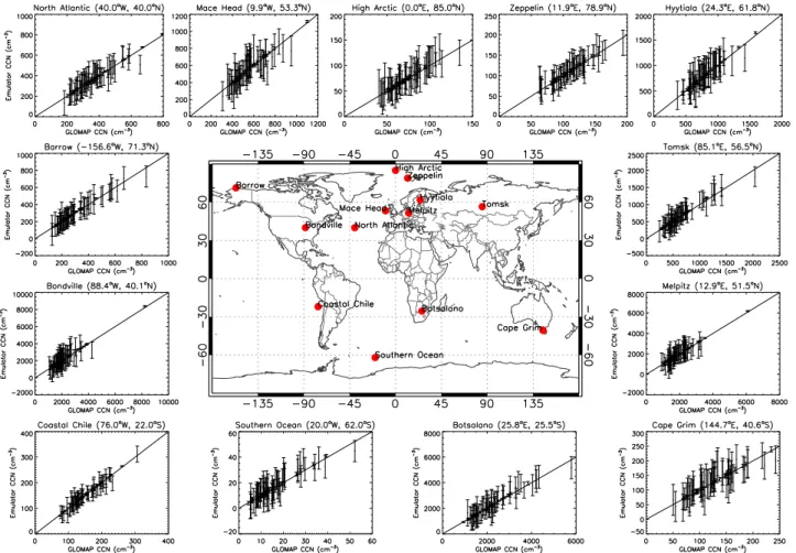
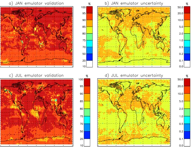
Figures 3 and 4 show the validation of the emulator. Scatter plots of the emulator estimates versus the GLOMAP vali-dation runs at various grid box locations are shown in Fig. 3, with the 95 % confidence intervals around the emulator mean calculated using Eq. (9). Figure 4a and c show maps of the January and July global emulator validation in terms of the percentage of GLOMAP validation runs that lie within the 95 % confidence interval of the emulator estimate. In most grid cells over 90 % of the GLOMAP validation simulations lie within the 95 % confidence interval of the emulator. Note that the mean emulator estimate is used for the Monte Carlo-type sampling (Sect. 3.3), and Fig. 3 shows that the emulator mean CCN is very close to the GLOMAP simulation, shown by the 1:1 line.
If the emulator is to be useful, then the uncertainty needs to be less than the parametric uncertainty that we are aiming to quantify. The emulator uncertainty is compared to the para-metric uncertainty in Fig. 4b and d. The emulator uncertainty was calculated as the standard deviation around the mean of 10 000 Gaussian process functions sampled from the emula-tor (Eqs. 7 and 9). Figure 4b and d show that the emulaemula-tor uncertainty is less than 10 % of the parametric uncertainty.
The validity of the emulator can also be assessed subjec-tively by examining the maps of parametric uncertainty (next section). The CCN and sensitivity maps are produced from an analysis of 8192 independent emulators (one for each grid cell), and yet we find that the spatial patterns can be readily understood in terms of the driving processes, implying that the emulator mean is not dominated by its uncertainty in the different grid boxes. There may be grid boxes that are less well emulated, but for the purpose of our global analysis the emulators here are considered valid.
6 Results
6.1 Metrics of uncertainty
We describe the results in terms of three measures of uncer-tainty.
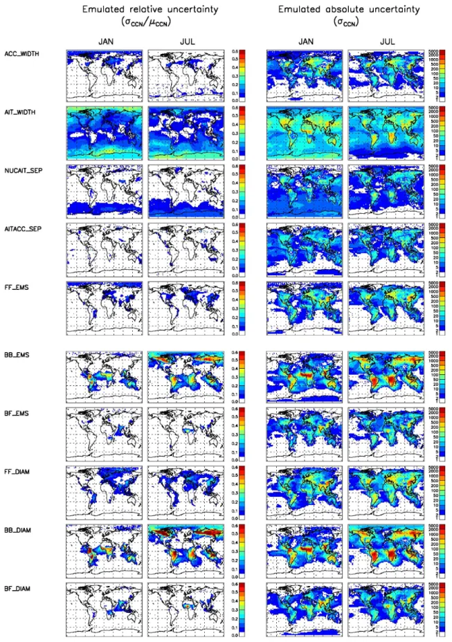
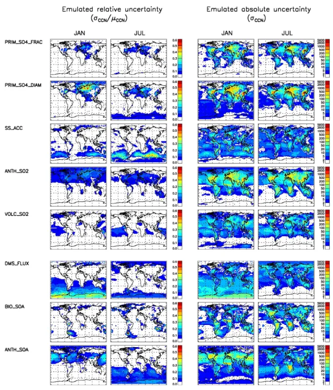
The standard deviationof the CCN probability distribu-tion in each grid cell provides a direct measure of the abso-lute uncertainty in CCN caused by the uncertain parameters. It is calculated as the square root of the total variance due to the uncertainty in the 28 parameters (see Sect. 3.3). Figure 5 shows January and July maps of emulator-estimated CCN and the standard deviation, while Fig. 6 gives some exam-ples of the probability distribution of CCN for selected loca-tions, from which the standard deviation was calculated. We also carry out a variance-based sensitivity analysis to quan-tify the contribution of each parameterito the variance in the modelled CCN. These parameter effect variances can also be mapped (Lee et al., 2012). Here we show maps of the
σCCNuncertainty in CCN (σCCN,i=
p
VCCN,i for parameter
i whereV is the variance). TheσCCN,i value is the square
root of the main effect index times the total variance for pa-rameteri (see Sect. 3.3). TheσCCN2 ,i’s cannot be added to obtain the total uncertainty in Fig. 5 unless there is zero in-teraction between the parameters.
The coefficient of variation, or relative uncertainty, is the standard deviation divided by the emulator mean CCN (σCCN,i/µCCN). This is shown also in Fig. 7. Relative
Fig. 3.Grid box validation of emulator-predicted CCN. CCN concentrations predicted by the emulator are compared against CCN from 84 additional GLOMAP model simulations in 13 model grid boxes on the 915 hPa model level. The emulator uncertainty is shown as the 95 % confidence interval around the emulator estimate calculated from Eqs. (7) and (9).
climate than the absolute uncertainty. For other quantities, like black carbon mass concentrations, the direct aerosol ef-fect depends approximately linearly on column mass, so the absolute uncertainty in BC would be more relevant.
Thefraction of varianceexplained by a parameter is the reduction in variance that would be obtained if a particular parameter were known precisely. A parameter with a large contribution to variance may have its effect in a region with overall low variance. It is therefore a measure of local “re-search priority” (improved knowledge of highly ranked pa-rameters would lead to a greater reduction in uncertainty in CCN) but not directly relevant to the impact on clouds and climate. Thus, information on CCN relative uncertainty and fraction of variance can be used together to estimate the ef-fect of an uncertain parameter on climate and to identify the most important parameter in terms of reducing the uncer-tainty in the model.
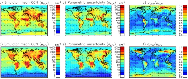
6.2 Magnitude of uncertainty in global CCN
Figure 5 shows that the standard deviation correlates well with mean CCN concentrations, but this is not the case for the relative uncertainty. In general, the relative uncertainty is lower at low latitudes than at high latitudes, although there are exceptions in the biomass burning regions. It varies be-tween a minimum of about±30 % in many clean marine re-gions and about±40–100 % over land areas and at high lati-tudes. The peakσCCNreaches 100 % over the January Arctic and July Antarctic. There is a clear seasonal cycle in rela-tive uncertainty in parts of the Northern Hemisphere (NH). For example, wintertime NH marine regions reach about 30– 50 % but generally less than 30 % in summer. Peaks in un-certainty at summer high latitude continental locations are associated with large uncertainties in wildfires, as we show below.
Fig. 4.Global validation of emulator-predicted CCN. CCN concentrations predicted by the emulator are compared against CCN from 84 additional GLOMAP model simulations for every model grid box on the 915 hPa model level. The fraction of GLOMAP simulations lying within the emulator 95 % confidence interval for every grid box is shown for(a)January and(c)July. In(b)and(d)the emulator uncertainty is shown as the standard deviation around the mean due to the emulator uncertainty (σemulator) divided by the standard deviation due to the uncertain parameters (σCCN, shown in Fig. 5). Thus, everywhere, the emulator uncertainty is less than 10 % of the parametric uncertainty.
et al., 2011a). In that study theσCCN range in modelled mi-nus observed CCN was at least 100 %. Some of this model– observation scatter may be due to poor collocation of the modelled and observed concentrations.
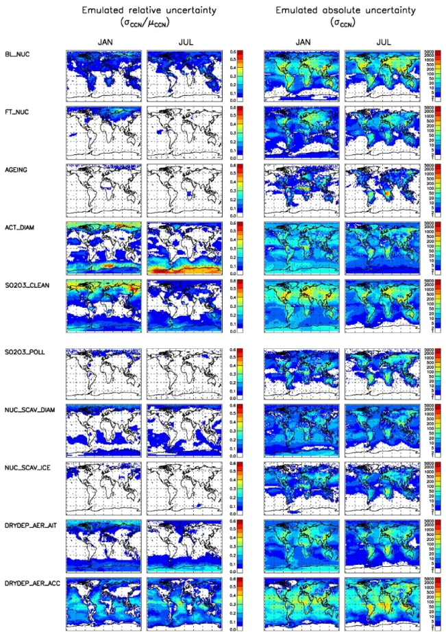
6.3 Factors controlling uncertainty in CCN
The variance-based sensitivity analysis was carried out on each model grid box separately. Figure 7 shows the global distribution of the absolute and relative CCN uncertainty, and Fig. 8 shows a global summary of the ranked relative uncer-tainties. The ranked bar charts were calculated by globally averaging σCCN,i/µCCN over all grid boxes at 915 hPa, in-cluding a weighting for grid box area. We also stratify the global data into clean/polluted according to the black carbon concentration (clean <50 ng m−3, polluted >100 ng m−3) (Fig. 8c) and by weighting σCCN,i/µCCN by cloud frac-tion based on the Internafrac-tional Satellite Cloud Climatology Project (ISCCP) global D2 all-cloud data (Rossow and
Schif-fer, 1999) (Fig. 8d). The cloud fraction is shown in Fig. 2a. Figure 8a and b also distinguish parameters according to whether they describe processes, emissions, model struc-tures, or a combination of processes and emissions (the two SOA-related parameters). These global mean bar charts sum-marise the global importance of parameters.
Fig. 5.Global fields of CCN concentration and associated uncertainty on the 915 hPa model level. Left column (aandd), mean CCN (µCCN) predicted by the emulators for January and July. Middle column (bande), uncertainty in CCN (defined as the emulator standard deviation σCCNdue to the uncertain parameters). Right column (candf), coefficient of variation (σCCN/µCCNin each grid box).
when it is included in the model, the aerosol is insensitive to the choice of rate within the range we have tested: the pro-cess could possibly be simplified but not eliminated. Third, the contribution of a parameter to aerosol variance does not imply a positive association. For example, increases in bio-genic SOA could lead to decreases in CCN due to increases in aerosol surface area and suppression of nucleation.
Below we describe the factors controlling uncertainty in CCN first by parameter and then by region and season.
6.3.1 Uncertainty due to microphysical processes
Nucleation rates (P1 and P2).The peak effect of uncertainty in the rate of boundary layer nucleation on the CCN standard deviation is about 200–500 cm−3, or a maximum CCN relative uncertainty of 20 % in any region, although we show in Section 6.3.6 that the peak contribution can locally reach 40 % in some months. The fraction of variance is also generally less than 40 %, highly localised over remote parts of summertime Canada, the European boreal forest, the Arctic, South Africa and parts of Asia. The FT nucleation rate is a process of high importance to CCN (Merikanto et al., 2009) but relatively insensitive to the rate. The greatest contribution to the standard deviation is mostly over land areas, reaching aσCCNof 100–200 cm−3and a peak relative uncertainty of about 25 % at high latitudes, but generally less than 10 %. The regions where the FT nucleation rate is most important do not coincide with regions where it makes the greatest contribution to nucleated CCN – over subtropical marine regions. Over clean regions the production of CCN is mainly through slow coagulation through the dry FT, making the CCN insensitive to the initial nucleation rate in
the UT. Over polluted regions with higher vapour supply, there is more condensational growth of the particles, and a larger fraction survive to CCN, making the CCN in the BL more sensitive.
Ageing (P3). Ageing makes a localised contribution to variance over biomass burning and other BC source regions, of up to 2000 cm−3 σCCN uncertainty in regions with very high CCN of 5000 cm−3. However, the relative uncertainty is typically less than 10 % in these regions, and the fractional contribution to variance is everywhere less than 5 %. This low sensitivity is partly because of the much larger effect of uncertainty in the mass flux and size of the emitted particles (see below) and partly because ageing timescales are only important up to the point at which most particles have aged. Ageing is therefore a relatively unimportant source of uncertainty in these regions.
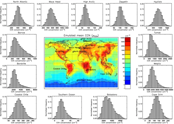
Fig. 6.The frequency distribution of CCN concentrations across the 28-dimensional parameter uncertainty space simulated from the emu-lators. Distributions are shown for July for 13 model grid boxes corresponding to the locations in Sect. 6.3.6 and Fig. 9. The map of mean CCN is the same as in Fig. 5. In some cases the CCN concentration is negative when in reality it will be truncated at zero meaning that the uncertainty in some places will be slightly overestimated. Since the negative CCN is confined to a small region of the parameter uncertainty space, the sensitivity analysis results will be robust to the negative values. Emulator calibration is not part of this study, but the first regions of parameter space to be removed will be those that give negative values.
Droplet pH controlling in-cloud SO4 production (P5
and P6). The droplet pH controlling the rate of reaction SO2+O3=SO4is an important parameter controlling much of mid-northern latitude CCN uncertainty in air affected by long-range transport of pollution in all seasons except sum-mer. Figure 8a shows that the droplet pH is the third-most important parameter controlling CCN uncertainty in winter. It accounts for up to 70–80 % of variance over large areas of Alaska and Asia, and generally 20–30 % of Arctic CCN in winter. The absolute impact on CCN peaks over polluted regions, reaching aσCCNuncertainty over E. US and Europe and China of 500 cm−3, but the relative uncertainty peaks at about 30–40 % in the Arctic winter, making it one of the most important parameters there. This pattern is consistent with the seasonal importance of the chemical reaction SO2+O3, while in summer SO2oxidation in cloud water is controlled by H2O2. Under polluted conditions (pH between
3.5 and 5, controlled by P6) the uncertainty is relatively unimportant compared to cleaner conditions in which the pH lies between 4 and 6.5 (P5).
Fig. 7.Continued.
greatest over marine regions and the wintertime Arctic, but is everywhere less than about 20 %. Thus, it appears that, at the altitude of cloud base, CCN concentrations are relatively insensitive to in-cloud nucleation scavenging assumptions, other than assuming all activated particles are scavenged. However, as we showed in Lee et al. (2012) the scavenging diameter becomes a dominant parameter throughout most of the FT.
10–30 % of BC variance in winter.
Dry deposition of Aitken and accumulation mode par-ticles (P9 and P10). The effect of dry deposition on the standard deviation follows the changes in aerosol abundance, consistent with it being a first-order loss process. The dry deposition of accumulation mode particles is more important for CCN than Aitken mode, even though the rate is lower (primarily because CCN reside mostly in the accumulation mode). It is largest over land and on continental outflow regions. The map of relative uncertainty is quite different, with a 10–30 % effect over almost all marine regions and a negligible contribution over almost all land areas. The fractional contribution to variance reaches∼30 % in regions where few other factors are important, such as in the tropics. Although dry deposition of accumulation mode particles is quite slow (particle lifetimes of up to several days), it is the dominant (or even sole) loss process of accumulation mode particles close to the surface in many regions. Unlike other processes and emissions, it is a first-order loss process that occurs continuously and everywhere. Thus, globally averaged, it is an important factor in the relative uncertainty in CCN in the boundary layer. We also note the lack of precipitation.
6.3.2 Uncertainty due to size distribution parameters
Accumulation and Aitken mode widths (P11 and P12).The accumulation mode width has an effect over polluted NH regions, reaching a maximum relative uncertainty of 10 % in the wintertime Arctic. The width of the Aitken mode has a much more widespread absolute effect over NH polluted regions and hotspots in biomass burning areas. The relative uncertainty in CCN reaches 30 % in the wintertime Arctic and 40 % over the Antarctic and parts of the Southern Ocean. As a fraction of total variance, it accounts for 10–30 % over large regions of the ocean including the Arctic. Thus the Aitken mode width is a structural parameter of high impor-tance for reducing uncertainty in predicted CCN of 50 nm dry diameter. Figure 8c and d show that the Aitken mode width is the second-most important uncertain parameter for CCN in clean and cloudy regions. The Aitken mode width is more important for CCN uncertainty than the accumulation mode width because almost all accumulation mode particles are counted as CCN, while the fraction of Aitken mode that is counted depends on how the distribution extends beyond the assumed CCN size of 50 nm dry diameter. This is the only parameter that has a significantly different impact on CCN uncertainty in cloudy versus non-cloudy regions.
Mode separation diameters (P13 and P14). The effect of the nucleation–Aitken separation diameter is restricted almost entirely to high southern latitudes of the Southern Ocean and Antarctica, accounting for a maximum of about 5 % of variance and a relative uncertainty of less than 10 %.
The Aitken–accumulation mode separation diameter has an absolute effect mainly over polluted regions. The fractional effect is restricted to a few small hotspots, reaching 8 % of variance.
6.3.3 Uncertainty due primary aerosol and precursor gas emissions
Fossil fuel particle mass flux and diameter (P15 and P18).
Fossil fuel particle emissions have a highly localised generally less than 10 % effect on σCCN/µCCN over the main source regions, especially China. The size of the emitted particles is much more important for uncertainty in CCN than the mass emission flux. The size parameter has a maximum effect on relative uncertainty of 30 % over polluted regions and accounts for 50–60 % of the variance (σCCNof 500–1000 cm−3), but typically less than 10 % over the US, where sulfate parameters are more important. The fossil fuel diameter is the fourth-most important for CCN uncertainty in polluted regions.
Biomass burning particle mass flux and diameter (P16 and P19). The importance of the biomass burning mass flux follows the seasonality of the emissions and reaches 40 % of variance over large regions mostly immediately over the sources (Amazon, Africa, northern and western US and boreal regions), which equates to a σCCN uncertainty greater than 1000 cm−3and relative uncertainty of 40–50 %. The size of the emitted particles is more important than the mass flux and causes aσCCN/µCCNuncertainty of over 60 % in source regions and 50 % over the summertime Arctic. Locally it is by far the dominant parameter and accounts for up to 80 % of the variance over source regions and up to 40– 50 % over large regions of the remote Arctic in summer. The importance of the emission parameters is strongly located over the emission regions, with very little extension over the downwind ocean regions. In these regions dry deposition becomes important (see below). The reliability of this result will depend on the realism of vertical mixing of plumes in the model, and could be tested against observations. The biomass diameter is globally ranked number three in July, but number one in polluted regions.
Biofuel particle mass flux and diameter (P17 and P20).