www.atmos-chem-phys.net/12/6845/2012/ doi:10.5194/acp-12-6845-2012
© Author(s) 2012. CC Attribution 3.0 License.
Chemistry
and Physics
Determinants and predictability of global wildfire emissions
W. Knorr1, V. Lehsten1, and A. Arneth2,1
1Physical Geography and Ecosystem Analysis, Lund University, S¨olvegatan 12, 22362 Lund, Sweden 2KIT/IMK-IFU, Kreuzeckbahnstr. 19, 82467 Garmisch-Partenkirchen, Germany
Correspondence to:W. Knorr ([email protected])
Received: 2 December 2011 – Published in Atmos. Chem. Phys. Discuss.: 6 February 2012 Revised: 8 June 2012 – Accepted: 23 July 2012 – Published: 1 August 2012
Abstract.Biomass burning is one of the largest sources of at-mospheric trace gases and aerosols globally. These emissions have a major impact on the radiative balance of the atmo-sphere and on air quality, and are thus of significant scientific and societal interest. Several datasets have been developed that quantify those emissions on a global grid and offered to the atmospheric modelling community. However, no study has yet attempted to systematically quantify the dependence of the inferred pyrogenic emissions on underlying assump-tions and input data. Such a sensitivity study is needed for understanding how well we can currently model those emis-sions and what the factors are that contribute to uncertainties in those emission estimates.
Here, we combine various satellite-derived burned area products, a terrestrial ecosystem model to simulate fuel loads and the effect of fire on ecosystem dynamics, a model of fuel combustion, and various emission models that relate com-busted biomass to the emission of various trace gases and aerosols. We carry out simulations with varying parameters for combustion completeness and fuel decomposition rates within published estimates, four different emissions mod-els and three different global burned-area products. We find that variations in combustion completeness and simulated fuel loads have the largest impact on simulated global emis-sions for most species, except for some with highly uncer-tain emission factors. Variation in burned-area estimates also contribute considerably to emission uncertainties. We con-clude that global models urgently need more field-based data for better parameterisation of combustion completeness and validation of simulated fuel loads, and that further valida-tion and improvement of burned area informavalida-tion is neces-sary for accurately modelling global wildfire emissions. The results are important for chemical transport modelling stud-ies, and for simulations of biomass burning impacts on the atmosphere under future climate change scenarios.
1 Introduction
Wildland fires have an important impact on the atmospheric load of trace gases and aerosols, on air pollution, and climate (Seiler and Crutzen, 1980; Langmann et al., 2009). Fire has also been recognized as an important agent in the workings of the Earth system, because it is an intrinsic feature of most terrestrial ecosystems and responds both to climate change and human intervention (Bowman et al., 2009; Arneth et al., 2010). In response, comprehensive datasets have been de-veloped that characterize the extent of fires globally from satellite data (Gr´egoire et al., 2003; Simon et al., 2004; Roy et al., 2005; Mouillot and Field, 2005; Giglio et al., 2006, 2010; Tansey et al., 2008), as well as the chemical emissions from those fires (Schultz, 2002; Duncan et al., 2003; Hoelze-mann et al., 2004; van der Werf et al., 2006, 2010; Schultz et al., 2008; Mieville et al., 2010). Those data sets can be used to study the effects of wildfires on air pollution and cli-mate (Langmann et al., 2009), while others that differenti-ate between types of biomass burning sources are also useful for better characterizing the role of fires in the Earth system (e.g. van der Werf et al., 2010).
data still shows large discrepancies (Thonicke et al., 2001, 2010; Prentice et al., 2011).
Before including fire in comprehensive Earth system mod-els, it is necessary to assess our current ability to model the different steps necessary for computing chemical emissions from wildfires. These steps include characterization of area burned, quantification of the amount of biomass combusted per area burned, and amount of chemical species emitted per unit amount of biomass combusted. Only if we better under-stand how sensitive simulated emissions are to uncertainties in each of these steps can we, for example, judge how well we need to reproduce burned area by prognostic models, or how accurately we need to simulate fuel loads and combus-tion factors.
The commonly used approach to compute pyrogenic emis-sions is to combine information on fire occurrence and extent with information on available fuel, combustion completeness (i.e. fraction of fuel combusted in a fire), and conversion rates of combusted fuel to the emitted amounts of various trace gases (Seiler and Crutzen, 1980). Relevant observations that cover the entire earth are available only from satellite remote sensing. Such products include fire occurrence counts de-tected by radiant emissions from fires in the middle infrared (Matson and Dozier, 1981), or the detection of burn scars by analysing bidirectional surface reflectance (Govaerts et al., 2002; Roy et al., 2005).
Fuel load is more difficult to derive from remotely sensed information. Studies using radar or LIDAR are promising but rely on locally trained image classification (e.g. Mutlu et al., 2008), or can only sense fuel contained in standing struc-tures (Saatchi et al., 2007). To the knowledge of the authors there is no global product of fuel load available that is based on these techniques. Therefore, ecosystem models are often used to model fuel load (e.g. van der Werf et al., 2010), which depends not only on plant type distribution and climate, but also on the effect of the fires itself (Thonicke et al., 2010). Observations of the combustion process are even more dif-ficult to obtain from the field, with the closest being obser-vations of radiant energy from satellites, which can be used for estimating the total amount of energy generated by the fire (Wooster et al., 2005). Since this technique is still under development (Boschetti and Roy, 2009; Ellicott et al., 2009), the fraction of fuel combusted in a fire is usually an assumed or modelled value (Ito and Penner, 2004; Arora and Boer, 2005; Wiedinmyer et al., 2006; Thonicke et al., 2010).
The provision of emission fields for biomass burning based on global models and satellite observations is al-ready a useful and important step for the atmospheric mod-elling community. It allows assessing how important pyro-genic emissions are for the total atmospheric trace gas or aerosol load, and their contribution to interannual variations and episodes (Langmann et al., 2010). Modelled trace gas fields can be compared to those trace gases that are easy to observe, such as carbon monoxide, to evaluate chemical transport and emissions modelling together (Langenfelds et
al., 2002; Kopacz et al., 2010). However, the variety of ap-proaches to compute emissions leads one to suspect that the use of different observations and models will yield varying emission fields, and any comparison between modelled and observed atmospheric trace gases or aerosol loads needs to take into account that a whole range of possible emission fields exists, some of which may lead to better and some to worse agreement with atmospheric observations. Only if we narrow down uncertainties for simulating current emissions can we hope to develop reliable models for assessing the im-pact of climate change on these emissions.
In this study, we therefore pose the following question: how sensitive are simulations of chemical emissions from wildfires to varying assumptions and data currently available in the published literature?
2 Methods
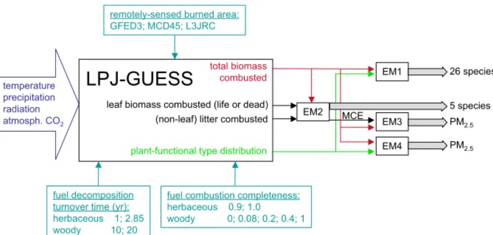
We combine remotely sensed burned area with modelled fuel loads from the Lund-Potsdam-Jena General Ecosystem Sim-ulator (LPJ-GUESS) (Smith et al., 2001). The flux of car-bon from fire to the atmosphere computed by LPJ-GUESS is subsequently fed into a set of separate models to com-pute emissions of various trace gases (Fig. 1). We explore the sensitivity of modelled chemical emissions to the differ-ent algorithms and parameterizations for emissions and fuel combustion, as well as remotely sensed burned area. We also propagate reported uncertainties in emission factors to the fi-nal results. Fifi-nally, we compare the sensitivity of modelled emissions to uncertainties in emission factors, to the choice of emission model and burned area data set, and uncertain-ties regarding the parameterisations of fuel combustion and turnover.
The purpose of this work is to explore the sensitivity of modelled wildfire emissions to various key inputs and param-eterizations, where these imputs are varied within reasonable bounds based on published data and estimates. This method mainly serves the purpose of pointing out areas that need fur-ther refinement or validation. The modelling framework with its associated flow of information is illustrated in Fig. 1.
We deliberately choose a simple approach to fire mod-elling, instead of a fully prognostic fire model, in order to make the chain of factors entering the sensitivity study as transparent as possible. Instead of computing burned area and assessing how different parameterisations of the burned-area model affect the results, we use a variety of burned burned-area products as input.
2.1 Ecosystem and fuel combustion model
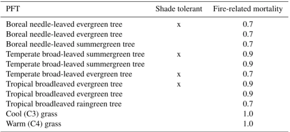
Table 1.Plant functional types and fire-related mortality used with LPJ-GUESS.
PFT Shade tolerant Fire-related mortality
Boreal needle-leaved evergreen tree x 0.7
Boreal needle-leaved evergreen tree 0.7
Boreal needle-leaved summergreen tree 0.7
Temperate broad-leaved summergreen tree x 0.9
Temperate broad-leaved summergreen tree 0.9
Temperate broad-leaved evergreen tree x 0.7
Tropical broadleaved evergreen tree x 0.9
Tropical broadleaved evergreen tree 0.9
Tropical broadleaved raingreen tree 0.7
Cool (C3) grass 1.0
Warm (C4) grass 1.0
exchanges are computed on a daily time step, while establish-ment, growth, allocation, mortality by general disturbance and competition are simulated with a yearly time step. We use the global version of LPJ-GUESS with 13 plant func-tional types (PFTs), comprising nine tree and two grass PFTs (see Table 1). LPJ-GUESS is used in cohort mode, where groups of individuals of similar age and size, or “cohorts” are represented by a single individual. We run LPJ-GUESS with five patches per grid cell, and a stochastic general patch de-stroying disturbance with an average return interval of 100 yr. This general, unspecified disturbance represents other catas-trophic events than fire (e.g. windfall or insect outbreaks) to prevent unrealistically high stand ages where no fires occur (Smith et al., 2001).
As input data we use the gridded Climate Research Unit TS3.1 monthly observations of diurnal mean temperature, precipitation and percent of potential (full sunshine) insola-tion for the period 1901 to 2009 (Mitchell and Jones, 2005; Jones and Harris, 2011), following a spin-up procedure de-scribed by Sitch et al. (2003). Annual atmospheric CO2 con-centration is derived from ice-core data (Etheridge et al., 1996) and atmospheric measurements obtained at Maona Loa, Hawaii (Keeling et al., 1995). The model is run on a global quasi-1-degree equal-area grid with 10 525 non-glaciated land grid points. The grid has a resolution of 1 de-gree latitude by 1 dede-gree longitude at the equator, with the same spacing along lines of equal latitude when away from the equator.
In variation to the standard LPJ-GUESS model, fire-related mortality is computed on a monthly time step by burning each patch with a probability equal to the observed burned fraction of the corresponding grid cell. If a patch burns, a random fraction of the cohorts representing woody PFTs is killed, where the average number of cohorts killed equals the PFT-dependent fire related mortality (see Table 1). Grasses are not killed in a fire but are assumed to re-sprout.
Fuel is represented by four classes: live grass, herbaceous litter (dead grass, leaves or needles), live tree leaves or nee-dles, and woody litter (i.e. dead trees, stems and branches).
Following Lehsten et al. (2009), plant litter, if not consumed by fire, decomposes at differential rates, with a turnover time at 10◦C of 20 yr for woody litter (Weedon et al., 2009), but
2.83 yr for herbaceous litter as in (Sitch et al., 2003). Based on extensive observations by Shea et al. (1996) from African savannas, we assume that in each burned patch, 100 % of live grass and 66 % of the mass of tree leaves are combusted. The same study reports an average combustion factor for herbaceous fuel (live grass and leaf litter,ch) of 0.91±0.03 (n=13), and for woody litter (cw) of 0.40±0.08 (n=12). For the same ecosystem type, Stocks and Kauffman (1997) report an average combustion factor for all fuels of 0.83 (n=30, range 0.44 to 1.00). Because the study reports only ranges for groups of samples, we assumed that the mean in each group equals the average of the minimum and maxi-mum, and do not report a standard error estimate. Assuming the ratio of woody to herbaceous fuel is 1:3 (based on Shea et al., 1996), this is consistent with eitherch=1 andcw=0.32, orch=0.9 andcw=0.62, depending on whether we assume a low or a high estimate for herbaceous fuel.
Combustion factors for forests reported by Ito and Pen-ner (2004) average 0.27±0.04 for woody (“coarse”) and 0.90±0.04 for herbaceous (“fine”) fuels (n=8; in each case, we give the standard error of the mean). Data given by Stocks and Kauffman (1997) for boreal forests average 0.57 (n=21, range 0.36 to 0.76) for total fuel combustion. More data on total combustion factors are available from de Groot et al. (2009) for 128 boreal forest and woodland sites in Canada. From this study, we derive an average combus-tion factor for total fuel at the forest floor of 0.58±0.02. If we assume a herbaceous combustion factor of 0.9 and equal amounts of herbaceous and woody fuel, a value of 0.57 for total combustion factor translates intocw=0.24.
LPJ-GUESS
temperatureprecipitation radiation atmosph. CO2
remotely-sensed burned area: GFED3; MCD45; L3JRC
fuel decomposition turnover time (yr): herbaceous 1; 2.85 woody 10; 20
fuel combustion completeness: herbaceous 0.9; 1.0 woody 0; 0.08; 0.2; 0.4; 1
total biomass combusted
leaf biomass combusted (life or dead) (non-leaf) litter combusted
plant-functional type distribution
EM1
EM3
EM4 EM2 MCE
26 species
5 species
PM2.5
PM2.5
Fig. 1.Flow of information used for the sensitivity analysis (thin arrows) between different models (black rectangles). Fixed inputs to the modified vegetation model LPJ-GUESS in dark blue, variable inputs blue-green, outputs in red, black and green, and emissions shown as grey arrows. MCE: modified combustion efficiency, EM: emission model. CO2is global and annual mean, climate inputs gridded and monthly.
For the woody combustion factor,cw, we define reason-able bounds between 0.2 based on Ito and Penner (2004), de Groot et al. (2009) and Stocks and Kauffman (1997), and 0.4 based on Shea et al., 1996. To implement woody fuel com-bustion in LPJ-GUESS, however, the difficulty arises that woody litter in LPJ-GUESS comprises both woody debris on the ground and wood in standing dead trees. The fuel load data reported mostly refer to fuel on the forest floor. Lack of data makes it difficult to apply a suitable correction fac-tor. Therefore, we assume that in an extreme case, half of the woody biomass is in standing trees that do not burn and that the remaining dead woody biomass has a combustion factor of 0.2. The resulting case withcw=0.1 is used as a further sensitivity test.
In order to assess uncertainties related to the simulation of fuel loads, we adjusted the turnover time of woody litter to approximately match observed woody fuel loads in ex-tratropical forests. The adjustment defined a further parame-terisation where the standard turnover time for woody litter was changed from 20 to 4 yr. For this simulation, we use a mid-range woody combustion factor of 0.30, and the stan-dard herbeceous combustion factor of 1. The simulated and observed fuel loads are shown in the results section.
The standard LPJ-GUESS model treats leaf, stem and branch turnover at annual time steps. In order to realisti-cally simulate seasonal variations of fuel load, input of dead leaves into the pool of herbaceous litter and the phenology of tropical raingreen trees have been modified according to Lehsten et al. (2009). For summergreen trees, the revised model uses length of day to predict the date of leaf shed-ding (White et al., 1997). Here, leaves are shed on the first day with length less than 10 h, or after 270 days after leaf shooting when day length is never less than 10 h. In the autumn, a day length of 10 h occurs between 21 October (Hainich, Germany, deciduous forest, latitude 51.0◦) and 23 November (Goodwin Creek, Mississippi, deciduous forest,
latitude 34.3◦), the approximate latitude range where sum-mergreen trees typically grow. The dates coincide with the time of declining vegetation greenness seen in satellite data for these two sites (http://fapar.jrc.ec.europa.eu/; Gobron et al., 2007). For grasses, the soil moisture triggers of the phe-nology scheme have also been modified similar to raingreen trees: leaf shoot requires that conditions have been wet for 7 days, while dry conditions for 30 days are sufficient to trigger leaf senescence.
2.2 Burned area data sets
grid cell. The gap in June 2000 for MCD45 was filled by using the average burned area for June of all the other years in the data set.
The L3JRC data where found by Chang and Song (2009) and Giglio et al. (2010) to significantly overestimate offi-cial fire statistics for boreal North America, and are much higher than GFED3 in the boreal zone as a whole (Giglio et al., 2010). In addition, one atmospheric inversion study by Kopacz et al. (2010) using the older GFED version 2 emis-sion fields as a prior, derived posterior CO emisemis-sions only 25 % higher than GFED2 for boreal North America, where the source is almost entirely from biomass burning. GFED2 burned area is of a broadly similar magnitude to GFED3 in this area. Based on those findings, we need to be cautious about including this data set in the sensitivity analysis. We do include it, however, since MCD45 and GFED3 are de-rived mostly from the same sensor (MODIS), and because a further published global data set, GLOBCARBON, has sim-ilar characteristics to L3JRC (Giglio et al., 2010).
2.3 Emission models
The standard approach to modelling emissions from wildfires established by Seiler and Crutzen (1980) is to assign emis-sion factors converting combusted biomass to emisemis-sions of chemical species, with different emission factors for differ-ent ecosystems. Here, we use the latest compilation of such emission factors by Andreae and Merlet (2001, updated ac-cording to P. Merlet personal communication, 2008) as Emis-sion Model 1 (EM1). EmisEmis-sion factors are given ingspecies per kg dry mass combusted. To convert output from LPJ-GUESS to dry matter, we assume a carbon content of 50 % for all dry, dead biomass (Ragland and Aerts, 1991). Separate emission factors are given for savanna and grassland, tropi-cal forest, and extratropitropi-cal forest. We assign these emission factors according to the vegetation simulated in LPJ-GUESS by using the following scheme: the category “savanna and grassland” is defined where the simulated fraction of grass LAI over total LAI is greater than 20 %, “tropical forest” where this fraction is less than 20 % and the dominant simu-lated PFT is a tropical tree, and “extratropical forest” when none of the other conditions is met. EM1 is used to simu-late emissions of CO2, CO, CH4, non-methane hydrocarbons (NMHCs), total particulate matter (TPM), particulate mat-ter of 2.5 micron and smaller diamemat-ter (PM2.5), NOx, N2O, NH3, SO2, organic carbon (OC), black carbon (BC), ethane, propane, C4 and higher alkanes, ethene, propene, C4 and higher alkenes, methanol, ethanol, formaldehyde, acetalde-hyde, acetone, benzene, toluene, and xylenes.
An alternative approach to using ecosystem type for dif-ferentiating between different emission factors is to model the modified combustion efficiency (MCE) and establish MCE-dependent emission factors. The MCE is defined as the amount of carbon emitted as CO2divided by the sum of car-bon emitted as CO and CO2. In Emission Model 2 (EM2),
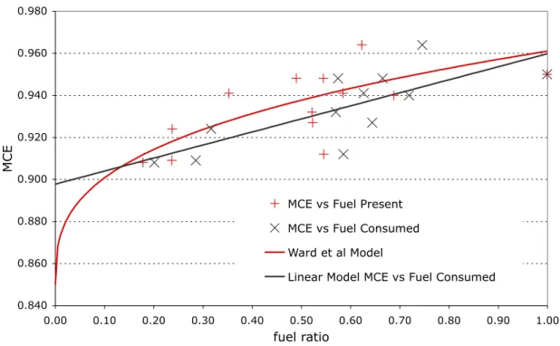
MCE is computed from a linear function of the ratio of com-busted woody to grass litter, derived from the data presented by Ward et al. (1996). We decided against using the original non-linear model by Ward et al. (1996), because it predicts MCE=0.85 when all litter is woody, which is much lower than the lowest ecosystem-specific value implied by the data of Andreae and Merlet (2001), which is 0.94 for extratrop-ical forests. Also, Ward et al. (1996) present no data for a woody litter fraction greater than 0.84 (fuel ratio<0.16, see Fig. A1). Their original model is based on fuel present at the sites, not the amount of fuel burnt in each fire. To obtain the amount of combusted fuel from their data, we assume that all grass present at the site burns completely, which is supported by a combustion factor of 1.0 for one site where almost all fuel is grass. It is also assumed that the combustion factors of all other fuel types than grass are the same. To obtain com-busted woody litter, the combustion factor for fuel other than grass is then calculated from the reported total combustion factor using the equationCng·(T′−G′)+G′=C·T′, where Cis total combustion factor,Cng non-grass combustion
fac-tor,T′total fuel present, andG′grass fuel present. We then useL=Cng·L′andG=G′to obtain combusted woody
lit-ter,L, and combusted grass,G, from woody litter (L′) and grass (G′) present at the site.
The linear model of the modified combustion efficiency derived from combusted fuel amounts is:
MCE=0.898+0.062·G/(G+L). (1) Emission factors as a function of MCE are taken from Ward et al. (1996) for CO, CH4, NMHCs and PM2.5. The equa-tion for NMHCs has been taken from Ward (2001), who cites Ward et al. (1996). We use the definition of the MCE to de-rive emissions of CO2 from emissions of CO as CO emis-sions times MCE/(1-MCE) times 44/28, where the latter is the ratio of molar masses of CO2and CO, respectively.
We use two further models for the emission of PM2.5based the work of Janh¨all et al. (2010). Emission Model 3 (EM3) uses a linear relationship between the emission factor for particle mass and MCE taken from Eq. (10) of Janh¨all et al. (2010), using the MCE from EM2 (see Fig. 1). The emis-sion factor for EM3, in g per kg dry mass, is:
EFPM2.5=86.1−85.3·MCE±3.1. (2)
Emission Model 4 (EM4) uses fixed emission factors for aerosol mass differentiated between forest, savanna and grass biomes (Janh¨all et al., 2010, Table 4). The values are 11±6, 6±3 and 5±2 g per kg dry mass, respectively. For EM4, the three biomes are determined from the simulated grass frac-tion of LAI as follows: “forest” for up to 20 %, “savanna” for greater than 20 % and up to 80 %, and “grass” for greater than 80 %.
2.4 Uncertainties
We assess the sensitivity of simulated emissions to changing parameters or input data sets by varying them within bounds consistent with available data or published estimates. The re-sulting uncertainties in emissions are intended as a first in-dication of their order of magnitude. We therefore neither attempt to rank those uncertainties, nor do we combine them to arrive at an overall uncertainty estimate.
Uncertainties in simulated emissions result from uncer-tainties in burned area, in the amount of combusted biomass on the burned surfaces, from differences between emission models, and from the uncertainties of the emission factor for a given model. All uncertainties are represented by chang-ing model parameters, except for those resultchang-ing from dif-ferences in estimated burned area. For this special case, we need to make assumptions about the spatial correlation of the error that leads to the difference between burned-area prod-ucts. At one extreme, we could assume that they are spa-tially uncorrelated at the grid cell level, in which case the global uncertainty would be the square root of the summed error variances over all grid cells. At the other extreme, we could compute the standard deviation after forming global sums of each simulation, assuming differences are entirely due to systematic errors. If, however, differences turned out to be purely random and uncorrelated between different grid cells, this latter approach would lead to a large underestimate of the uncertainty.
Here, we assume that the dominant contributing factor to uncertainties are systematic differences between methods of burned-area retrieval, but that the impact of these differences varies regionally. This is supported by the finding that mag-nitude and sign of differences between L3JRC, MODIS and GFED3 vary substantially between large regions, as does the difference to regional-scale burned-area data (Chang and Song, 2009). Therefore, we compute the uncertainty for each of the GFED basis regions (see Fig. A2) separately, and then use the square root of the squared sum as the global uncer-tainty estimate. For two regions, Boreal North America and Boreal Asia, we take the absolute difference between simu-lations with GFED3 and MCD45 as the uncertainty estimate. This is to avoid the extremely high burned areas by L3JRC for those regions. For all the others, we use the sample stan-dard deviation of the three simulations with different burned area products (usingn−1 in the denominator).
We further use the sample standard deviation, but based on global sums, for emissions of PM2.5, where there are four emission models available. For other species with only two emission models, we indicate the range between the high and the low estimate based on global sums. The same approach is used for indicating the uncertainty due to fuel combustion completeness, where the range between the high (cw=0.4) and the low esimate (cw=0.2) is taken. This assumes that the impact of uncertainties in ch on simulated emissions is small. For the uncertainty due to simulated fuel loads,
we give the range between the average of the two simula-tion with woody combussimula-tion factor 0.2 and 0.4 and standard turnover time for woody litter on the one hand, and the sim-ulation with adjusted woody litter turnover time and woody combustion factor of 0.3 on the other. While two to four sam-ples are certainly too few to derive a robust margin of error, this study nevertheless attempts to derive a first estimate of the contrasting contributors to uncertainties of wildfire chem-ical emissions.
To estimate the uncertainties resulting from the finite sam-ple size of emission factors measured in the field, we use the standard deviations of EM1 as reported by P. Merlet (per-sonal communication, 2008), with the following provisions: if error margins are not given (only one or no measurements), we use twice the higher relative standard deviation of the emission factors for the other ecosystems, as far as available, else four times the mean value. If uncertainties are given as a range (when only two measurements are available), we use twice the range. We further assume that the uncertainties of emission factors for different ecosystems are uncorrelated in order to derive spatial integrals of uncertainty.
3 Results
3.1 Simulated and observed fuel load
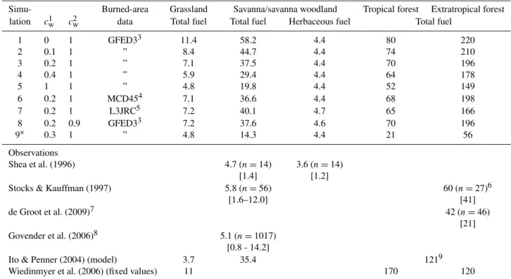
A set of nine global simulations was performed with the ecosystem model LPJ-GUESS, varying the combustion fac-tors for woody (cw), and for herbaceous fuel (ch), the burned-area input data, and the rate of decomposition of both lit-ter types as described in Sect. 2.1. The simulations are listed in Table 2, together with simulated and observed fuel loads for different biomes. Observations are pre-burn fuel loads from experimental fires or wildfires, simulations the average weighted by burned area over all simulation years, all in tons dry mass per hectare. In those cases where only ranges of ob-served values are given, we assume the mean to equal the av-erage of the minimum and maximum reported values. For the simulations, the definition of the biomes follows that used by the emission models: grassland with<20 % LAI fraction of trees, savanna/savanna woodland between 20 and 80 %, and forests above that number. Tropical forests are those where the dominant PFT is a tropical tree. The table also shows the assumptions used by Wiedinmyer et al. (2006) and the results of the data-based modelling study by Ito and Penner (2004). We find that Simulations 3 and 4, representing the assumed range of the wood combustion factor, approximately repro-duce the data-based simulations by Ito and Penner (2004) for savannas and forests, but overestimate woody litter in grass-lands. Simulated grassland fuel load is also rather sensitive to
Table 2. Simulations with LPJ-GUESS, simulated and observed fuel loads in t dry matter/ha.
Simu- Burned-area Grassland Savanna/savanna woodland Tropical forest Extratropical forest
lation c1w cw2 data Total fuel Total fuel Herbaceous fuel Total fuel
1 0 1 GFED33 11.4 58.2 4.4 80 220
2 0.1 1 ” 8.4 44.7 4.4 74 210
3 0.2 1 ” 7.1 37.5 4.4 70 196
4 0.4 1 ” 5.9 29.4 4.4 64 178
5 1 1 ” 4.8 19.8 4.4 52 149
6 0.2 1 MCD454 7.1 36.6 4.4 68 198
7 0.2 1 L3JRC5 7.2 40.1 4.7 65 166
8 0.2 0.9 GFED33 7.2 37.6 4.6 70 196
9∗ 0.3 1 ” 4.8 14.3 4.4 21 56
Observations
Shea et al. (1996) 4.7 (n=14) 3.6 (n=14)
[1.4] [1.2]
Stocks & Kauffman (1997) 5.8 (n=56) 60 (n=27)6
[1.6–12.0] [41]
de Groot et al. (2009)7 42 (n=46)
[21]
Govender et al. (2006)8 5.1 (n=1017)
[0.8 - 14.2]
Ito & Penner (2004) (model) 3.7 35.4 1219
Wiedinmyer et al. (2006) (fixed values) 11 170 120
Values in [...] are range or standard deviation.∗Woody litter turnover time changed from 20 to 4 yr.1Combustion factor for woody litter.2Combustion factor for herbacous
litter.39/1996–12/2009.4MODIS 4/2000–12/2009.54/2000–3/2007.6Data for Canada. Inferred from fuel load divided by combustion completeness (CC); CC range translated to standard deviation assuming range corresponds to normal distribution between 1/nand (n−1)/nfractiles.7Table 3, excl. open woodland category.8Table 4, excl. Shea et al. (1996).9Both forest categories.
total fuel load compared to the field data, even if 100 % combustion is assumed for both litter categories (Simula-tion 5). By contrast, simulated fuel loads with the excep(Simula-tion of tropical forests are lower than those used by Wiedinmyer et al. (2006).
For Simulation 9, where litter decomposition rates were delibrately adjusted to better match field-observed total fuel in extratropical forests, total fuel load in savannas and sa-vanna woodlands is still higher than observed. For all sim-ulations, simulated herbaceous fuel in savannas is lower but still in reasonable agreement with observations. The com-bustion factor for herbaceous fuel has only a small impact on simulated fuel load when varied within plausible bounds (Simulation 3 vs. 8).
The use of L3JRC burned area leads to considerably lower simulated fuel loads in extratropical forests due to higher burned area (Simulations 3 and 7), more than the effect of doubling the wood combustion factor (Simulations 3 and 4). In savannas, use of L3JRC increases simulated fuel loads due to the lower burned area in the relevant areas (Giglio et al., 2010). Results with the other two burned area products are very similar between each other.
3.2 Sensitivity to combustion factor and fuel load
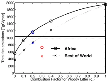
Simulated carbon emissions from wildfires – independent of chemical species, computed before the application of one of the emission models – are highly sensitive to the choice of the combustion factor for woody fuel (Fig. 2). Within the plausi-ble range ofcwbetween 0.2 and 0.4, fire emissions increase by approximately 25 % for Africa and 40 % for the remaining part of the globe. We find a non-linear relationship with di-minishing returns, which we attribute to the effect of repeated fires. If we assume that all woody fuel not consumed in a sin-gle fire year eventually decomposes, we would expect a lin-ear increase between the points withcw=0 and 1. The simu-lated amount, however, is considerably higher for intermedi-ate values. The impact of the non-linear response is also more pronounced for Africa (difference of 364 TgC yr−1or 25 % of emissions against linear response atcw=0.4, compared
to 224 TgC yr−1or 18 % for rest-of-world, Fig. 2), which we attribute to the higher fire frequency in Africa.
0 0.1 0.2 0.3 0.4 0.5 0.6 0.7 0.8 0.9 1 0
200 400 600 800 1000 1200 1400 1600 1800 2000
Combustion Factor for Woody Litter (cw)
Total fire emissions [TgC/year]
Africa
Rest of World
Fig. 2.Sensitivity of average global fire emissions 1997–2009. The horizontal lines show GFED3 emissions during the same period. Blue symbols: combustion efficiency for herbaceous fuel reduced from 1 to 0.9. Red symbols: litter turnover adjusted to match ob-served fuel loads.
but the one with faster woody litter turnovercw=0.3. The contribution of herbaceous fuel can be inferred from emis-sions at the pointcw=0: those emissions contribute about
half (atcw=0.2) to one third (cw=0.4) to the global total.
We also find that the value ofcw=0.2 (Simulation 3 of Table 2) with GFED3 burned area gives results that are clos-est to the emission clos-estimates of GFED3 (Fig. 2). This value of 0.2 is retained throughout the remainder of this text and for further sensitivity analyses, where dependence of emissions of chemical species on burned area observations or emission model are considered.
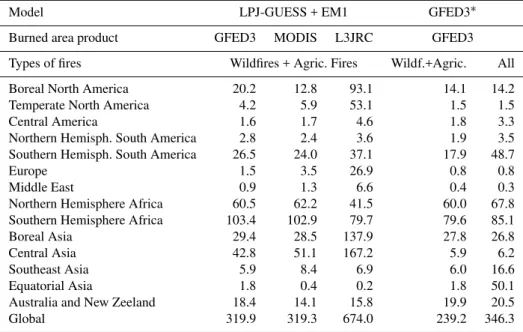
Another way of assessing the impact of different combus-tion factors and fuel loads is to compare the simulated emis-sions with GFED3 burned area and EM1 with those com-puted by van der Werf et al. (2010), who used the same burned-area data and emission model. While LPJ-GUESS simulates the vegetation present at each site as natural vege-tation, the CASA model as used by van der Werf et al. (2010) uses observed vegetation distribution as an external input to the model. CASA also includes peat fires, deforestation and agricultural waste burning explicitly, while LPJ-GUESS sim-ulates all observed fires as wildfires with no live biomass burned. In the case of deforestation fires, this leads to an un-derestimate of emissions because felling and burning of trees is not simulated. Table 3 shows the LPJ-GUESS and GFED3 CO emissions for wildfires and agricultural burning, as well as total emissions for GFED3. For a definition of the regions see (Giglio et al., 2010) and Fig. A2.
Global emissions are 33 % higher for LPJ-GUESS com-pared to GFED3, about equal for Northern Hemisphere Africa, and 30 % higher for Southern Hemisphere Africa. Boreal North America is also higher by 43 %, while Boreal Asia is in close agreement. Southeast and Equatorial Asia are
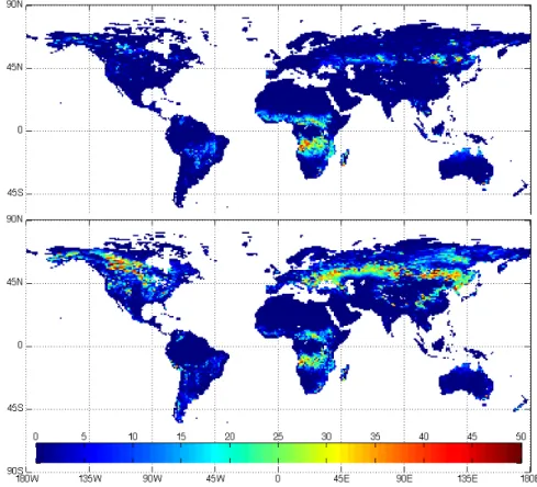
again somewhat higher for LPJ-GUESS when only consider-ing wildfires and agricultural burnconsider-ing, but here the GFED3 total emissions are much higher due to the contribution from peat fires. The region that stands out in this comparison is Central Asia, where LPJ-GUESS emissions are an order of magnitude higher than GFED3. As Fig. 3 reveals, the region (cf. Fig. A2) has high simulated CO emissions especially in regions known to be dominated by agricultural fields (Ra-mankutty and Foley, 1999). One explanation for the discrep-ancy in emissions is that LPJ-GUESS simulates only poten-tial natural vegetation, leading to overestimated fuel loads. This also explains why Europe and Temperate North Amer-ica have much higher simulated emissions for LPJ-GUESS. There is, however, reasonable agreement for the major emis-sion regions, such as Africa, Australia, and South America.
3.3 Sensitivity to burned area
With a much different burned area detection algorithm than GFED3 or MODIS MCD45 (Roy and Boschetti, 2009), the L3JRC product (Tansey et al., 2008) leads to much higher emissions in the mid to high latitudes (Boreal and Temper-ate North America, Europe, Boreal and Central Asia; Ta-ble 3). The differences are by order of magnitude of emis-sions, as opposed to the much smaller differences between the two MODIS or predominantly MODIS-based products. For Africa, however, L3JRC emissions are somewhat lower than MODIS or GFED3 emissions, which corresponds to lower burned area in the region (Roy and Boschetti, 2009). MODIS and GFED3, on the other hand, are again very simi-lar for this region.
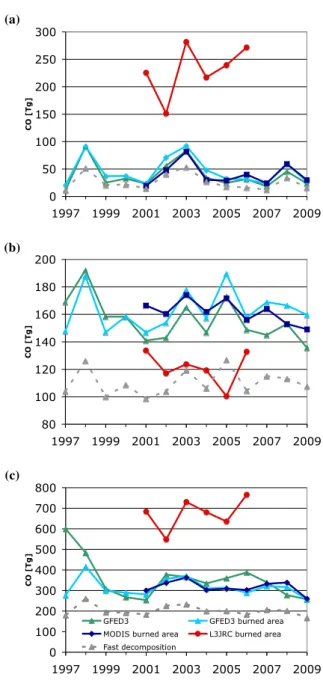
A comparison shown in Fig. 4 reveals not only large dif-ferences in magnitude but also in interannual variability be-tween simulations with different burned area data. For ex-ample, for Africa (Fig. 4a), interannual variability is much larger for MODIS (standard deviation 2001–2009: 13.1 Tg) than for GFED3 burned area (8.3 Tg). For L3JRC, even tem-poral maxima and minima change sign compared to the other products: note for example that 2005 for Africa is a minimum for L3JRC, and a maximum for the other products, or 2002 in the boreal zone, which is a pronounced temporal minimum in L3JRC, but not for any of the other data sets (Fig. 4a, b). On a global scale (Fig. 4c), GFED3 and MODIS lead to very similar results, however, with L3JRC standing out as much higher. The difference between GFED3 emissions and emis-sions from LPJ-GUESS with GFED3 burned area for 1997 can be attributed again to peat fires, which were especially wide-spread during the 1997/1998 El Ni˜no (Page et al., 2002; Langenfelds et al., 2002).
Fig. 3.CO emissions in gC m−2yr−1forcw=0.2 and Emission Model 1, average 2001–2006. Upper panel: GFED3 burned area. Lower panel: L3JRC burned area.
regional breakdown of the emissions (Table 3) also shows great similarity between GFED and MODIS, with the ex-ception of some areas with minor contributions: Equatorial Asia, notably Boreal North America, where MODIS is close to half of GFED3, and Europe and Southeast Asia where this difference is reversed. The different burned area for Equa-torial Asia was already noted by Giglio et al. (2010), where GFED3 reports generally much higher values. This was at-tributed to a mapping algorithm more resistant to cloud and aerosol contamination, leaving fewer undetected burned pix-els.
3.4 Emission models
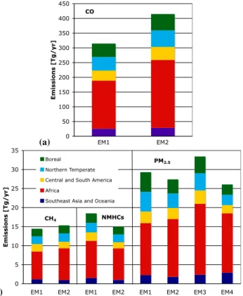
Simulated emissions are found to be rather sensitive to the choice of emission model, as is shown in Fig. 5. Annual car-bon emissions for EM1 are 6655 Tg CO2(92.9 % of carbon emissions), 315 Tg CO (6.8 %), 14 Tg methane (0.5 %) and 18 Tg non-methane hydrocarbons (0.6 %), whereas for EM2 the figures are 8886 Tg CO2 (90.4 %), 415 Tg CO (8.6 %), 15 Tg methane (0.6 %), and 15 Tg NMHCs (0.4 %). The cal-culation assumes an average molar mass per carbon atom of 20 g for NMHCs derived from the data by P. Merlet (personal communication, 2008) for tropical grasslands and savannas. EM2 thus predicts a considerably lower combustion effi-ciency for wildfires with much higher CO emissions, while
EM1 yields a smaller combustion efficiency, but with fires producing considerably more NMHCs relative to methane.
In general, the choice of emission model impacts more the magnitude and less the geographical breakdown of emissions (Fig. 5). At least for CO and methane, the share of emissions going to Africa is somewhat higher for EM2 (CO: 56 %, methane: 55 %) than for EM1 (CO: 52 %, methane: 51 %). For aerosols (PM2.5), there are also some notable redistri-butions in emissions: For EM4, most emissions come from Africa (60 %) and Southeast Asia and Oceania (11 %), with the boreal and temperate zones only contributing 10 % each. EM1, at the other end of the spectrum, allocates only 47 % to Africa, but 18 % each to the boreal and temperate zones, and only 8 % to Southeast Asia and Oceania. We further find that choice of emission model generally has only a small effect on interannual variations of emissions (results not shown).
3.5 Contributions to emission uncertainties
(a)
0 50 100 150 200 250 300
1997 1999 2001 2003 2005 2007 2009
CO
[
Tg
]
(b)
80 100 120 140 160 180 200
1997 1999 2001 2003 2005 2007 2009
CO
[
Tg
]
(c)
0 100 200 300 400 500 600 700 800
1997 1999 2001 2003 2005 2007 2009
CO [Tg]
GFED3 GFED3 burned area
MODIS burned area L3JRC burned area
Fast decomposition
Fig. 4. Annual CO emissions in Tg for cw=0.2 and Emission Model 1, for different burned area data sets and for fast litter decom-position, as well as GFED3 emissions.(a)Boreal Asia and North America.(b)Africa.(c)Globe.
include an estimate of overall uncertainty, nor do we base our best guess on the average across emission models and burned area products.
Considering only orders of magnitude, we find that the dif-ferent factors contribute about equal levels of uncertainty to the simulated emissions. Only for CO2, the emission model has a minor effect on uncertainties. Notable is a rather high contribution from simulated fuel loads.
There are cases, however, where emission factor uncer-tainty has a similar or larger impact on emissions than any of the other factors. The simulated emissions of propane, SO2,
xylenes, ethanol and acetaldehyde depend more strongly on uncertainties in emission model than on fuel load and com-bustion. Propane has a much higher emission factor for trop-ical forest (1.04 kg g−1dry matter, P. Merlet, personal com-munication, 2008) than for savanna and grassland (0.086) or extratropical forest (0.27), but this high factor for tropical forests is based on only two measurements. Xylenes have the highest estimated emission factor for extratropical forest (0.2) based on only one measurement (vs. 0.043 and 0.087 for the other biomes), and ethanol has only one measure-ment for extratropical forest and none for the other ecosys-tems. For acetaldehyde, the situation is similar to propane, with only two measurements from tropical forests, but a more than four times higher emission factor than for savannas and grasslands. Other cases with relatively large uncertainties due to emission factors are NOx, NH3, ethene, propene, benzene, toluene, methanol, formaldehyde, and acteone.
We find a remarkably large difference between the two emission models for CO, resulting in a range of 100 Tg yr−1, twice as much as the effect of the uncertainty of the emis-sion factor of EM1. We combine both emisemis-sion factor and emission model uncertainty and assume they are uncorre-lated to derive the overall influence on uncertainties through the choice of emission model. We thus arrive at the follow-ing indicative esimates for the five main groups of emitted species (CO2, CO, CH4, NHMCs and particulate matter): about 50 % estimated uncertainty from fuel load, 30 to 40 % from fuel combustion, 25 % from burned area, and 20 to 30 % from emissions modelling. Exceptions are CO2, with 5 %, and CO with 36 % uncertainty from emission modelling.
4 Discussion
Even though some of the results have been presented in terms of uncertainties, it must be stressed that the reported ranges are only first estimates. These estimates have been derived from what is essentially a sensitivity analysis of chemical emissions from wildfires to plausible scenarios of parameter, model or input data choice. The first issue to discuss is there-fore how the models used here compare with other global modelling efforts of wildfire emissions.
Table 3.Average annual CO emissions in Tg 2001–2006 with LPJ-GUESS and Emission Model 1 using different remotely sensed burned area products: GFED3 (Giglio et al., 2010), L3JRC (Tansey et al., 2008), and MODIS MCD45 (Roy et al., 2005). Last 2 columns show emissions by GFED3. Wildfires (Wildf.) exclude deforestation, peat fires and agricultural waste burning (Agric.).
Model LPJ-GUESS + EM1 GFED3∗
Burned area product GFED3 MODIS L3JRC GFED3
Types of fires Wildfires + Agric. Fires Wildf.+Agric. All
Boreal North America 20.2 12.8 93.1 14.1 14.2
Temperate North America 4.2 5.9 53.1 1.5 1.5
Central America 1.6 1.7 4.6 1.8 3.3
Northern Hemisph. South America 2.8 2.4 3.6 1.9 3.5
Southern Hemisph. South America 26.5 24.0 37.1 17.9 48.7
Europe 1.5 3.5 26.9 0.8 0.8
Middle East 0.9 1.3 6.6 0.4 0.3
Northern Hemisphere Africa 60.5 62.2 41.5 60.0 67.8
Southern Hemisphere Africa 103.4 102.9 79.7 79.6 85.1
Boreal Asia 29.4 28.5 137.9 27.8 26.8
Central Asia 42.8 51.1 167.2 5.9 6.2
Southeast Asia 5.9 8.4 6.9 6.0 16.6
Equatorial Asia 1.8 0.4 0.2 1.8 50.1
Australia and New Zeeland 18.4 14.1 15.8 19.9 20.5
Global 319.9 319.3 674.0 239.2 346.3
∗van der Werf et al. (2010).
GFED3. Based on those comparisons, we would expect the emissions of Simulation 9 to be too low.
There might be a number of factors contributing to this ap-parent contradiction. Firstly, fuel loads in savannas strongly depend on mean annual rainfall (Govender et al., 2006), and the precipitation data used by LPJ-GUESS has to rely on a rather sparse network of stations in most of those areas (Mitchell and Jones, 2005). Also, the LAI fraction of trees and shrubs assumed in this study for the savanna/savanna woodland category (20 to 80 %) is somewhat higher then that assumed for example by the International Geosphere Bio-sphere Program (10 to 60 %, Friedl et al., 2002). Simulated total fuel in LPJ-GUESS is similar to other modelling stud-ies, but should be thought of as representing not only surface fuels, but also fuels in killed shrubs or short trees, for exam-ple, that contribute to emissions but are not captured by the field data cited. It could also represent collected fuel wood (van der Werf et al., 2010), which was estimated to amount to 10 % of savanna emissions in Africa (Williams et al., 2007). Fuel wood likewise contributes to emissions but does not ap-pear in fuel load data for African savannas. Possibly, LPJ-GUESS effectively accounts for these effects by assuming a higher woody fuel load than is in fact found on the ground.
Another explanation, which has been discussed before, states that part of what is simulated as fuel in LPJ-GUESS is wood contained in dead standing trees that do not burn or contribute to emissions. If we assume half of the modelled woody fuel is indead standing trees and halve the combus-tion factor for woody fuel from the plausible range of 0.2 to
0.4 to values between 0.1 and 0.2, we obtain the following results (Simulations 2 and 3, see Table 2): simulated woody fuel in savannas is between 33 and 40 t/ha, and surface litter between 16 and 20 t/ha. Simulation 3, resulting in 16 t/ha, also has similar emissions to GFED3. While this is still too high compared to observations, a combination of both pro-posed factors, a systematic difference in the tree fraction tween simulations and observations, and possible biases be-tween actual and observed rainfall might be able to explain the difference.
Table 4.Global wildfire emissions in Tg yr−1with Emission Model 1,cw=0.2 and GFED3 burned area (best guess), and uncertainties from various factors. “Higher alkenes” and “higher alkanes” with a least 4 C atoms. OC: organic carbon. BC: black carbon. NMHCs: non-methane hydrocarbons. TPM: total particulate matter. PM2.5particulate matter up to 2.5 micron.
Uncertainty resulting from:
Species Best guess1 emission factor1 emission model1 fuel combustion1 fuel load1 burned area2
CO2 6656 271 230 2123 3273 1681
CO 315 50 100 112 169 79
CH4 14.4 2.8 0.9 5.6 8.2 3.2
NMHCs 18.5 4.9 3.5 6.7 10.0 4.3
TPM 44.2 10.2 – 15.8 23.7 12.1
PM2.5 29.3 6.8 3.7 11.0 16.3 8.0
NOx 9.75 3.45 – 3.30 5.03 2.65
N2O 0.89 0.30 – 0.29 0.44 0.23
NH3 3.85 1.77 – 1.37 2.07 1.08
SO2 2.26 3.09 – 0.85 1.26 0.61
OC 18.4 4.1 – 6.8 10.2 5.5
BC 2.04 0.52 – 0.68 1.04 0.52
ethene 4.20 1.43 – 1.48 2.23 0.99
ethane 2.24 0.65 – 0.89 1.30 0.47
propene 2.20 0.78 – 0.85 1.25 0.43
propane 1.25 2.82 – 0.56 0.79 0.16
higher alkenes 2.01 0.45 – 0.71 1.07 0.50
higher alkanes 0.78 0.19 – 0.29 0.44 0.22
benzene 1.40 0.57 – 0.49 0.75 0.38
toluene 0.95 0.46 – 0.34 0.51 0.26
xylenes 0.33 0.31 – 0.13 0.19 0.10
methanol 7.50 3.66 – 2.68 4.00 1.67
ethanol 0.05 0.06 – 0.02 0.03 0.01
formaldehyde 5.18 2.12 – 2.06 3.02 1.25
acetaldehyde 3.80 2.55 – 1.54 2.23 0.69
acetone 2.22 0.79 – 0.76 1.15 0.56
11997–2009.22001–2006. Range based on two samples shown initalics.
out that other factors than fuel composition or biome are bet-ter predictors.
The remaining question is whether the rather wide range of burned-area estimates used in this study (L3JRC was ex-cluded for the boreal zone) can be considered a plausible uncertainty estimate. Had we used only L3JRC and MCD45, the burned-area based uncertainty of CO2 emission would have dropped from 1680 to 240 TgC yr−1. However, both these data sets are mainly based on data from the same satellite sensor, so that the regional differences between the two cannot be expected to be a good estimator of uncer-tainties. For example, Chang and Song (2009) showed that MCD45 underestimates monthly burned area by 44 % for Canada, 53 % for the United States (US), and 27 % for China against regional estimates. On the other hand, L3JRC over-estimates by factors of 1.5 and 4 for US and China, respec-tively (for Canada and Alaska, L3JRC does not enter the un-certainty calculation). For Africa, however, L3JRC underes-timates burned area compared to analyses of high-resolution
images (Roy and Boschetti, 2009). We therefore assume that the uncertainty estimate for the impact of burned area is rea-sonable, even if somewhat high.
A new finding is that there is not only a large bias be-tween L3JRC and the other two satellite products, but that interannual variability simulated using L3JRC differs signif-icantly from using the predominantly MODIS-based prod-ucts. Therefore, further validation of satellite burned area also needs to consider how reliably interannual variations are reproduced.
(a) 0
50 100 150 200 250 300 350 400 450
EM1 EM2
Emissio
ns [T
g/yr]
CO
(b)
0 5 10 15 20 25 30 35
EM1 EM2 EM1 EM2 EM1 EM2 EM3 EM4
Emissio
ns [Tg/yr]
Boreal
Northern Temperate
Central and South America
Africa
Southeast Asia and Oceania
CH4 NMHCs
PM2.5
Fig. 5.Average emissions 1997–2009 region of (a) CO; and of (b)methane, non-methane hydrocarbons (NMHCs) and aerosol par-ticulate matter up to 2.5 microns. Emissions are forcw=0.2 and different emission model (EM). Boreal: Boreal North America and Boreal Asia. Northern Temperate: Temperate North America, Eu-rope, Middle East and Central Asia. Southeast Asia and Oceania: Southeast Asia, Equatorial Asia and Australia and New Zealand.
has areas with values between 5 and 10 % yr−1, with the rest of the region closer to 1 % yr−1. By comparison, African sa-vannas burn between 10 and 30 % of their area each year. While the model by Thonicke et al. (2010) is more pro-cess based, Kloster et al. (2010) show results of simulated burned area using the much simpler approaches of Thon-icke et al. (2001) and Arora and Boer (2005) and find rea-sonable broad agreement with L3JRC and GFED2 (Giglio et al., 2006). However, Giglio et al. (2010) found that GFED3 agrees substantially better with independent data than either GFED2 or L3JRC. This has consequences for model eval-uation: for example, the model by Arora and Boer (2005) simulates twice to 6 times the GFED2 burned area for Eu-rope, but GFED3 has 75 % less burned area in the same re-gion than GFED2 (Giglio et al., 2010). Because no model-predicted burned area can be expected to have lower uncer-tainty than the best observations – as they rely on observa-tional evidence for their design – we believe that further vali-dation and improvement of remotely sensed products is nec-essary for improved prediction of burned area and fire emis-sions. Apart from that, we need further efforts for designing, parameterising and refining predictive fire models that can
be tested against burned-area observations at various spatial scales (Lehsten et al. 2010).
Overall, we find that in order to arrive at a predictive ca-pability for the impacts of climate change on wildfire emis-sions, the main priority is to obtain more data on combus-tion factors and in particular factors that characterize the as-sociated weather and fuel moisture conditions, as the cur-rently available data seriously limit modelling capability (Ito and Penner, 2004; Wiedinmyer et al., 2010). This includes improved precipitation data as the main driver for fuel load (Govender et al. 2006). The next highest priority would be a systematic comparison of global and regional data on burned area, and a systematic improvement of burned-area models to better match well-validated observations. Finally, the range of emissions reported here could not only be tested against atmospheric inversions of relatively long-lived chemical trac-ers such as CO (Kopacz et al., 2010), but ultimately parame-ters of the emission model could be constrained directly via inverse modellling, similar to the technique used in Carbon Cycle Data Assimilation (Rayner et al., 2005).
5 Conclusions
We have presented a framework for exploring the sensitivity of global chemical emissions from wildfires to various un-certain model inputs and parameterisations. Simulated fuel loads were comparable to other modelling studies, but higher than observed for African savannas. We have dicusssed sev-eral factors that could explain the difference. We concluded that modelled fuel loads still contribute to a large uncertainty in the estimated wildfire emissions.
The study futher highlights the need for models of com-bustion completeness as a function of climatic conditions, possibly in conjunction with reliable models of fire intensity, and the need for better models of emission factors for several species. For the main emitting species, however, the main issue is accurate modelling of burned area and combusted biomass, crucial for assessing fire emissions in past or future environments.
Our results can be used by the atmospheric modelling community to consider a range of emission scenarios rather than a fixed one, reflecting the uncertainty range due to current modelling capabilities. Modelling different emission scenarios together with chemical transport can be used to further constrain emissions, given suitable observations and long-lived tracers.
We conclude that model-based prediction of chemical emissions from wildfire, either for present or future condi-tions, still carries a high degree of uncertainty.
0.840 0.860 0.880 0.900 0.920 0.940 0.960 0.980
0.00 0.10 0.20 0.30 0.40 0.50 0.60 0.70 0.80 0.90 1.00
fuel ratio
MCE
MCE vs Fuel Present
MCE vs Fuel Consumed
Ward et al Model
Linear Model MCE vs Fuel Consumed
Fig. A1.Models of Modified Combustion Efficiency (MCE) against fuel ratio according to Ward et al. (1996) and derived as in the main text, as well as measured MCE by Ward et al. (1996) versus fuel ratio for either fuel present before the fire, or fuel consumed during the fire. The Ward et al model is a function of the fuel ratio of the fuel present, the linear MCE model derived here a function of the fuel ratio of the fuel consumed. The fuel ratio is defined as the amount of grass fuel (live grass and grass litter) divided by total fuel amount (including non-grass debris).
Acknowledgements. This work was supported by EU contracts 265148 (Pan-European Gas-Aerosol-climate interation Study, PEGASOS), and 243888 (Forest fires under climate, social and economic changes in Europe, the Mediterranean and other fire-affected areas of the world, FUME). The authors would like to thank Claire Granier for suggestions on which chemical species to include, and two anonymous reviewers for their critical comments, which we believe have helped to greatly improve the manuscript.
Edited by: K. Carslaw
References
Andreae, M. O. and Merlet, P.: Emission of trace gases and aerosols from biomass burning, Global Biogeochem. Cy., 15, 955–966, 2001.
Arneth, A., Harrison, S. P., Zaehle, S., Tsigaridis, K., Menon, S., Bartlein, P. J., Feichter, J., Korhola, A., Kulmala, M., O’Donnell, D., Schurgers, G., Sorvari, S., and Vesala, T.: Terrestrial biogeo-chemical feedbacks in the climate system, Nat. Geosci., 3, 525– 532, doi:10.1038/Ngeo905, 2010.
Arora, V. K. and Boer, G. J.: Fire as an interactive component of dynamic vegetation models, J. Geophys. Res., 110, G02008, doi:10.1029/2005jg000042, 2005.
Boschetti, L. and Roy, D. P.: Strategies for the fusion of satel-lite fire radiative power with burned area data for fire ra-diative energy derivation, J. Geophys. Res., 114, D20302, doi:10.1029/2008jd011645, 2009.
Bowman, D. M. J. S., Balch, J. K., Artaxo, P., Bond, W. J., Carlson, J. M., Cochrane, M. A., D’Antonio, C. M., DeFries, R. S., Doyle, J. C., Harrison, S. P., Johnston, F. H., Keeley, J. E., Krawchuk, M. A., Kull, C. A., Marston, J. B., Moritz, M. A., Prentice, I. C., Roos, C. I., Scott, A. C., Swetnam, T. W., van der Werf, G. R., and Pyne, S. J.: Fire in the Earth System, Science, 324, 481–484, doi:10.1126/Science.1163886, 2009.
Chang, D. and Song, Y.: Comparison of L3JRC and MODIS global burned area products from 2000 to 2007, J. Geophys. Res-Atmos., 114, D16106, doi:10.1029/2008jd011361, 2009. de Groot, W. J., Pritchard, J. M., and Lynham, T. J.: Forest floor
fuel consumption and carbon emissions in Canadian boreal for-est fires, Can. J. Forfor-est. Res., 39, 367–382, doi:10.1139/X08-19, 2009.
Duncan, B. N., Martin, R. V., Staudt, A. C., Yevich, R., and Logan, J. A.: Interannual and seasonal variability of biomass burning emissions constrained by satellite observations, J. Geophys. Res., 108, 4100, doi:10.1029/2002jd002378, 2003.
Ellicott, E., Vermote, E., Giglio, L., and Roberts, G.: Estimating biomass consumed from fire using MODIS FRE, Geophys. Res. Let., 36, L13401, doi:10.1029/2009gl038581, 2009.
Etheridge, D. M., Steele, L. P., Langenfelds, R., and Francey, R. J.: Natural and anthropogenic changes in atmospheric CO2over the last 1000 years from air in Antarctic ice and firn, J. Geophys. Res., 101, 4115–4128, 1996.
Friedl, M. A., McIver, D. K., Hodges, J. C. F., Zhang, X. Y., Mu-choney, D., Strahler, A. H., Woodcock, C. E., Gopal, S., Schnei-der, A., Cooper, A., Baccini, A., Gao, F., and Schaaf, C.: Global land cover mapping from MODIS: algorithms and early results, Remote Sens. Environ., 83, 287–302, 2002.
Gr´egoire, J. M., Tansey, K., and Silva, J. M. N.: The GBA2000 initiative: developing a global burnt area database from SPOT-VEGETATION imagery, Int. J. Remote Sens., 24, 1369–1376, doi:10.1080/0143116021000044850, 2003.
Giglio, L., van der Werf, G. R., Randerson, J. T., Collatz, G. J., and Kasibhatla, P.: Global estimation of burned area using MODIS active fire observations, Atmos. Chem. Phys., 6, 957– 974, doi:10.5194/acp-6-957-2006, 2006.
Giglio, L., Randerson, J. T., van der Werf, G. R., Kasibhatla, P. S., Collatz, G. J., Morton, D. C., and DeFries, R. S.: Assess-ing variability and long-term trends in burned area by mergAssess-ing multiple satellite fire products, Biogeosciences, 7, 1171–1186, doi:10.5194/bg-7-1171-2010, 2010.
Gobron, N., Pinty , B., Melin, F., Taberner , M., Verstraete, M. M., Robustelli, M., and Widlowski, J.-L.: Evaluation of the MERIS/ENVISAT FAPAR product, Adv. Space Res., 39, 105– 115, 2007.
Govaerts, Y., Pereira, J. M., Pinty, B., and Mota, B.: Impact of fires on surface albedo dynamics over the African continent, J. Geo-phys. Res., 107, 4629, doi:4610.1029/2002JD002388, 2002. Govender, N., Trollope, W. S. W., and Van Wilgen, B. W.: The effect
of fire season, fire frequency, rainfall and management on fire intensity in savanna vegetation in South Africa, J. Appl. Ecol., 43, 748–758, doi:10.1111/J.1365-2664.2006.01184.X, 2006. Hoelzemann, J. J., Schultz, M. G., Brasseur, G. P., Granier, C., and
Simon, M.: Global Wildland Fire Emission Model (GWEM): Evaluating the use of global area burnt satellite data, J. Geophys. Res., 109, D14S04, doi:10.1029/2003jd003666, 2004.
Ito, A. and Penner, J. E.: Global estimates of biomass burning emis-sions based on satellite imagery for the year 2000, J. Geophys. Res., 109, D14S05, doi:10.1029/2003jd004423, 2004.
Janh¨all, S., Andreae, M. O., and P¨oschl, U.: Biomass burning aerosol emissions from vegetation fires: particle number and mass emission factors and size distributions, Atmos. Chem. Phys., 10, 1427–1439, doi:10.5194/acp-10-1427-2010, 2010. Jones, P. D. and Harris, I.: CRU Time Series (TS) high resolution
gridded datasets, NCAS British Atmospheric Data Centre, 2011. Keeling, C. D., Whorf, T. P., Wahlen, M., and Vanderplicht, J.: Inter-annual extremes in the rate of rise of carbon dioxide since 1980, Nature, 375, 666–670, 1995.
Kloster, S., Mahowald, N. M., Randerson, J. T., Thornton, P. E., Hoffman, F. M., Levis, S., Lawrence, P. J., Feddema, J. J., Ole-son, K. W., and Lawrence, D. M.: Fire dynamics during the 20th century simulated by the Community Land Model, Biogeo-sciences, 7, 1877–1902, doi:10.5194/Bg-7-1877-2010, 2010. Kopacz, M., Jacob, D. J., Fisher, J. A., Logan, J. A., Zhang, L.,
Megretskaia, I. A., Yantosca, R. M., Singh, K., Henze, D. K., Burrows, J. P., Buchwitz, M., Khlystova, I., McMillan, W. W., Gille, J. C., Edwards, D. P., Eldering, A., Thouret, V., and Nedelec, P.: Global estimates of CO sources with high resolu-tion by adjoint inversion of multiple satellite datasets (MOPITT, AIRS, SCIAMACHY, TES), Atmos. Chem. Phys., 10, 855–876, doi:10.5194/acp-10-855-2010, 2010.
Langmann, B., Duncan, B., Textor, C., Trentmann, J., and van der Werf, G. R.: Vegetation fire emissions and their impact on air pollution and climate, Atmos. Environ., 43, 107–116, 2009. Lehsten, V., Tansey, K., Balzter, H., Thonicke, K., Spessa, A.,
Weber, U., Smith, B., and Arneth, A.: Estimating carbon emissions from African wildfires, Biogeosciences, 6, 349–360, doi:10.5194/bg-6-349-2009, 2009.
Lehsten, V., Harmand, P., Palumbo, I., and Arneth, A.: Mod-elling burned area in Africa, Biogeosciences, 7, 3199–3214, doi:10.5194/Bg-7-3199-20, 2010.
Matson, M. and Dozier, J.: Identification of Subresolution High-Temperature Sources Using a Thermal Ir Sensor, Photogramm. Eng. Rem. S, 47, 1311–1318, 1981.
Mieville, A., Granier, C., Liousse, C., Guillaume, B., Mouillot, F., Lamarque, J. F., Gr´egoire, J. M., and Petron, G.: Emissions of gases and particles from biomass burning during the 20th cen-tury using satellite data and an historical reconstruction, Atmos. Environ., 44, 1469–1477, 2010.
Mitchell, T. D. and Jones, P. D.: An improved method for construct-ing a database of monthly climate observations and associated high-resolution grids, Int. J. Climatol., 25, 693–712, 2005. Mouillot, F. and Field, C. B.: Fire history and the global
car-bon budget: a 1 degrees×1 degrees fire history reconstruc-tion for the 20th century, Glob. Change Biol., 11, 398–420, doi:10.1111/J.1365- 2486.2005.00920.X, 2005.
Mutlu, M., Popescu, S. C., Stripling, C., and Spencer, T.: Mapping surface fuel models using lidar and multispectral data fusion for fire behavior, Remote Sens. Environ., 112, 274–285, 2008. Page, S. E., Siegert, F., Rieley, J. O., Boehm, H.-D. V., Jayak, A.,
and Limink, S.: The amount of carbon released from peat and forest fires in Indonesia during 1997, Nature, 420, 61–65, 2002. Prentice, I. C., Kelley, D. I., Foster, P. N., Friedlingstein, P.,
Har-rison, S. P., and Bartlein, P. J.: Modeling fire and the terres-trial carbon balance, Global Biogeochem. Cy., 25, GB3005, doi:10.1029/2010gb003906, 2011.
Ragland, K. W. and Aerts, D. J.: Properties of wood for combustion analysis, Bioresource Technol., 37, 161–168, 1991.
Ramankutty, N. and Foley, J. A.: Estimating historical changes in global land cover: Croplands from 1700 to 1992, Global Bio-geochem. Cy., 13, 997–1027, 1999.
Rayner, P. J., Scholze, M., Knorr, W., Kaminski, T., Giering, R., and Widmann, H.: Two decades of terrestrial carbon fluxes from a Carbon Cycle Data Assimilation System (CCDAS), Global Bio-geochem. Cy., 19, GB2026, doi:10.1029/2004GB002254, 2005. Roy, D. P. and Boschetti, L.: Southern Africa Validation of the MODIS, L3JRC, and GlobCarbon Burned-Area Products, IEEE Trans Geosci Remote, 47, 1032–1044, doi:10.1109/Tgrs.2008.2009000 , 2009.
Roy, D. P., Jin, Y., Lewis, P. E., and Justice, C. O.: Prototyping a global algorithm for systematic fire-affected area mapping using MODIS time series data, Remote Sens. Eviron., 97, 137–162, 2005.
Saatchi, S., Halligan, K., Despain, D. G., and Crabtree, R. L.: Es-timation of forest fuel load from radar remote sensing, IEEE Transactions of Geoscience and Remote Sensing, 45, 1726– 1739, 2007.
Schultz, M. G.: On the use of ATSR fire count data to estimate the seasonal and interannual variability of vegetation fire emissions, Atmos. Chem. Phys., 2, 387–395, doi:10.5194/acp-2-387-2002,
2002.
Schultz, M. G., Heil, A., Hoelzemann, J. J., Spessa, A., Thon-icke, K., Goldammer, J. G., Held, A. C., Pereira, J. M. C., and van het Bolscher, M.: Global wildland fire emissions from 1960 to 2000, Global Biogeochem. Cy., 22, GB2002, doi:10.1029/2007gb003031, 2008.
Seiler, W. and Crutzen, P. J.: Estimates of Gross and Net Fluxes of Carbon between the Biosphere and the Atmosphere from Biomass Burning, Clim. Change, 2, 207–247, 1980.
Shea, R. W., Shea, B. W., Kauffman, J. B., Ward, D. E., Haskins, C. I., and Scholes, M. C.: Fuel biomass and combustion factors associated with fires in savanna ecosystems of South Africa and Zambia, J. Geophys. Res., 101, 23551–23568, 1996.
Simon, M., Plummer, S., Fierens, F., Hoelzemann, J. J., and Arino, O.: Burnt area detection at global scale using ATSR-2: The GLOBSCAR products and their qualification, J. Geophys. Res., 109, D14S02, doi:10.1029/2003jd003622, 2004.
Sitch, S., Smith, B., Prentice, I. C., Arneth, A., Bondeau, A., Cramer, W., Kaplan, J. O., Levis, S., Lucht, W., Sykes, M. T., Thonicke, K., and Venevsky, S.: Evaluation of ecosystem dynam-ics, plant geography and terrestrial carbon cycling in the LPJ dy-namic global vegetation model, Glob. Change Biol., 9, 161–185, 2003.
Smith, B., Prentice, C., and Sykes, M.: Representation of vegetation dynamics in modelling of terrestrial ecosystems: comparing two contrasting approaches within European climate space, Global Ecol. Biogeogr., 10, 621–637, 2001.
Stocks, B. J. and Kauffman, J. B.: Biomass consumption and be-havior of wildland fires in boreal, temperate, and tropical ecosys-tems: parameters necessary to interpret historic fire regimes and future fire scenarios, in: Sediment Records of Biomass Burn-ing and Global Change, edited by: Clark, J. S., Cachier, H., Goldammer, J. G., and Stocks, B. J., NATO ASI Series, Springer-Verlag, Berlin, Germany, 169–188, 1997.
Tansey, K., Gr´egoire, J. M., Defourny, P., Leigh, R., Pekel, J. F. O., van Bogaert, E., and Bartholome, E.: A new, global, multi-annual (2000–2007) burnt area product at 1 km resolution, Geo-phys. Res. Lett., 35, L01401, doi:10.1029/2007gl031567, 2008. Thonicke, K., Venevsky, S., Sitch, S., and Cramer, W.: The role
of fire disturbance for global vegetation dynamics: coupling fire into a Dynamic Global Vegetation Model, Global Ecol. Bio-geogr., 10, 661–677, 2001.
Thonicke, K., Spessa, A., Prentice, I. C., Harrison, S. P., Dong, L., and Carmona-Moreno, C.: The influence of vegetation, fire spread and fire behaviour on biomass burning and trace gas emis-sions: results from a process-based model, Biogeosciences, 7, 1991–2011, doi:10.5194/bg-7-1991-2010, 2010.
van der Werf, G. R., Randerson, J. T., Giglio, L., Collatz, G. J., Kasibhatla, P. S., and Arellano Jr., A. F.: Interannual variabil-ity in global biomass burning emissions from 1997 to 2004, At-mos. Chem. Phys., 6, 3423–3441, doi:10.5194/acp-6-3423-2006, 2006.
van Leeuwen, T. T. and van der Werf, G. R.: Spatial and tempo-ral variability in the ratio of trace gases emitted from biomass burning, Atmos. Chem. Phys., 11, 3611–3629, doi:10.5194/acp-11-3611-2011, 2011.
Ward, D.: Combustion chemistry and smoke, in: Forest Fires – Be-havior and Ecological Effects, edited by: Johnson, E. A. and Miyanishi, K., Academic Press, San Diego, CA, USA, 55–77, 2001.
Ward, D. E., Hao, W. M., Susott, R. A., Babbitt, R. E., Shea, R. W., Kauffman, J. B., and Justice, C. O.: Effect of fuel composition on combustion efficiency and emission factors for African savanna ecosystems, J. Geophys. Res., 101, 23569–23576, 1996. Weedon, J. T., Cornwell, W. K., Cornelissen, J. H. C., Zanne, A. E.,
Wirth, C., and Coomes, D. A.: Global meta-analysis of wood de-composition rates: a role for trait variation among tree species?, Ecol. Lett., 12, 45–56, 2009.
Wiedinmyer, C., Quayle, B., Geron, C., Belote, A., McKenzie, D., Zhang, X. Y., O’Neill, S., and Wynne, K. K.: Estimating emis-sions from fires in North America for air quality modeling, At-mos. Environ., 40, 3419–3432, 2006.
Williams, A. C., Hanan, N. P., Neff, J. C., Scholes, R. J., Berry, J. A., Denning, A. S., and Baker, D. F.: Africa and the global carbon cycle, Carbon Balance and Management, 2, doi:10.1186/1750-0680-2-3, 2007.
White, M. A., Thornton, P. E., and Running, S. W.: A continental phenology model for monitoring vegetation responses to interan-nual climatic variability, Global Biogeochem. Cy., 11, 217–234, 1997.