Analysis of Observation Data of Earth-Rockfill Dam Based on Cloud Probability Distribution Density Algorithm

Engineering Science and Technology Review

www.jestr.org

Journal of Engineering Science and Technology Review 7 (3) (2014) 82 – 89

Research Article

Analysis of Observation Data of Earth-Rockfill Dam Based on Cloud Probability

Distribution Density Algorithm

Han Liwei1,*, Yu Hongtao1, Zhang Hongyang1, Lee Kunghon2 and Xu Cundong1

1_{School of Water Conservancy, North China University of Water Resources and Electric Power, 450045, Zhengzhou, Henan, China} 2

Electronics and Information Department, CDCM Institute ofData Storage, Singapore, 139956, Singapore

Received 19 January 2014; Accepted 27 July 2014

___________________________________________________________________________________________

Abstract

Monitoring data on an earth-rockfill dam constitutes a form of spatial data. Such data include much uncertainty owing to the limitation of measurement information, material parameters, load, geometry size, initial conditions, boundary conditions and the calculation model. So the cloud probability density of the monitoring data must be addressed. In this paper, the cloud theory model was used to address the uncertainty transition between the qualitative concept and the quantitative description. Then an improved algorithm of cloud probability distribution density based on a backward cloud generator was proposed. This was used to effectively convert certain parcels of accurate data into concepts which can be described by proper qualitative linguistic values. Such qualitative description was addressed as cloud numerical characteristics-- {Ex, En, He}, which could represent the characteristics of all cloud drops. The algorithm was then applied to analyze the observation data of a piezometric tube in an earth-rockfill dam. And experiment results proved that the proposed algorithm was feasible, through which, we could reveal the changing regularity of piezometric tube’s water level. And the damage of the seepage in the body was able to be found out.

Keywords:Cloud Theory; Cloud Probability Distribution Density; Earth rockfill dam; Observation Data

__________________________________________________________________________________________

1. Introduction

There is inherent uncertainty in the monitoring data of an earth-rockfill dam. So the analysis is closely related to the probability density of the monitoring data. High possibility data in the domain of data make a greater contribution to knowledge than low possibility data due to the randomness of monitoring data. If the probability density of data is overlooked, the data may become a departure from the value of the real knowledge.

In light of the uncertainties and complexities in dam engineering problems, risk analysis is more essential now than ever before [1]. Many methods have been proposed to solve the problem of uncertainty. The stochastic theory and fuzzy mathematics have proved to be key solutions for handling the fuzziness or randomness in spatial data.

As for the stochastic theory, Wu [2] thought that the spatial variability of soil properties was mainly dominated by their geological provenance, so the constraint random field was proposed and implemented utilizing random field theory and regionalized variable theory of geo-statistics to ensure that the random field realizations exactly match the parameters at the sample locations. LI [3] proposed a probability method for infinite slope stability analysis considering the variation of soil shear strength parameters with depth. Since the gravity dam and its foundation bore great loads and the operating conditions were very complex, the random FEM was used by Erfeng Zhao to calculate the effects under environmental loads [4].

Mechanical time-varying characteristics parameters of gravity dam foundation were calculated dynamically based on a hierarchical diagonal neural network with monitoring data.

However, only random uncertainties were considered for damage identification in most monitoring approaches. And fuzzy constitued a kind of uncertainty too. So an optimal group of damage fuzzy sets was used to classify a set of observations at any unknown state of damage under the principles of fuzzy pattern recognition based on maximum approaching degree [5]. Fuzzy mathematics were adopted to deal with the dam monitoring data and the membership function of the fuzzy matrix was established under the principle of maximum membership and evaluation set given that the relationship between monitoring variables of dam safety monitoring was fuzzy [6]. The main character of the fuzzy support vector machine was introduced and its formal description in detail was given by Long [7]. Then, a new method of fuzzy support vector machine was subjected to training and testing processes.

From the analysis above, it is clear that only randomness or fuzziness was considered in these papers. So in order to reduce the influence of fuzziness and randomness, cloud theory was proposed to cope with fuzziness and randomness, and the advantage of transition between the qualitative concept and quantitative description. In cloud theory, the observation data were incomplete samples of parent populations. So the probability distribution density of the parent population that described the observation data was the mathematical expectation function of the cloud model that consisted of cloud drops corresponded with the data. This was derived from the observed data and it was used by the ______________

* E-mail address:hanliwei13@163.com

ISSN: 1791-2377 © 2014 Kavala Institute of Technology. All rights reserved.

/Journal of Engineering Science and Technology Review 7 (3) (2014) 82 – 89 cloud model’s sample characteristics to estimate the parent

population characteristics. The estimation error between the cloud model’s sample and the parent population would be greatly reduced if the cloud probability distribution density and radiation energy of the corresponding data were fully taken into consideration.

2. Cloud Probability Distribution Density Algorithm

2.1 Cloud model [8]

Definition of cloud model: Suppose U is the set U={u} which is the universe of discourse, and T is a term associated with U. The membership degree of u is in U to the term T,

CT(u)∈[0,1] is a random number with a stable tendency.

The cloud of T is a mapping from the universe of discourse

U to the unit interval [0, 1]. There is:

CT(u):U→[0,1]; u∈U; u→

∀

CT(u)

The cloud model (Li et al, 1995) is a model of uncertainty transition between a linguistic term of a qualitative concept and its numerical representation. The cloud model can be characterized by three digital parameters-C(Ex, En, He), the expected value-Ex represents the center of gravity of a cloud, the entropy-En is a measurement of the fuzziness of the concept over the universe of discourse, which shows how many elements could be accepted by the term-C, and the hyper entropy-He

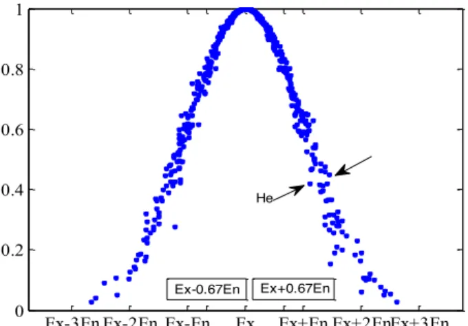
is a measurement of the uncertainty of entropy-En. The larger the value of He, the more random the set of membership degrees is distributed. Figure 1 shows the three numerical characteristics of the cloud model.

Through statistical analysis, the cloud drops that contribute to qualitative concept-C in universe-U, are within interval [Ex-3En, Ex+3En], and the contribution rate is 99.74%. The cloud drops within interval [Ex-0.67En,

Ex+0.67En] account for 22.33% of the total quantitative numerical, and the contribution rate is 50%. These cloud drops are called the “backbone element”; the cloud drops within interval [Ex-En, Ex+En] account for 34.33% of the total quantitative numerical, and the contribution rate is 68.26%. These cloud drops are called the “basic element”; the cloud drops within interval [Ex-3En, Ex-2En] and [Ex+2En, Ex+3En] account for 34.33% of the total

quantitative numerical, and the contribution rate is 27.18%. These cloud drops are called the “peripheral element”; the cloud drops within interval [Ex-2En, Ex-En] and [Ex+En,

Ex+2En] account for 34.33% of the total quantitative numerical, and the contribution rate is 4.3%. These cloud drops are called the “weak peripheral element”. The contribution of cloud drops in different regions to the qualitative concept is shown in Figure 1.

2.2 Cloud probability distribution density

Suppose Ln = {l1, l2, …, ln}are the cloud drops of samples-W to concept-T in universe-L. Samples-W comes from the parent population-Ω, and n is the sample size, f(l) is the probability density function of parent

population-Ω.WSuppose x=φ(l-li), (i=1,2,…,n). There is a Borel

measurable function within( ‐∞, + )∞ , which represents stochastic membership conception T of x, as is denoted by

CT(x). The membership conception-T’s data energy of li can

be radiated to l. Suppose

t

i

=

“around of li”, and the initial

distribution of radiated cloud drops can be expressed by Q x( )=∑C xT( )=∑C g l lT( ( −i)) . CT(x) is a radiation

brightness function for conception-T in universe-L.

( i) / , 0

x₌ l₋l d d_> can be deduced from x=φ(l-li), in which

d is called radiation unit, and formula (1) is deduced to be[9]:

1 1

1 1

ˆ ( ) ( ) ( )

n n

i

T T

i i

l l

f l C x C

n = nd = d

−

=

_∑

=

_∑

₍₁₎

From formula (1) we can see that the cloud probability distribution density is an estimation of the parent cloud model according to data radiation. CT(x) and d are keys to

radiation estimation. It is important to obtain an appropriate radiation brightness function and the radiation unit through sample-W. Cloud drops radiation takes into consideration randomness and fuzziness at the same time, selects the radiation spot of the data energy as the kernel, and redistributes the total radiation brightness of the sample-W.

Thus, new membership sets Q(x)={ Q1/nd, Q2/nd,…,Qn/nd} of concept-T have taken shape. It is a random distribution in the basic universe-L by the cloud drops radiation. When

( i) /

x= l−l d, then Qn/nd is the kernel estimation (Parzen, 1962). According to formula (1), the probability density of cloud drops can be estimated based on the data radiation energy of cloud drops. In contrast, the initial concept sets can be established from the probability density function of spatial data distribution through cloud transformation. Obviously, it is an inverse cloud process. Data radiation provides an inverse explanation for cloud transformation from the perspective of physics.

The derivative of the radiation brightness function can be expressed as:

0 0

0

0 0

( ) ( )

( )

( ) lim T lim T T

T

x x

C x x C x

C x

C x

x x

Δ → Δ →

+Δ − Δ

′ = =

Δ Δ

(2)

Which is shown in Figure 2.

The radiation brightness function CT(x) must match the

constraint condition [10]:

1

0 ( )

2

T

C x

πσ

≤ ≤ (3)

Ex-3En Ex-2En Ex-En Ex Ex+En Ex+2EnEx+3En 0

0.2 0.4 0.6 0.8 1

He

Ex-0.67En Ex+0.67En

( ) ( ) 1

T T

R

C x dx C x dx

+∞

−∞ = =

∫

∫

(4)

| |

lim

x T

( )

0

xC

x

→∞

=

(5)

( ) 0

T R

xC x dx=

∫

(6)

2 2

( )

T R

x C x dx=

_σ

∫

(7)

2 1

( ) 2

T R

C x dx

πσ

=

∫

(8)

According to formulae (3) ~ (8), another characteristic of the radiation brightness function can be demonstrated.

Suppose liis an independent random observation in data

space-R, the expectation of formula (1) can be expressed as:

1 1

ˆ ( ) ( ) ( ) ( )

1

( ) ( )

i

n T T

i i R

T n R

l l l x

Ef l EC C f x dx

nd d nd d

l x

C f l x dx

d d − − = = − = −

∑

∑ ∫

∫

(9) 1

ˆ ( ) ( ) ( ( ) ( )) ( )

( ) ( ) ( )

T R

R R

l x

Ef l f l f l x f l C dx

d d

A x dx A x dx A x dx

η −η

− − = − − = ≤ +

∫

∫

∫

∫

(10)

In formula (10), η is a neighborhood of 0. If η→0, then

( )

n

A x dx

∫

→arbitrarily small, which can be addressed as O1,

then

1

1

1 2 3

1

ˆ ( ) ( ) ( ) ( )

1

( ) ( )

1

sup ( ) ( ) ( ) ( )

T R T R T T R R x Ef l f l O f l x C dx

d d

x

f l C dx

d d

x x x

O C f x dx f l C dx

d d d d

O O O

η η η − − − − ≤ + − + ≤ + + ≤ + +

∫

∫

∫

∫

(11)

If η→∞, then

d η

→ ∞. After that, according to formula

(5), O2→0 can be obtained. Finally, 3 T( ) R

d

O C x dx

η − =

_∫

_, lim n R d η →∞ →

, and based on formula (4), O3→0 can be obtained.

So _lim ˆ_{( ) ( )}

n→∞Ef l =f l can be demonstrated.

2.3 Radiation unit and best radiation unit

According to formula (1) and formula (10), the evaluationf lˆ ( )of the parent population’s probability density function depends on the radiation unit d, the monitoring value li and the number n of monitoring value (sample size).

After the observation, the monitoring value of li and the

number of n are known, but radiation unit d is unknown. So

d must be decided firstly. Suppose E is the expectation, and

D is the variance, according to formula (4) and formula (5), the variance of CT(x) can be obtained:

1

2 2 2

2

1 1

2

2 1 1 2 2 1

2 2 2 2 2 2 1 1

ˆ ( ) ( ) ( )

1 ( ) ( ) 1 1 ( ) ( ( )) ( ) 1 ( ) ( ) 1 ( / ) ( ) i T T i T T

T T T

T R

T R

l l l l

Df l DC DC

n d d nd d

l l l l

E C EC

nd d d

l l l l l l

EC EC EC

nd d d nd d

l x

C f x dx

nd d

C x d f l x dx

nd − − = = − −   = _ − _   − − −   = _ − _≤   − = = −

∑

∫

∫

(12) ˆ lim ( ) 0

x→∞Df l =

(13)

Suppose 2

( ) 0, ( )

T T

R R

xC x dx₌ k₌ x C x dx_<∞

∫

∫

, then

2 2

2

1 _ˆ 1

( ( ) ( )) ( )( ( ) ( )) 1 ( ) ( ) T R T R

Ef l f l C x f l xd f l dx

d d

f l xC x dx d − = − − ′ +

∫

∫

(14)

Suppose η ≤₁, and according to the mean value

theorem, 2

1 _ˆ

(Ef l( ) f l( ))

d − can be expressed as:

2 2

2

1 _ˆ ( ) ( ) ( )

( ( ) ( )) ( ) 1 ( ) ( ) 2 T R T R

f l xd xdf l f l

Ef l f l C x

d d

C x x f l ηxd dx

′ − + − − = ′′ = −

∫

∫

(15)

/Journal of Engineering Science and Technology Review 7 (3) (2014) 82 – 89 According to the dominated convergence theory, if

( ) 0

f l′′ ≠ , O is the infinitesimal of higher order, then

2 2

1

ˆ ( ) ( ) ( ) ( ) 2

Ef l −f l = f l kd′′ +O d (16)

The mean square error is:

2

2 2 2 2

ˆ ˆ ˆ

( ( )) ( ) ( ( ) ( ))

1 ( ( ) )

( ) ( )

4 ( )

T R

MSE f l Df l Ef l f l

f l k d

f l C x dx O

nd

A d O

= + −

′′

= + +

= +

∫

(17)

From formula (17) we can see that the value of radiation unit is the key factor, and it is essential to obtain the appropriate radiation unit through sample W.

The best radiation unit is defined as a unit with the minimum mean square error. According to formula (17), the main part A(d) of mean square error is a function of d. Suppose the derivative of A(d) is 0, then:

2 2 2 3

2 ( )

( ) ( ( )) 0

T R f l

C x dx f x k d dx

nd ′′

−

_∫

+ =

(18)

And there is:

2 5 2 2 ( ) ( ) ( ( )) T R

f l C x dx d

n f x k

=− ′′

∫

₍₁₉₎

Substitute formula (19) into formula (17), formula (20) is expressed by:

(

)

2 _0.8

2 0.4

0.8 0.8

5 ( ) 1

ˆ

( ( )) ( ) [ ( )] ( )

4 R T

f l

MSE f l C x dx kf l O

n ′′ n

=

_∫

+ (20)

Suppose 2 2 2 1 ( ) 2 l

f l e σ

πσ −

= , then:

2 2

0.2

9

2 2 2 2

( )

2 ( )

l

d l

n l e σ

σ σ σ −     =_{ } ≠±  ₋    (21)

However, f(l) is unknown in the real situation. So the best radiation unit cannot be worked out from formula (15). According to the properties of radiation brightness function- CT(x), when n→maximum, there is f l( )_i ≈f lˆ( )_i .

As

0

( ) ( )

( ) lim

h

f l d f l

f l d → + − ′ = , 2 0

( ) 2 ( ) ( )

( ) lim h

f l d f l f l d

f l

d

→

+ − + −

′′ = , lim n 0

n

d

→∞ = , Suppose

radiation unit is d, and get rid of the sign of limits, there is:

2

ˆ_{( ) 2 ( )}ˆ ˆ_{( )}

( ) i i i

i

f l d f l f l d

f l

d

+ − + −

′′ = (22)

Substitute f l( )_i ≈ f lˆ( )_i and formula (20) into formula (19), and the iteration computational equations of radiation unit can be worked out.

0 0.2 4 1 2 1 1 1

(max( ) min( )) / ( 1)

ˆ 0.26833 ( )( )

ˆ ˆ ˆ

[ ( ) 2 ( ) ( )]

( ) 1

ˆ _{( ) ( )}

j j

j i

i _{j j j j j}

i i i

j j i j i T j j i

d l l n

f l h d

n f l d f l f l d

d median

l l

f l C

nd d + + + +  = − −       =_{  }  + − + −    _{ }  =  − _ = 

∑

(23)

2.4 The best radiation brightness function

The best radiation brightness function can be determined by the best radiation unit.

Suppose 2 2

( T ( ) )

R

k

_∫

C x dx → minimum, there is:

2

3

(5 ) 5

20 5 ( ) 0 5 T x x C x x

 _{− <}



=_

 _≥



(24)

2.5 The cloud numerical characteristics based on data radiation

On the basis of a normal cloud generator and a backward cloud generator, the mapping relationship between qualitative and quantitative can be established through three numerical characteristics: Expectation (Ex), Entropy (En) and Hyper Entropy (He). In the process of qualitative and quantitative transformation through the cloud model, it is important to consider the premises of using cloud probability density that is in line with the data. Each cloud drop radiates the data energy for a concept in the number field space. Thus, all the cloud drops distribution obeys a certain probability density distribution on the whole. From the perspective of radiation data, cloud numerical characteristics must be closely related to the probability density of cloud drops, and the probability density of it should not be overlooked. Otherwise, we cannot get the parent population cloud. The algorithm of cloud numerical characteristics is described as follows.

First, estimate the probability density of cloud drops based on data radiation. Second, use the probability density of cloud drops to measure the weight of each sample of cloud drops to the parent population. Finally, according to the weighted average algorithm of spatial distribution, calculate the three numerical characteristics (Expectation (Ex), Entropy (En) and Hyper Entropy (He):

1

1

ˆ ( ) ˆ ( )

ˆ ( )

n i i i n i i

1 1

ˆ_{( )(} ˆ ₎ ˆ ( )

ˆ ( )

n i i i n i i

f l l Ex En l f l = = − =

∑

∑

(26) 2 1 1 ˆ ˆ [ ( ( ))( ( ) ( ( ))] ˆ ( )

ˆ ( ( ))

n

i i i

i

n

i i

f En l En l En En l

He l

f En l

= = − =

∑

∑

(27)

From formula (25) ~ formula (27) we know that the algorithm fits the spatial distribution characteristics of cloud drops. The algorithm is easy to understand and is superior to the arithmetic average method.

2.6 Cloud expectation function based on data radiation The cloud expectation function is the probability density function of the spatial entities’ parent population. It is also the mathematical expectation function of cloud drops that are in line with the sample of spatial data. So the cloud expectation function can be acquired by the probability density of cloud drops. The cloud expectation function is:

2 2

ˆ ˆ

[ ( )( )] 2[ ( )] 1

( ) ˆ ( )

f l l Ex En l T

C l e

f l

− −

= ₍₂₈₎

If the probability density of cloud drops is equal anywhere in the number field space, thenf lˆ ( ) 1= , and the cloud expectation function is the same as the function

2 2 ˆ ( ) 2( ) ( ) lEx En T

C l e

− −

= of the normal cloud model.

According to the cloud expectation function, the three numerical characteristics of the cloud model are acquired from the given data by using the cloud generator. Based on this, it is possible to describe the morphological characters of the cloud model. So the cloud radiation expectation function is in line with the backward cloud generator.

2.7 cloud radiation algorithm

The cloud radiation algorithm is based on the backward cloud generator, which is an uncertainty transformation model realizing the transformation between a numeric value and its linguistic value. It effectively converts a certain number of accurate data to the concept indicated by appropriate qualitative linguistic values {Ex, En, He} which are the characteristics of the whole drops. Based on the data radiation, a new improved algorithm of backward cloud generator is described as follows [11]:

Input: Coordinate value li of each cloud drops and its

degrees of certainty-CT(li);

Output: Ex, En and He, cloud drops’ number N;

• Fit the cloud expectation curve

2

2 ˆ ˆ [ ( )( )]

2[ ( )] 1

( ) ˆ ( )

f l l Ex En l T

C l e

f l

− −

= of cloud drops, and get

1

1 ˆ ( ) ˆ ( )

ˆ ( )

n i i i n i i

f l l Ex l f l = = =

∑

∑

which is the estimation value of

Ex;

• Eliminate the dots that fit the condition of

CT(l)>0.999, andthere are m cloud drops left;

• Calculate

ˆ ( )( ) ˆ ( )

2 ln( ( ) ( ))

i i

i

i T i

f l l Ex En l

f l C l −

=

− ;

• Calculate the estimation value of En:

• 1

1

ˆ

[ ( ( )) ( )] ˆ ( )

ˆ [ ( ( )) m i i i m i i

f En l En l En l

f En l

= = =

∑

∑

;

• Calculate the estimation value of He:

• 2 1 1 ˆ ˆ [ ( ( ))( ( ) ( ( ))] ˆ ( )

ˆ ( ( ))

n

i i i

i

n

i i

f En l En l En En l He l

f En l

= = − =

∑

∑

.

3. Analysis of observation data based on cloud probability distribution density algorithm

Luhun reservoir is an earth-rockfill dam in Luoyang, China. 13 piezometric tubes of Luhun reservoir were selected for the purposes of calculation. Piezometric tubes S1~S9 were embedded in the body of the dam and piezometric tubes D2~D5 were embedded in the fault zone of the dam’s foundation. Piezometric tubes S1, S4 and S7 were embedded in section 1 (0+813); piezometric tubes S2, S5 and S8 were embedded in section 2 (0+660); piezometric tubes S3, S6 and S9 were embedded in section 3 (0+540); piezometric tubes D2 and D4 were embedded in section 5 (0+640); piezometric tubes D3 and D5 were embedded in section 6 (0+680).See Figure 3.

The probability distribution density of the piezometric tubes’ water levels between 1979~1999 were acquired, and the results are shown in figure 4~ figure 16, in which the vertical axis represents probability density estimation and the horizontal axis represents water level value. The qualitative linguistic values (three numerical characteristics {Ex, En, He}) are used to describe the monitoring results, which can be obtained through the improved backward

/Journal of Engineering Science and Technology Review 7 (3) (2014) 82 – 89 cloud generator algorithm. The three numerical

characteristics {Ex, En, He} are shown in Table I.

According to the qualitative explanatory rules, Ex refers to the water level of a piezometric tube; En refers to the dispersion degree between water level and expected water level of a piezometric tube; He refers to the influence of monitoring instruments and monitoring environment on monitoring level. From figure 4~ figure 16 and Table 1 we can see that the saturation line of Section 1 is the highest, the saturation line of Section 2 is the second, the saturation line of Section 3 is the lowest, the saturation line of each section is not high and in a stable state; all the piezometric tubes’ dispersion degree of each section are in a low state and the maximum value (En) is less than 1. The maximum value (He) of piezometric tube in each section is 0.13, which indicates that the monitoring level is stable.

Tab.1. Numerical characteristics of piezometric tubes’ water level

Location Section Piezometric

tube Ex En He

In the body of the dam

Section 1

S1 276.12 0.49 0.13

S4 276.11 0.47 0.11

S7 276.07 0.5 0.13

Section 2

S2 276.11 0.42 0.07

S5 276.03 0.47 0.11

S8 276.02 0.46 0.07

Section 3

S3 276.01 0.44 0.11

S6 276.01 0.45 0.08

S9 276.01 0.43 0.08

In the fault zone

Section 4 D2 275.77 0.83 8.1

D4 275.96 0.44 0.09

Section 5 D3 276.00 0.44 0.09

D5 276.05 0.46 0.13

The water level of the piezometric tubes in section 4 and section 5 is lower than that in the body of the dam. The water levels are in a stable state except in piezometric tube D2. The entropy (En) of piezometric tube D2 is 0.83, and the hyper entropy (He) of piezometric tube D2 is 8.1. This means that there are some problems about the dispersion degree and the monitoring level is affected by monitoring

instruments and the monitoring environment. So piezometric tube D2 needs to be studied further and treated in the fault zone.

Fig. 7. Probability density of S2 Fig. 6. Probability density of S7

Fig. 5. Probability density of S4

Fig. 13. Probability density of D2 Fig. 12. Probability density of S9 Fig. 11. Probability density of S6

/Journal of Engineering Science and Technology Review 7 (3) (2014) 82 – 89

4. Conclusions

This paper proposes an improved algorithm of cloud probability density based on a backward cloud generator and applies it to the analysis of monitoring data of piezometric tube water levels in an earth-rockfill dam. The corresponding cloud probability density distribution map and cloud numerical characteristics are demonstrated and serve to monitor the seepage of the dam. The results show that most of the tubes are in a stable state. Only D2 presents excessive entropy and hyper entropy, which may be caused by a change in seepage or outdated equipment, but which needs further inspection.

However, the algorithm still has the following loopholes. First, due to limited space, this paper fails to consider the special distribution of data. So the influence of location uncertainty on the monitoring of the parent population has been overlooked. Second, this paper assumes that the monitoring data are in line with Gaussian distribution, which requires further proof and research.

Acknowledgments

The authors wish to thank Natural Science Fund Committee (51279064 and U1304511) and the editor of the journal.

______________________________ References

1. Rohaninejad, Mohsen, Bagherpour, Morteza, “Application of risk analysis within value management: A case study in dam engineering”. Journal of Civil Engineering and Management, 19(3), 2013, pp. 364-374.

2. Zhenjun Wu, Wang Shuilin, Ge Xiurun, “Slope reliability analysis by random FEM under constraint random field”. Rock and Soil Mechanics, 30(10), 2009, pp. 3086-3092.

3. Li Dianqing, Qi Xiaohui, Zhou Chuangbing, Zhang Limin. “Reliability analysis of infinite soil slopes considering spatial variability of soil parameters”. Chinese Journal of Geotechnical Engineering, 35(10), 2013, pp. 1799-1806.

4. Erfeng Zhao, Kai Zhu, Jiangyang Liu. “Random dynamical model for mechanical time-varying characteristics of gravity dam foundation”. Engineering Journal of Wuhan University, 46(1), 2013, pp. 89-94.

5. Altunok Erdogan, Taha Mahmoud M. Reda, Epp David S, Mayes Randy L, Baca Thomas J, “Damage pattern recognition for structural health monitoring using fuzzy similarity prescription”. Computer-Aided Civil and Infrastructure Engineering, 21(8), 2006, pp. 549-560.

6. Cui Shaoying, Bao Tengfei, Pei Yaoyao, Chen Shanying, “Data processing of dam safety monitoring based on fuzzy mathematical approach”, Water Resources and Power, 30(10), 2012, pp. 45-48. 7. Yanjun Long, Jianquan Ouyang, Xinwen Sun, “Network Intrusion

Detection Model based on Fuzzy Support Vector Machine”, Journal of Networks, 8(6), 2013, pp. 1387-1394.

8. Li Deyi, Du Yi, Artificial intelligence with uncertainty, Beijing: National defense industry press, 2005, pp.137-182.

9. Wang. Shuliang, “Data Field and Cloud Model Based Spatial Data Mining and Knowledge”, Thesis ofWuhan University, 2002, pp.83-117.

10. Shannon, C., Weaver,W., Mathematical theory of communication, Illinois: University of Illinois Press, 1949, pp.158-178.

11. Li Deren, Wang Shuliang, Li Deyi, Spatial data mining theories and applications, Beijing: Science press, 2006, pp.425-470. Fig. 16. Probability density of S1