www.atmos-chem-phys.net/16/6805/2016/ doi:10.5194/acp-16-6805-2016
© Author(s) 2016. CC Attribution 3.0 License.
Near-surface and columnar measurements with a micro pulse lidar
of atmospheric pollen in Barcelona, Spain
Michaël Sicard1,2, Rebeca Izquierdo3, Marta Alarcón3, Jordina Belmonte4,5, Adolfo Comerón1, and José Maria Baldasano6,7
1Remote Sensing Laboratory, Universitat Politècnica de Catalunya, Barcelona, Spain
2Ciències i Tecnologies de l’Espai – Centre de Recerca de l’Aeronàutica i de l’Espai/Institut d’Estudis Espacials de Catalunya
(CTE-CRAE/IEEC), Universitat Politècnica de Catalunya, Barcelona, Spain
3Departament de Física, Universitat Politècnica de Catalunya (UPC), c/Urgell 187, 08036 Barcelona, Spain
4Departament de Biologia Animal, Biologia Vegetal i Ecologia, Universitat Autònoma de Barcelona (UAB). Edifici C,
08193 Bellaterra, Spain
5Institut de Ciencia i Tecnología Ambientals (ICTA), Universitat Autònoma de Barcelona (UAB), Edifici Z,
08193 Bellaterra, Spain
6Earth Sciences Department, Barcelona Supercomputing Center – Centro Nacional de Supercomputación, Barcelona, Spain 7Environmental Modeling Laboratory, Technical University of Catalonia, Barcelona, Spain
Correspondence to:Michaël Sicard (msicard@tsc.upc.edu)
Received: 11 March 2016 – Published in Atmos. Chem. Phys. Discuss.: 16 March 2016 Revised: 18 May 2016 – Accepted: 21 May 2016 – Published: 6 June 2016
Abstract. We present for the first time continuous hourly measurements of pollen near-surface concentration and lidar-derived profiles of particle backscatter coefficients and of volume and particle depolarization ratios during a 5-day pol-lination event observed in Barcelona, Spain, between 27 and 31 March 2015. Daily average concentrations ranged from 1082 to 2830 pollen m−3. Platanus andPinuspollen types
represented together more than 80 % of the total pollen. Max-imum hourly pollen concentrations of 4700 and 1200 m−3
were found forPlatanusandPinus, respectively. Every day a clear diurnal cycle caused by the vertical transport of the airborne pollen was visible on the lidar-derived profiles with maxima usually reached between 12:00 and 15:00 UT. A method based on the lidar polarization capabilities was used to retrieve the contribution of the pollen to the total aerosol optical depth (AOD). On average the diurnal (09:00– 17:00 UT) pollen AOD was 0.05, which represented 29 % of the total AOD. Maximum values of the pollen AOD and its contribution to the total AOD reached 0.12 and 78 %, respec-tively. The diurnal means of the volume and particle depolar-ization ratios in the pollen plume were 0.08 and 0.14, with hourly maxima of 0.18 and 0.33, respectively. The diurnal mean of the height of the pollen plume was found at 1.24 km
with maxima varying in the range of 1.47–1.78 km. A corre-lation study is performed (1) between the depolarization ra-tios and the pollen near-surface concentration to evaluate the ability of the former parameter to monitor pollen release and (2) between the depolarization ratios as well as pollen AOD and surface downward solar fluxes, which cause the atspheric turbulences responsible for the particle vertical mo-tion, to examine the dependency of the depolarization ratios and the pollen AOD upon solar fluxes. For the volume depo-larization ratio the first correlation study yields to correlation coefficients ranging 0.00–0.81 and the second to correlation coefficients ranging 0.49–0.86.
1 Introduction
wa-ter stress (Dahl et al., 2013). Pollen is primarily dispersed in the atmosphere by insects or wind. Wind-pollinated plants are called anemophilous and they produce huge amounts of pollen grains which, once airborne, are responsible of al-lergenic reactions when inhaled by humans (Cecchi, 2013). Fungal spores are a biological component that can be found any time of the year in the atmosphere (Lacey, 1981; Burch and Levetin, 2002). Environmental variables, such as temper-ature and moisture, can influence growth and reproduction in fungi which makes airborne spore concentrations to fluctu-ate seasonally (Grinn-Gofrón and Strzelczak, 2008; Pakpour et al., 2015). However, it has also been observed that local climate, vegetation patterns, and management of landscape are governing parameters for the overall spore concentration, while the annual variations caused by weather, although not negligible, are of secondary importance (Skjøth et al., 2016). Fungi are, after pollen, the second most important producers of outdoor airborne allergens (Weikl et al., 2015). Their pres-ence can cause human health problems (mainly allergies) and crop infections (phytopathology) (e.g., Burge and Rogers, 2000; Simon-Nobbe et al., 2008). Up to 80 % of asthmat-ics are sensitized to fungal allergens (Lopez and Salvaggio, 1985) and a disease pattern of severe asthma with fungal sen-sitization has been recently proposed (Denning et al., 2006). Worldwide many people living in large cities suffer from allergies linked to the presence of atmospheric pollen and fungal spores. In the industrialized countries of central and northern Europe, up to 15 % of the population is sensi-tive to pollen allergens (WHO, 2003; Cecchi, 2013). In Eu-rope the most common types of pollen are Ambrosia, Al-nus, Artemisia, Betula, Corylus, Chenopodiaceae, Cupres-saceae/Taxaceae,Olea,Platanus, Poaceae,Quercus, and Ur-tica/Parietaria (Skjøth et al., 2013). Although their con-centration is monitored daily at ground level by aerobio-logical networks (Scheifinger et al., 2013; Karatzas et al., 2013), very little is known on their vertical distribution and their long/short-range transport (Sofiev et al., 2013) al-though an increase in interest has arisen very recently in the aerosol lidar community (Sassen, 2008; Noh et al., 2013a, b). Sassen (2008) reported on lidar measurements in the lower atmosphere of birch pollen plumes from the boreal forest of Alaska. Noh et al. (2013a) retrieved optical properties with a polarization-sensitive lidar forPinusandQuercuspollen in South Korea. Noh et al. (2013b) reported on the vertical dis-tribution of the same pollen event observed with lidar and on the dependency of its diurnal variations upon the meteoro-logical conditions (temperature, relative humidity, and wind speed). Sugimoto et al. (2012) developed a lidar spectrometer system with high spectral resolution which showed promis-ing results for investigatpromis-ing the vertical structure of biologi-cal particles.
In the Mediterranean city of Barcelona, Spain, the most abundant pollen taxa areQuercus(27.4 % of the total pollen), Pinus, Platanus, Cupressaceae,Olea, Urticaceae, Poaceae, Chenopodiaceae,Plantago, Moraceae,Fraxinus, Castanea,
andPopulus(1 %) according to the Aerobiological Network of Catalonia (http://lap.uab.cat/aerobiologia) and based on pollen concentrations measured in the period 1994–2015. Barcelona is the Spanish city which presents the longest mean pollen season of Platanus pollen. Maximum daily counts occur generally during the second half of March (Díaz de la Guardia et al., 1999).Platanus hispanicais responsible of the most frequent pollen sensitizations (37 %) detected in Barcelona (Puiggròs et al., 2015).Pinusis one of the most abundant pollen taxa in Spain (Belmonte and Roure, 1991; De Linares et al., 2014). In Barcelona,Pinuspollination oc-curs in two phases: the most important one happens from March to May and the other in June–July. Regarding airborne fungal spores,Cladosporiumis the most abundant taxon in Barcelona, representing up to 44 % of the total fungal spore spectrum. It is present all year round and shows the high-est concentrations in April–May and November (Infante et al., 1999; see also http://lap.uab.cat/aerobiologia). This pa-per aims at investigating the possible correlation between pollen near-surface concentration and columnar properties measured during a 5-day pollination event in Barcelona. The data set is composed of continuous measurements at a tem-poral resolution of 1 h. The influence of the meteorological conditions and the solar radiation on the pollen dispersion is also investigated. This contribution relates for the first time near-surface and lidar measurements of pollen in a large Eu-ropean city.
The paper is organized as follows: Sect. 2 presents the methods used to count the pollen and spore taxa and also de-scribes the lidar instrument used and the method employed to estimate the pollen optical properties. Pollen and spores mea-sured in Barcelona are first analyzed with daily mean concen-tration values and lidar quick looks (time–altitude contour plots) in Sect. 3. The analysis of the temporal evolution of hourly concentrations and meteorological parameters com-pletes this section. Section 4 is dedicated to the investigation of possible correlations between near-surface pollen concen-tration and the vertical distribution of a series of structural and optical properties. Finally Sect. 5 enlightens us on the relationship between the vertical transport of airborne pollen and the solar radiation.
2 Instrumentation and method
2.1 Pollen and spores sampling instrumentation, PM10,
and meteorological data
han-dle a flow of 10 L of air per minute, thus matching the human breathing rate. Pollen and spores are impacted on a cylin-drical drum covered by a Melinex film coated with a 2 % silicon solution as trapping surface. The drum was changed weekly and the exposed tape was cut into seven pieces, each one corresponding to 1 day, which were mounted on separate glass slides. Pollen and spores were counted under a light microscope at 600X magnification. Daily average pollen and spore counts were obtained following the standardized Span-ish method (Galán Soldevilla et al., 2007), consisting in run-ning four longitudinal sweeps along the 24 h slide for daily data, identifying and counting each pollen and spore type found. To obtain the hourly concentrations, 24 continuous transversal sweeps separated every 2 mm along the daily-sample slide were analyzed, since the drum rotates at a speed of 2 mm h−1. Daily and intra-diurnal (hourly) pollen and spore concentrations are obtained converting the pollen and spore counts into particles per cubic meter of air, taking into account the proportion of the sample surface analyzed and the air intake of the Hirst pollen trap (10 L min−1).
PM10measurements were acquired at the “Eixample” sta-tion of the Xarxa de Vigilància i Previsió de la Qualitat de l’Aire (XVPCA, the Catalonian network for monitoring and forecasting the air quality). It is located at 1.2 km to the southwest of the pollen sampling instrumentation.
Meteorological data were recorded in the “Zona Univer-sitaria” area of Barcelona, at approximately 0.6 km south-southeast of the lidar site.
2.2 The Barcelona Micro Pulse Lidar (MPL)
The profiles of the particle backscatter coefficient and the particle depolarization ratio were measured with the Barcelona MPL system, model MPL-4B. The system is lo-cated in the “Zona Universitaria” area of the city, on the roof of the Remote Sensing Lab (RSLab) building in the North Campus of the Universitat Politècnica de Catalunya (2.112◦E, 41.389◦N; 115 m a.s.l.), approximately 1 km from Sierra de Collserola and 7 km from the sea. It is located at 4.4 km to the west of the pollen sampling instrumentation. The system should become very shortly part of the MPLNET (Micro Pulse Lidar Network, http://mplnet.gsfc.nasa.gov/) network. The MPL system is a compact, eye-safe lidar de-signed for full-time unattended operation (Spinhirne, 1993; Campbell et al., 2002; Flynn et al., 2007; Huang et al., 2010). It uses a pulsed solid-state laser emitting low laser pulse en-ergy (∼6µJ) at a high pulse rate (2500 Hz) and a co-axial
“transceiver” design with a telescope shared by both transmit and receive optics. The Barcelona MPL optical layout uses an actively controlled liquid crystal retarder which makes the system capable to conduct polarization-sensitive measure-ments by alternating between two retardation states (Flynn et al., 2007). The signals acquired in each of these states are recorded separately and called “co-polar” and “cross-polar”.
In nominal operation the raw temporal and vertical resolu-tions are 30 s and 15 m, respectively.
The linear volume depolarization ratio,δV, is defined as
δV(z)=β⊥(z) β||(z)
=P⊥(z)
P||(z)
, (1)
where β− and β|| denote the total (particles+molecules) perpendicular and parallel backscatter coefficient, respec-tively, andP−andP||represent the perpendicular and paral-lel backscatter powers, respectively. According to Gimmes-tad (2008)δVcan also be expressed as a function of a factor d, which has a range of 0–1 and is related to the propensity of
the scattering medium to preserve the incident polarization:
δV(z)= d
2−d. (2)
In the case of a linear polarization lidar,d=0 indicates that
no depolarization occurs, whiled=1 indicates that the
re-turned beam is completely depolarized. By adapting the no-tations of Flynn et al. (2007), especially in Eqs. (1.4) and (1.6), one can formulate the linear volume depolarization ra-tio for the MPL system as
δV(z)= Pcr(z)
Pco(z)+Pcr(z), (3)
wherePcr andPco represent the MPL cross- and co-polar
channels, respectively.
The linear particle depolarization ratio,δp, can then be
de-termined by (Freudenthaler et al., 2009)
δp(z)=β
p
⊥(z)
β||p(z)
=
1+δmδV(z)R(z)−1+δV(z)δm
[1+δm]R(z)−1+δV(z) , (4)
whereβ⊥p andβ||p are the particle perpendicular and
paral-lel backscatter coefficients, respectively,δmis the molecular
depolarization ratio andR is the backscatter ratio, which is
defined as
R(z)=β
m(z)+βp(z)
βm(z) , (5)
where βm and βp denote the molecular and particle
backscatter coefficient, respectively, of the total (perpendic-ular+parallel) returned signal. According to the MPL
opti-cal requirements in the receiving system the spectral filter-ing is performed by filters with a spectral band≤0.2 nm.
This number produces a temperature-independent molecular depolarization ratio ofδm=0.00363 according to Behrendt
and Nakamura (2002).
The particle backscatter coefficient,βp, was retrieved with
Nakane, 1984; Klett, 1985) with a constant lidar ratio of 50 sr and applied to the total lidar signal,P, reconstructed from the
MPL lidar signals as (Flynn et al., 2007)
P (z)=Pco(z)+2Pcr(z). (6)
The value of 50 sr is motivated by two previous studies. First, it falls in the range of the mean columnar lidar ra-tios, 46–69 sr, found in Barcelona during the period from February to April and calculated over a period of 3 years (Sicard et al., 2011). In that work the columnar lidar ratio was retrieved with the two-component elastic lidar inversion algorithm constrained with the aerosol optical depth (AOD) from a sun photometer (Landulfo et al., 2003; Reba et al., 2010). Second, Noh et al. (2013b) used the same method and found a mean columnar lidar ratio of 50±6 sr during a 6-day
pollination event (mostly dominated byPinusandQuercus pollen) in South Korea. At the peak of the event the pollen AOD represented up to 35 % of the total AOD.
2.3 Determination of pollen optical and structural properties
Pollen has formerly been distinguished from other particle types thanks to its depolarization capabilities (Sassen, 2008; Noh et al., 2013a, b). Although many types of pollen have regular shapes (circular, spherical, elliptical, ovoid, etc.), they cannot be considered spherical from the point of view of light scattering because they do not generate Mie patterns expected from a sphere of equivalent size. The reason lies in surface imperfections of pollen grains and inhomogeneous refractive indices inside the grains
When the atmospheric particle load can be assumed as the external mixing of one type of depolarizing particles (here, the pollen) with another type of much less depolarizing par-ticles, the method suggested by Shimizu et al. (2004) allows us to separate the contribution ratio of both types of parti-cles. The same rationale leading to Eq. (4) allows us to define a pollen (highly depolarizing particles) contribution ratio to the total particle depolarization ratio, CRpol, expressed as
CRpol(z)=
δp(z)−δno-pol 1+δpol
δpol−δno-pol[1
+δp(z)], (7)
where δno-pol andδpolare the particle depolarization ratios
of all particle types except pollen (weakly depolarizing) and of only the pollen (depolarizing), respectively. One can check easily whether no pollen is present (δp=δno-poland
Eq. (7) leads to CRpol=0) and whether only pollen is present
(δp=δpoland Eq. (7) leads then to CRpol=1). The pollen
backscatter coefficient,βpol, is simply calculated as
βpol(z)=CRpol(z)βp(z). (8)
The contribution ratio is sensitive to the selection ofδno-pol
and δpol, which are determined either empirically or taken
from references. To fix the value ofδno-polwe searched for
a clear-sky day prior to the pollination event without long-range transport aerosols. Such conditions were fulfilled on 15 March around 12:00 UT. On that day a well-mixed atmo-spheric boundary layer (ABL) developed. At 12:00 UT the ABL height was∼1.2 km and the AOD 0.18. The particle
depolarization ratio was constantly∼0.03 in the whole ABL.
We have takenδno-pol=0.03. In the literature very few
infor-mation on measurements of pollen depolarization ratios is available. The choice ofδpolis deferred to Sect. 4, after the
analysis of the individual profiles ofδp, in order to have as
much information as possible. A short discussion on the un-certainty of CRpolandβpollinked to the choice ofδpolis also
discussed in Sect. 4.
Finally we also calculated the vertical height,hpol, up to
which the pollen plume extends. As it is shown in Sect. 4, the pollen plume is characterized during the whole polli-nation event by a near-constant or slightly decreasing pro-file of βpol. From this aspect the structure of the pollen
plume is much simpler than the ABL structure usually found in Barcelona (Sicard et al., 2006). This allows us to use a simple threshold method such as the one used to esti-mate the ABL height by Melfi et al. (1985) and Boers et al. (1988). After several tests we empirically set a threshold of 0.055 Mm−1sr−1and definedhpolas the height at which βpol(z) <0.055 Mm−1sr−1. This empirical threshold
guar-antees that the integral ofβpol(z)up tohpolrepresents at least
99 % of its integral over the whole atmospheric column.
3 Temporal variation of pollen and spore taxa near-surface and columnar properties
In the second half of March 2015 a strong anticyclone posi-tioned in the Atlantic Ocean west of the Portuguese coast generated northwesterly winds in the northeastern part of the Iberian Peninsula. In Barcelona, the synoptic condi-tions resulted in marked, off-shore winds in altitude yield-ing to relatively clear skies and preventyield-ing long-range trans-port of highly depolarizing aerosols like mineral dust over Barcelona. To confirm that mineral dust was not transported over Barcelona during the pollination event, we used the dust transport models BSC-DREAM8b v2 (Barcelona Supercom-puting Center – Dust Regional Atmospheric Model 8 bins) and NMMB/BSC-DUST (Nonhydrostatic Multiscale Mete-orological Model on the B grid/Barcelona Supercomputing Center – Dust), as well as HYSPLIT (Hybrid Single Parti-cle Lagrangian Integrated Trajectory) back trajectories (not shown).
On a daily basis 93 pollen types and 40 fungal spore types are counted routinely at the Aerobiological Network of Cat-alonia. The daily variation of the concentration of the four most abundant pollen (Platanus, Pinus, and Cupressaceae) and spore (Cladosporium) taxa and the total (pollen+spore)
the pollination event under study. Figure 1b shows the frac-tion of each one of the four most abundant taxa to the total (pollen+spore). During the pollination event, 26–31 March,
the total concentration varies between 1082 and 2830 pollen and fungal spore per cubic meter a day. Three days be-fore (23 March) and after (3 April) the event, values of 275 and 368 m−3are registered, respectively. The most abundant
taxon is Platanus, which represents between 48 and 71 % of the total concentration during the pollination event. This range of values is higher than the annual fraction ofPlatanus to total pollen, 46.3 %, estimated by Gabarra et al. (2002) over the period 1994–2000 in the city of Barcelona. The Pla-tanus daily concentration reaches a maximum of 1703 m−3 on 31 March. This value is in the lower part of the range of daily maxima (1543–2567 m−3) observed per year over the period 1994–2000 by Gabarra et al. (2002).Pinusis the second most abundant taxon, representing between 18 and 30 % of the total concentration during the pollination event and reaches a maximum of 803 m−3 on 30 March. During
the whole event PlatanusandPinus pollen types represent 80 % or more of the total concentration.Pinusis the taxon that presents the highest relative increase since its fraction passes from values lower than 10 % before the event to up to values ranging from 18 to 30 % during the event. The third most abundant taxon is Cladosporiumspore, which repre-sents between 6 and 11 % of the total concentration during the pollination event and reaches a maximum of 224 m−3on 31 March. This value is of the order of magnitude of the daily means observed during the month of March (∼200 m−3)
by Infante et al. (1999) over a 6-year period in the city of Barcelona. Finally the fourth most abundant taxon is Cu-pressaceae which does not count for more than 5.4 % (on 27 March) of the total concentration. With a maximum peak of 74.9 m−3(on 28 March), this event is of rather low
inten-sity for Cupressaceae as it falls at the end of the pollen season for that taxon according to Belmonte et al. (1999).
The temporal evolution of the profiles of the particle backscatter coefficient and the volume linear depolarization ratio during the pollination event is shown in Fig. 2. Aerosols are present every day up to 2.5–3 km. However, most of the aerosol load is found below approximately 1.5 km. Near the ground (<0.5 km) high values of βp (4 Mm−1sr−1)
are found on almost all days. Between 0.5 and 1.5 km the green color code indicates values of βp not higher
than 2–2.5 Mm−1sr−1 (except on 26 March, when clouds are present below 2 km before 08:00 UT). In general, two regimes are observed every day: an increase in amplitude and height starting around 10:00 UT which persists until the night and a less pronounced nighttime regime starting usually af-ter midnight. On 31 March one sees a layer appearing afaf-ter 11:00 UT with very large values ofβp(>5 Mm−1sr−1)and
confined in the first 0.5 km of the ABL. This increase ofβp
in the bottom part of the ABL has no impact on the volume depolarization ratio vertical distribution (Fig. 2b), which sug-gests that it is due to non-depolarizing particles. The green
(a)
(b) 275 349
494 1084 1082
2218
1366 2826 2830
734 386 368
0 500 1000 1500 2000 2500 3000
23 24 25 26 27 28 29 30 31 1 2 3
T a x o n c o n cen tr a ti o n ( m -3)
Days of the month Total
Platanus Pinus Cladosporium
Cupressaceae
March April
14 10 14 17 18 19 11
16 11
15 18
30
24 26 28 26 15
23 11 77 78 66 71
48
62 56 57 60 53 55 58
0 % 10 % 20 % 30 % 40 % 50 % 60 % 70 % 80 % 90 % 100 %
23 24 25 26 27 28 29 30 31 1 2 3
T a x o n f ra ct io n ( %)
Days of the month
Platanus Pinus Cladosporium
Cupressaceae Other
March April
Figure 1. (a)Daily concentration of the four most abundant pollen (Platanus,Pinusand Cupressaceae) and fungal spore (
Cladospo-rium) taxa and total (pollen+spore);(b)fraction of these four taxa
during the period 23 March–3 April 2015. The red rectangle indi-cates the intense pollination event. The values of the total concen-trations are reported in Fig. 1a. The fractions higher than 10 % are reported in Fig. 1b.
color code volume depolarization ratio shown in Fig. 2b in-dicates values ofδVnear 0.02–0.03. It is the usual value ofδV
for background local aerosols near the surface in Barcelona. Every day around 08:00 UT a plume withδV>0.08
(yellow-ish) appears, rises up to 1.0–1.7 km in a few hours, and starts decreasing before 16:00 UT at a lesser rate than it rose. This diurnal pattern ofδV is observed on each single day of the
pollination event. On the first 4 days values ofδVlarger than
0.08 are no longer detected after 18:00–20:00 UT. Toward the end of the event on 30 and 31 March when the pollen concentrations were the highest, values ofδV>0.08 are still
detected until 21:00–24:00 UT. The highest values ofδVare
detected on 30 March and are of the order of 0.22. This max-imum value is higher than the peak value of 0.15 observed by Noh et al. (2013b) forPinusandQuercuspollen in South Korea and lower thanδV=0.30 measured by Sassen (2008)
(a)
(b)
(β (δ
Time of the day (UT)
26 27 28 29 30 31
0 8 16 24/0 8 16 24/0 8 16 24/0 8 16 24/0 8 16 24/0 8 16 24 0 8 16 24/0 8 16 24/0 8 16 24/0 8 16 24/0 8 16 24/0 8 16 24
26 27 28 29 30 31
5
4
3
2
1
0
β
p (
Mm
-1 sr -1)
0.1
0.01
0.001
δ
V
4
3
2
1
0
4
3
2
1
0
Figure 2.Five-minute resolution time-range plots of the(a)
parti-cle backscatter coefficient (βp)and(b)volume depolarization ratio
(δV)during 26–31 March 2015.
31 March. The method used is described in Sect. 2.1. Al-though all pollen and spore taxa were counted, in the follow-ing we will only show the results of the total pollen (spore is no longer taken into account) and of the two most abundant pollen types:PlatanusandPinus. The two main reasons for that choice are that (1), as found earlier,PlatanusandPinus pollen represent more than 80 % of the total (pollen+spore)
taxa and (2) the ratio of total spore to total pollen is less than 13 % during the period 27–31 March.
Many works have investigated the influence of the mete-orological conditions, such as relative humidity (RH), tem-perature (T), wind speed, the number of sunshine hours, and
rainfall, on the release and transport of pollen in the atmo-sphere (Raynor et al., 1973, Mandrioli et al., 1984; Hart et al., 1994; Alba et al., 2000; Jato et al., 2000; Bartková-Šcevková, 2003; Vázquez et al., 2003; Latorre and Caccavari, 2009, among others). On the one hand, relative humidity and tem-perature greatly affect the release of pollen in the atmosphere by influencing the extent to which individual pollen grains dehydrate. For example, a low relative humidity associated with a high temperature will tend to increase the number of airborne pollen grains by decreasing their specific gravity. The relation of pollen with water comes from its hydrophilic properties and from the fact that it is prone to harmomegathic movement (accommodation of volume change when it ab-sorbs water; Wodehouse, 1935). The duration of the sunshine has also proved to have an influence on the pollen release (Alba et al., 2000). On the other hand, wind speed plays a major role in the transport and dispersion of airborne pollen: high daytime wind speed may facilitate the dispersion of air-borne pollen in the atmosphere (Latorre and Caccavari, 2009, and references therein). The effect of rainfall is to reduce the number of airborne pollen grains by washing out the atmo-sphere. During the pollination event presented in this work, no rain was detected.
In Fig. 3 we present the hourly temporal variations of (1) Platanus, Pinus and total pollen concentration during the period 27–31 March, together with (2) relative humidity, (3) temperature, and (4) wind speed. In Fig. 3b we also indicated the time of the maximum pollen concentration and pollen AOD on each day. The pollen AOD, AODpol, was obtained by integrating the profile ofβpol from the ground
up tohpoland multiplying the result by the same lidar ratio
used in the lidar inversion, 50 sr (see Sect. 2.2). With the exception of 31 March, the pollen number concentration at ground level follows a clear diurnal cycle (Fig. 3a). On 31 March, no clear difference is observed between day and night.Platanus andPinusconcentration reaches maximum peaks of ∼4700 m−3 on 31 March and 1200 m−3 on
30 March, respectively. Maximum peaks of the total pollen concentration higher than 5000 and 6000 m−3 are reached on 30 and 31 March, respectively. They are associated with absolute peaks of Platanus and relative peaks of Pinus. Interestingly a release cycle is visible each day: the diurnal variation is marked with several relative peaks along the day that are usually distant in time by 2 to 4 h. Platanus and Pinus peaks are not necessarily correlated. The fact thatPlatanusvariations are shaper thanPinusones may be explained by the size difference between both pollen types: while Platanus longest diameter (on the polar axis) varies between 21 and 28 µm, it varies between 60 and 74 µm for Pinus (https://www.polleninfo.org/AT/en/allergy-infos/ aerobiologics/pollen-atlas.html?letter=P). Pollen size is known to be a factor affecting not only pollen release but also pollen settlement to the ground (McCartney, 1994).
The relative humidity and temperature hourly evolution shows a clear diurnal cycle (Fig. 3b): a relative humidity decrease associated with a temperature increase is observed during daytime while the opposite occurs during nighttime. Daytime RH (T) values are found in the range of 40–60 %
(17–25◦C) while nighttime values are found in the range of 65–90 % (12–18◦C). While no marked trend is observed on the relative humidity along the pollination event, a tem-perature day-to-day increase is observed, the daily mean temperature passing from 15.2 to 17.5 to 16.6 to 18.5 to 17.9◦C between 27 and 31 March. The correlation coeffi-cient between the daily mean temperature and the daily total pollen concentration is 0.95, indicating a strong dependence of pollen release upon temperature. The correlation coeffi-cient between the daily mean relative humidity and the daily total pollen concentration,−0.18, is negative but much lower
(in absolute value) than the one for temperature. Except on 28 and 31 March (when wind speeds higher than 6 m s−1 are detected in the first half of the day), the daytime wind speed usually oscillated between 2 and 3 m s−1(with gusts at
∼4.5 m s−1), which corresponds to a light breeze. From 27
to 31 March, the daily wind speed varies from 1.6 to 2.5 to 1.5 to 3.7 to 2.4 m s−1, similarly to the daily mean
Figure 3.Hourly temporal evolution(a)of the concentration of the
two most abundant pollen taxa (Platanus and Pinus) and (b) of
the meteorological data: relative humidity (RH), temperature (T),
and wind speed from 00:00 UT on 27 March until 24:00 UT on 31 March 2015. The red and grey vertical lines indicate the time of the maximum pollen concentration and pollen optical depth, re-spectively, on each day.
and total pollen concentration is 0.82, indicating a strong de-pendence of pollen release also upon wind speed.
Each day the time of the maximum peak of the total pollen concentration (red vertical lines, Fig. 3b) occurs be-tween 02:00 and 11:00 UT, while that of AODpol(grey verti-cal lines, Fig. 3b) occurs more regularly between 12:00 and 15:00 UT. As expected, every day the AODpolpeak follows the total pollen concentration peak. Logically, in the case of pollen of local origin, not long-range transport, a peak of the amount of pollen in the atmosphere (parameterized by AODpol)can only happen when a strong release of pollen at
the ground level (parameterized by the pollen concentration) has previously occurred. On the one hand, surprisingly, the total pollen concentration peaks are not systematically
asso-ciated with minima of RH, maxima ofT, and/or of the wind
speed, while, on the other hand, the pollen AOD peaks are systematically associated with minima of RH and maxima of
T. The pollen AOD peaks do not present a systematic
de-pendence upon wind speed, a result in agreement with the findings of Noh et al. (2013a), who showed a broad variation of the pollen AOD for wind speeds lower than 3 m s−1.
4 Pollen near-surface vs. columnar properties: day-by-day analysis
The daily temporal variation of some lidar-derived range-resolved and columnar parameters are investigated and fur-ther compared to pollen concentrations in order to find possible correlations. Figure 4 shows the diurnal (09:00– 18:00 UT) profiles of the pollen backscatter coefficients and of the volume and particle linear depolarization ratios for the 5 days of the event. The top height of the pollen plume,hpol,
is also indicated in the plots by horizontal grey lines. The profiles ofδVare characterized by a near-constant or slightly
decreasing slope with increasing height which reaches zero generally sharply athpol. The profiles of δp, which unlike δVshow only the particle depolarization effect, have a
gen-eral tendency to decrease with increasing height, reflecting the gradual diminution of the number of pollen as height in-creases. It is also frequent to findδp>0.2, especially at the
beginning of the day, in the lowermost part of the ABL (be-low 0.3 km) where most of the pollen grains concentrate.
Maxima of δV of the order of 0.22 are reached on
30 March at 12:00 UT below 0.75 km. On that particular pro-file, some values ofδVare associated with comparatively low
values ofβp(<2 Mm−1sr−1, not shown) and therefore with low values of the backscatter coefficientR, which altogether
contribute to increase δp according to Eq. (4). This
pro-duced values ofδpin the range of 0.40–0.43 at the height of
0.5 km. Otherδpmaxima of 0.35 are observed on 30 March
at 11:00 UT and of 0.31 on 29 and 30 March at 12:00 and 13:00 UT, respectively, all at the same height of∼0.5 km.
With this in mind we now come back to the choice ofδpol
needed for applying Shimizu’s method and left in stand-by in Sect. 2.3. Very little information is available on that sub-ject (detailed here in chronological order).
Sassen (2008) foundδV maxima of 0.30 for birch pollen
plumes from the boreal forest of Alaska that he described as “unusually high for aerosols and [. . . ] comparable to irregu-larly shaped desert dust particles raised by dust storms”. This finding implies thatδp>0.30 in the observed pollen cloud.
In two consecutive papers Cao et al. (2010) and Roy et al. (2011) measured the linear particle depolarization at four wavelengths of several types of pollen in an aerosol chamber with a polarization-sensitive lidar. ForPinus(Platanuswas not tested) they found a meanδpolof 0.41 and 0.42,
Figure 4. Diurnal time series of the hourly vertical distribution
of the pollen backscatter coefficient (βpol), the volume
depolariza-tion ratio (δV), and the particle depolarization ratio (δp)on(a)27,
(b)28,(c)29,(d)30, and(e)31 March 2015. The grey horizontal
lines indicate the pollen layer height,hpol.
Noh et al. (2013a) used Shimizu’s method with a pollen depolarization ratio equal to that of pure mineral dust,δpol=
0.34, without further justification.
Noh et al. (2013b) found a maximum value ofδpof 0.23
in a cloud of Pinus and Quercus pollen mixed with local
aerosols (urban haze) in South Korea. Although they used a definition of the particle depolarization ratio different from ours, we corrected the maximum value found in their paper with their Eq. (2) in order to makeδp=0.23 compatible with
our definition. Given their estimation of urban haze depolar-ization ratio, 0.03, the value ofδp=0.23 impliesδpol≥0.23.
In the present study we found maxima ofδpof 0.31, 0.35,
and 0.43 in a cloud ofPlatanusandPinuspollen mixed with local urban aerosols. Given our estimation of the local urban aerosol depolarization ratio, 0.03 (see Sect. 2.3), the former rationale implies thatδpolmight be greater than 0.43, error
bars aside.
It is worth noting that the maximum value ofδpof 0.43
observed on 30 March at 12:00 UT coincides in time with the lowest relative humidity and the highest temperature observed during the whole pollination event (see Fig. 3b). We have checked that the relative humidity and tempera-ture profiles (not shown) measured daily by radiosoundings launched close to the lidar site were, respectively, the low-est (RH<40 % up to 1 km) and the highest (T >15◦C up
to 1 km) on 30 March at 12:00 UT. It also follows a strong peak of pollen release at ground level at 09:00 UT (Fig. 3a) that occurred at the end of an 8 h period of strong winds of 6 to 10 m s−1 that might have partially cleaned the
atmo-sphere. All in all it is reasonable to think that the aerosol load on 30 March at 12:00 UT in the first kilometer may be composed of quasi-pure pollen. Another point to take into account is the error bar associated to the calculation of the MPL particle linear depolarization ratio. To have an estima-tion of this error we calculated the standard deviaestima-tion of the 120 profiles that composed the 1 h averaged profile shown in Fig. 4. For the measurement of 30 March at 12:00 UT we find a standard deviation of 0.02 at 0.5 km and of 0.08 at 1.0 km. Given all the above, we fixed a pollen depolarization ratio of
δpol=0.40.
To assess the impact of the uncertainty of the assumed pollen depolarization ratio, δpol, on the uncertainty of the
contribution ratio of the pollen to the total particle depolar-ization, CRpol, we consider an error1δpolin the pollen
de-polarization ratio and write CRpol(z)+1CRpol(z)
=δ
P(z)−δ
no-pol
1+δp(z)
1+δpol+1δpol
δpol+1δpol−δno-pol, (9)
from which the relative error in CRpol,εrCRpol =1CRCRpol pol , can
be found as
εrCRpol = − 1+δno-pol
1δpol
1+δpol δpol−δno-pol+1δpol
. (10)
We have calculatedεrCRpol for various values of the “true”
pollen depolarization ratio ranging from 0.2 to 0.5, when
ra-tio<0.5) the contribution ratio error is limited to±20 %
ap-proximately.
The profile of the pollen backscatter coefficient re-trieved with Shimizu’s method (see Sect. 2.3) and
δpol=0.40, δno-pol=0.03 has, like the profiles of δp, a
general tendency to decrease with increasing height, reflect-ing the gradual diminution of the number of pollen as height increases. In many profiles the backscatter coefficient is higher in the first 0.5 km due to the presence of a number of pollen grains larger near the ground than in altitude.
Figure 5 shows the daily cycle of the days of the pollina-tion event in terms of pollen concentrapollina-tion (total,Platanus, and Pinus), PM10, and a series of column-integrated
lidar-derived parameters (AODpol, AODpol/AOD, δV, and δp).
The AOD (not shown) was obtained by integrating the pro-file ofβpin the whole column and multiplying the result by
the lidar ratio of 50 sr used in the lidar inversion. In order to be representative of the pollen plume δV (δp)was obtained
by averaging the profile of δV (δp)from the ground up to hpol, thereby limiting the averaging to the pollen plume.
Ta-ble 1 gives the daily (00:00–24:00 UT) and diurnal (09:00– 17:00 UT) means of all the aforementioned parameters. It is worth commenting several aspects of the daily pollen vari-ation first. The daily and diurnal correlvari-ation coefficients, the
rvalues of PM10, AOD, AODpol, AODpol/AOD,δV,δp, and hpolwith the total pollen,Platanus, andPinusconcentration is given in Tables 2, 3, and 4, respectively.
Qualitatively, two classes of days can be distinguished: the days with no (or low) nocturnal pollen near-surface activity (27 and 29 March) and the days with nocturnal pollen activ-ity (28, 30, and 31 March). One sees that, when nocturnal pollen activity is observed, high pollen concentrations are reached during the night (>4000 m−3)and that on 2 days
(28 and 31 March) the nocturnal peaks are higher than the diurnal ones. There seems to be clear indications that the nocturnal pollen activity is linked to the surface wind speed (Fig. 3b): (1) the three nights with nocturnal pollen activ-ity correspond to the days with the highest wind speed daily means (see Sect. 3) and (2) on two nights (28 and 30 March) the nocturnal pollen activity coincides with the two periods of highest wind speeds (>6 m s−1). While the total pollen
concentration diurnal mean is always higher than the daily mean (Table 1), the nocturnal pollen activity is able to re-verse punctually this relationship for thePlatanusand Pinus concentrations. A feature common to all days is the decrease of the pollen activity between 17:00 UT and midnight. The hourly temporal evolution of the PM10is quite constant from one day to another during all 5 days of the pollination event. We note that the PM10values are well below the hourly mean values averaged for the month of March by Querol et al. (2001) in Barcelona which oscillate roughly between 30 and 70 µg m−3. The various correlation coefficients calculated for
PM10 do not yield to conclusive results: over the whole
pe-riod (27–31 March) the dependence of PM10and pollen
con-Figure 5.Daily cycle for all 5 days of the pollination event of
the total pollen, thePlatanusand thePinusconcentration, PM10,
AODpol, AODpol/AOD,δV,δp, andhpol (see legend in the top
plot).
centration is rather negative (positive) on a daily (diurnal) basis, but this relationship is not systematic on a day-by-day analysis. It is important to note that the overall positive di-urnalrvalues are the result of a circumstantial dependence:
the pollen number morning increase and the everyday traf-fic PM10 peak occur at the same period of the day but are not linked one to another. Finally we also want to point out that PM10 samplers have a cut-off aerodynamic diameter at
Table 1.Mean parameters during the pollination event calculated over the periods of 00:00–24:00 and 09:00–17:00 UT.
00:00–24:00 UT
Units 27 28 29 30 31 27–31
Conc. total m−3 865 1770 1141 2201 2237 1643
Conc.Platanus m−3 474 1181 690 1301 1384 1006
Conc.Pinus m−3 286 433 387 700 668 495
PM10 µg m−3 25.7 21.4 18.2 27.5 22.8 23.2
AOD 0.16 0.15 0.14 0.15 0.24 0.17
AODpol 0.02 0.02 0.02 0.04 0.04 0.03
AODpol/AOD % 12 11 17 23 14 15
δV 0.04 0.05 0.06 0.08 0.06 0.06
δp 0.08 0.10 0.11 0.15 0.09 0.10
hpol km 0.98 0.87 0.81 0.85 1.18 0.94
09:00–17:00 UT
Units 27 28 29 30 31 27–31
Conc. Total m−3 1251 1909 1779 2338 2364 1928
Conc.Platanus m−3 640 1169 1133 1489 1321 1150
Conc.Pinus m−3 458 547 580 635 832 610
PM10 µg m−3 23.9 17.6 18.6 34.8 31.7 25.3
AOD 0.19 0.17 0.14 0.16 0.23 0.18
AODpol 0.05 0.03 0.05 0.06 0.07 0.05
AODpol/AOD % 23 20 34 40 27 29
δV 0.07 0.06 0.09 0.10 0.08 0.08
δp 0.11 0.11 0.15 0.18 0.12 0.14
hpol km 1.31 1.22 1.18 1.11 1.37 1.24
thus implying that no marked correlation should be expected between PM10and pollen concentration.
We now move on to the analysis of the lidar-derived columnar parameters and their possible correlations with the near-surface pollen concentration. The daily mean AOD, which varies in the range 0.14–0.24 (Table 1), is in the range of average values for this period of the year as reported by Sicard et al. (2011). AODpolshows a clear diurnal cycle with
maxima between 12:00 and 15:00 UT. The highest value of AODpol, 0.12, is reached on 30 March at 13:00 UT. The daily
cycle and the values found here for AODpol are similar to
those of Noh et al. (2013a) in a cloud of Pinus and Quer-cuspollen observed in South Korea. The comparison of the plots of AOD (not shown) and AODpolin Fig. 5 clearly in-dicates that the everyday AOD increase usually starting af-ter 09:00 UT is due to the airborne pollen. The contribution of AODpolto the AOD passes every day from values below 20 % before 09:00 UT to maxima ranging from 28 to 78 % reached between 11:00 and 15:00 UT. On 29 and 30 March the maxima reach 61 and 78 %, respectively, while on the 3 other days AODpol/AOD stays below 40 %. The former
maxima are quite high and suggest a strong dispersion of the pollen grains in the atmosphere. Obviously the daily and di-urnal means ranging, respectively, 11–23 and 20–40 % (Ta-ble 1) are much lower than the hourly peaks. It is also in-teresting to note that during the last 4 days of the event the nighttime values of AODpol, although low (<0.03), are not
negligible. The daily evolutions of δV andδp are
quantita-tively very similar. Like for AODpola clear diurnal cycle is
visible every day with maxima of 0.18 (0.33) for δV (δp)
reached on 30 March at 12:00 UT. The diurnal mean ofδV
(δp)averaged over the whole pollination event is 0.08 (0.14).
Here again the nighttime values ofδV (δp)are found
non-negligible on the last 4 days of the event. Non-non-negligible nighttime values ofδV were already observed in the
time-range plots of Fig. 2. Interestingly those 4 days correspond to the 3 days previously classified as days with nocturnal pollen near-surface activity plus 29 March, which was classi-fied as a day without nocturnal pollen activity. On 29 March the non-negligible nighttime values of AODpol, δV, and δp
coincide in time with a developed pollen plume (last plot of Fig. 5). Indeedhpolreaches its maximum nighttime peak, at
0.81 km, on 29 March at 04:00 UT. This observation suggests that near-surface pollen release and pollen plume dispersion in the atmosphere are not necessarily time correlated. The daily evolutions of hpol are quite similar from one day to
another. Heights below 0.81 km are found before 08:00 UT and maxima ranging 1.47–1.78 km are usually reached be-tween 14:00 and 16:00 UT. Over the whole event the diur-nal mean pollen height is 1.24 km. The diurdiur-nal increase of
hpolis smoother than that of AODpol,δV, andδp. As an
ex-ample, let us take δV for the rationale. δV reaches a
max-imum almost systematically every day at 12:00 UT. While the pollen plume keeps rising vertically between 12:00 and 14:00–16:00 UT,δV decreases, evidencing a dilution effect
of the atmospheric pollen: the rate of the pollen vertical dis-tribution increase is higher than that of the release of new pollen grains, if any, in the atmosphere. Finally an unusual increase ofhpolstarts on 31 March after 18:00 UT. It is
asso-ciated with (1) a strong increase of AOD (not shown) due to high values of βp (>5 Mm−1sr−1) in the first 0.5 km
(see Fig. 2), (2) a decrease ofδV andδp, (3) values ofδV
andδp below 0.5 km close to the local, background values,
(4) an increase of RH (see Fig. 3b), but (5) with no signifi-cant variation of the near-surface PM10level. All in all these results suggest a slow dilution of the pollen within the ABL (>0.5 km) accompanied by a possible hygroscopic growth
of lofted particles, probably from local origin, below 0.5 km. We have calculated the correlation coefficients between the near-surface pollen concentration (total,Platanus, and Pinus) and the columnar properties discussed previously in this section (Tables 2, 3, and 4). For each parameter the high-est positiver values have been colored in red. The highest
daily (00:00–24:00 UT) r values of the total pollen are on
27 March. Excepting the PM10 parameter the same occurs
forPinus, whereas forPlatanusmost of the highestrvalues
Pla-Table 2.Correlation coefficients of total pollen during the pollina-tion event calculated over the periods of 00:00–24:00 and 09:00– 17:00 UT. Bold numbers indicate for each day the parameter with the highest positive correlation coefficient. Numbers in italic indi-cate for each parameter the day with the highest positive correlation coefficient.
00:00–24:00 UT
27 28 29 30 31 27–31
PM10 0.01 −0.24 −0.50 −0.37 −0.28 −0.18 AOD 0.41 −0.34 −0.09 −0.61 −0.53 −0.18
AODpol 0.65 0.03 0.64 −0.25 0.23 0.07
AODpol/AOD 0.74 0.06 0.68 −0.16 −0.05 0.13
δV 0.81 0.45 0.68 0.00 0.14 0.33
δp 0.81 0.57 0.72 0.15 0.26 0.40
hpol 0.54 −0.42 0.46 −0.59 −0.59 −0.22
09:00–17:00 UT
27 28 29 30 31 27–31
PM10 −0.22 0.19 −0.28 −0.32 0.22 0.18 AOD −0.23 −0.24 0.41 −0.88 −0.58 −0.13 AODpol −0.19 −0.05 0.55 −0.26 −0.50 0.12 AODpol/AOD −0.09 −0.03 0.58 −0.03 −0.46 0.18
δV −0.05 0.77 0.65 0.07 −0.63 0.33
δp −0.08 0.72 0.68 0.23 −0.56 0.37
hpol −0.22 −0.68 −0.05 −0.69 −0.41 −0.35
tanus. For each day, the highest positivervalues have been
stressed in bold font. Independently of the pollen typeδp
ap-pears clearly to be the parameter with the highest dailyr
val-ues. In particular for the total pollen and Platanusthe daily
rvalues range between 0.52 and 0.81 on the first 3 days and
between 0.12 and 0.26 on the last 2. Concerning the diur-nal r values, the results are not so clear:δpstill appears as
the parameter with the highestrvalues forPlatanus, but no
parameter clearly stands out for the total pollen andPinus. In the concern to find a possible proxy of the pollen (be it total, Platanus, orPinus) near-surface concentration with some columnar parameter easily measurable by remote sens-ing instrument, we examine the correlation between pollen concentration and AOD. The AOD is a columnar parame-ter which is relatively easily measurable, e.g., with a sun photometer, and which can be retrieved with a relatively high accuracy. For example, in the AERONET (Aerosol Robotic Network; http://aeronet.gsfc.nasa.gov/) worldwide network of sun/sky photometers, the accuracy is±0.02 (Eck
et al., 1999). Tables 2, 3, and 4 show that the r values of
the AOD parameter, although in majority negative, can fre-quently change sign and reach values close to zero. The AOD is therefore not an appropriate proxy for the pollen near-surface concentration. It is interesting to note, en passant, that AODpolr values are not much better and that AODpol
would not be a good proxy either. This result emphasizes again that near-surface pollen release and columnar pollen dispersion are not time correlated. The correlation between pollen concentration andδV is also investigated becauseδV
is a lidar product relatively simple to retrieve since it does not require post-acquisition processing. In the case of the MPL system used in this study,δVis obtained by a very simple
op-eration with the two collected powers (see Eq. 3). Although
δVrvalues are usually a little lower thanδpvalues, the
val-ues indicate globally a rather positive correlation betweenδV
and the pollen concentration. To investigate further the pros and cons of usingδV instead ofδp, the retrieval of which is
much less straightforward than the retrieval ofδV, we present
in Fig. 6 the scatter plots of the daily (00:00–24:00 UT) values of pollen concentration vs. δV and δp. In this
fig-ure the positive slope of the red linear regression line is a clear indicator of the positive correlation betweenδV/ δpand
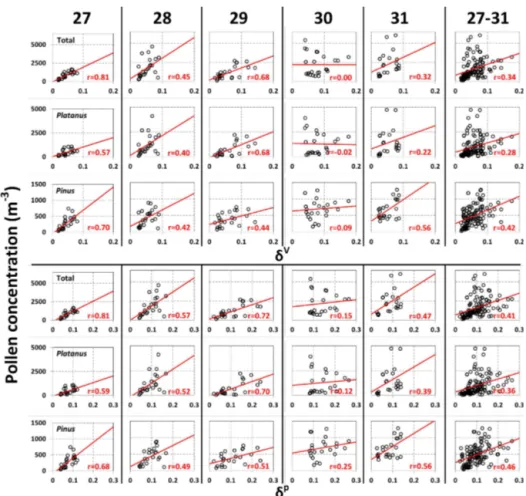
the pollen concentration. Over the whole event theδp (δV; δV−δp)rvalues are 0.41 (0.34;−0.07) for total pollen, 0.36
(0.28;−0.08) forPlatanus, and 0.46 (0.42;−0.04) forPinus.
Thus, overall theδV rvalues are between−0.08 and−0.04
smaller than theδpones. The highestδVandδprvalues are
reached forPinus(0.09< δV rvalues<0.70 and 0.25< δp r values<0.68), while the lowest r values are reached for
Platanus (0.02< δV r values<0.68 and 0.12< δp r
val-ues<0.70). One also sees that the days previously
classi-fied as days with nocturnal pollen near-surface activity (28, 30, and 31 March) have the lowestr values. This is mostly
due to the points with high concentration and low depolariza-tion ratios visible above the linear regression line, reflecting the nighttime situation of high pollen release without vertical dispersion. For the days classified as days without nocturnal pollen activity the difference betweenδVandδprvalues are
in general smaller than 0.04, so that it becomes nearly equiv-alent to useδV instead ofδp. For these days the highestδV rvalues are reached for the total pollen. Let us note that the
total pollen release and dispersion is especially well corre-lated on 27 March (δVandδprvalues are equal to 0.81). All
in all these results suggest the following.
– In all conditions, differences betweenδVandδprvalues
range between 0.08 and 0.04 andδVseems to be a proxy
better forPinusand the total pollen concentration than forPlatanusconcentration.
– Without nocturnal pollen near-surface activity,δV and δp are nearly equivalent (r values differences smaller
than 0.04) andδVseems to be an appropriate proxy for
the total pollen concentration.
Figure 6.Scatter plot of the pollen concentration (total,PlatanusandPinus) vs. the volume (δV)and the particle (δp)depolarization ratio
integrated in the pollen plume for all 5 days of the pollination event. The linear regression line is in red and the correlation coefficient,r, is
reported.
Table 3.Idem as Table 2 forPlatanus.
00:00–24:00 UT
27 28 29 30 31 27–31
PM10 −0.03 −0.10 −0.49 −0.33 −0.37 −0.19
AOD 0.14 −0.34 0.00 −0.55 −0.53 −0.22 AODpol 0.36 −0.03 0.63 −0.23 −0.32 0.01
AODpol/AOD 0.44 −0.01 0.65 −0.15 −0.15 0.07
δV 0.57 0.40 0.68 −0.02 0.06 0.26
δp 0.59 0.52 0.70 0.12 0.19 0.34
hpol 0.22 −0.44 0.36 −0.55 −0.64 −0.29
09:00–17:00 UT
27 28 29 30 31 27–31
PM10 −0.08 0.18 −0.23 −0.35 −0.03 0.04 AOD −0.23 −0.19 0.57 −0.85 −0.76 −0.33
AODpol −0.14 −0.04 0.66 −0.32 −0.67 −0.01 AODpol/AOD −0.03 −0.04 0.66 −0.11 −0.62 0.12
δV 0.18 0.74 0.70 −0.02 −0.78 0.29
δp 0.30 0.68 0.70 0.14 −0.65 0.36
hpol −0.43 −0.63 0.04 −0.72 −0.56 −0.48
5 Influence of the solar radiation on the pollen vertical transport in the atmosphere
Table 4.Idem as Table 2 forPinus.
00:00–24:00 UT
27 28 29 30 31 27–31
PM10 0.12 −0.51 −0.22 −0.39 0.32 −0.06 AOD 0.62 −0.15 −0.26 −0.75 −0.19 0.03
AODpol 0.76 0.27 0.43 −0.29 0.36 0.29
AODpol/AOD 0.80 0.27 0.55 −0.17 0.46 0.29
δV 0.70 0.42 0.44 0.09 0.44 0.42
δp 0.68 0.49 0.51 0.25 0.45 0.47
hpol 0.76 −0.19 0.63 −0.65 0.02 0.08
09:00–17:00 UT
27 28 29 30 31 27–31
PM10 −0.16 0.49 −0.21 −0.14 0.81 0.26
AOD 0.13 −0.04 −0.61 −0.86 0.27 0.02
AODpol 0.00 0.14 −0.43 −0.04 0.32 0.15
AODpol/AOD −0.03 0.17 −0.29 0.21 0.31 0.14
δV −0.45 0.45 −0.18 0.30 0.20 0.19
δp −0.79 0.38 −0.07 0.44 0.10 0.22
hpol 0.59 −0.42 −0.33 −0.54 0.29 −0.08
(also called solar irradiance) measured at ground level is the power per unit area produced by the sun in the form of elec-tromagnetic radiation measured at the Earth’s surface after atmospheric absorption and scattering.
Figure 7 shows the solar fluxes as a function of time for all 5 days of the pollination event. On 29 and 30 March clouds alter significantly the diurnal pattern of the solar radiation received at ground level. We have checked on the profiles of the MPL the presence of clouds and their altitude on the 3 clear-sky days. On 27 March, high-level clouds in the range of 9–12 km were present until 09:30 UT, while on 28 March clouds in the range of 8–10 km were present until 10:00 UT and again after 17:00 UT. On 31 March the sky was totally free of clouds with the exception of clouds forming in the ABL from 17:00 UT onwards. The possible influence of the solar radiations on the vertical transport of pollen is exam-ined with the clear-sky days of 27, 28, and 31 March. In the first row of Fig. 8 we represent all together the solar fluxes,
δV,δp, and AODpolas a function of time. Every day a diurnal
pattern is clearly visible on all curves with an increase in the morning and a decrease in the afternoon. On 27 March the temporal evolution ofδV andδpseems to follow especially
well the pattern of the solar flux. In all three cases a time delay is observed between the diurnal evolution of the solar fluxes and the depolarization ratios and of the solar fluxes and AODpol. As one could intuitively expect, the pollen ver-tical transport pattern, triggered by the turbulences caused by the heating/cooling of the ground, should follow with a given time delay (i.e., start after) that of the solar flux. The top plots of Fig. 8 clearly show that the temporal evolution of AODpol is always delayed w.r.t. the solar fluxes. In order to quantify that time delay,t, for each day, for each of the two
depolar-ization ratios and for AODpol, we have searched the value of t that maximizes the correlation coefficient defined as
0 200 400 600 800 1000
5 7 9 11 13 15 17 19
S
ol
a
r f
lu
x
(
W
m
-2)
Time of the day (UT)
27 28 29 30 31
Figure 7.Diurnal cycle for all 5 days of the pollination event of the total downward solar flux measured in the range 0.3–2.8 µm at ground level close to the lidar station.
r(t )=r (F (x), δ(x−t )) , (11)
whereF is the solar flux andδ is eitherδV,δp, or AODpol.
The optimized value oftthat maximizes the correlation
co-efficient is calledtopt. The second, third, and fourth rows of
Fig. 8 present the scatter plots of the solar flux vs.δV,δp,
and AODpol, respectively. We have represented the scatter
plots without time delay (red color,r(t=0)) and the scatter
plots with a time delay equal totopt(blue color,r(t=topt)).
TheδVrvalues without time delay are in the range of 0.49–
0.86, which already indicates a good correlation between the solar flux andδV. Ther values fort=toptare significantly
better as they range from 0.90 to 0. 95. On 27 and 31 March
topt= −1 and−2 h, respectively, which indicates that the
di-urnal pattern ofδV follows that of the solar flux delayed 1
and 2 h. On 28 Marchtopt= +1 h, which indicates that the
diurnal pattern ofδV is ahead of that of the solar flux
ap-proximately 1 h. Let us recall that 28 March is one of the days with nocturnal pollen near-surface activity and with the highest wind speeds. The maximum observed at 09:00 UT is due to a low layer of pollen (<0.5 km) with relatively high
values ofδV(see Fig. 3b). As far asδpis concerned, ther
val-ues without time delay (0.45< δpr(t=0)values<0.89) are
also significantly improved when an optimized time delay is applied (0.80< δpr(t=topt)values<0.91). The optimized
value oftforδpare the same than forδV(except on 27 March
whentopt=0 forδp). After the optimized time delay is
ap-plied,δV r values are all greater or equal to the δp r
val-ues. Differences vary between+0.03 and+0.08. These
find-ings indicate thatδVis better correlated to the solar flux than δp is. This happens probably becauseδV retrieval is much
more straightforward than δp retrieval and thus its
uncer-tainty is smaller. For AODpol, thervalues without time
de-lay (0.37<AODpol r(t=0)values<0.84) are lower than
Figure 8. (top) Diurnal evolution ofδV, δp, AODpol, and solar
fluxes on 27, 28, and 31 March between 06:00 and 18:00 UT;
(cen-ter/top) scatter plot of the solar flux vs.δV; (center/bottom) scatter
plot of the solar flux vs.δp; (bottom) scatter plot of the solar flux
vs. AODpol. In each scatter plot, straight lines are linear regression
lines; the red color corresponds tot=0; the blue color corresponds
tot=topt. The values ofr(t )are reported in each scatter plot.
negative, as foreseen from the top plot of Fig. 8 and vary between−1 and−3 h. Among the three parameters studied
(δV,δp, and AODpol), AODpolpresents the highest
correla-tion with the solar radiacorrela-tion reaching the ground. The most probable explanation of this finding is that AODpolis a
mea-sure intrinsic to pollen, whileδVandδpdepend partly on the
mixing of pollen with local aerosols.
6 Conclusion
For the first time near-surface and columnar measurements of airborne pollen have been performed continuously at a tem-poral resolution of 1 h during a 5-day pollination event in a large European city. At the peak of the event 2830 pollen and fungal spore grains were counted per cubic meter per day. Platanus andPinuspollen types represented together more than 80 % of the total concentration. Hourly concentration maxima of 4700 and 1200 m−3were found forPlatanusand
Pinus, respectively. Except on one day, the total pollen con-centration at ground level followed a clear diurnal cycle and was correlated positively with temperature (r=0.95) and
wind speed (r=0.82) but negatively with relative humidity
(r= −0.18). These results indicate a strong dependence of
pollen release upon the meteorological conditions, especially temperature and wind speed. As far as pollen AOD is con-cerned, its peaks were systematically associated with minima of relative humidity and maxima of temperature but they did not present a systematic dependence upon wind speed.
The pollen AOD showed a clear diurnal cycle with max-ima between 12:00 and 15:00 UT. The diurnal (09:00– 17:00 UT) mean of AODpolwas 0.05 over the whole event
and represented 29 % of the total AOD. However, peaks of AODpoland AODpol/AOD of, respectively, 0.12 and 78 %
were found in the hourly data. The diurnal mean volume and particle depolarization ratios in the pollen plume were 0.08 and 0.14, with hourly maxima of 0.18 and 0.33, re-spectively. The diurnal height of the pollen plume was found at 1.24 km on average with maxima varying in the range of 1.47–1.78 km.
We have investigated the possible correlations between pollen near-surface concentration and columnar properties. Between concentration and AOD (be it total or pollen AOD) the correlation was rather poor, which emphasizes that near-surface pollen release and columnar pollen dispersion are not time correlated.δVandδpwere positively correlated with the
total pollen concentration. The daily meanδVandδpr
val-ues were, respectively, 0.34 and 0.41, with maxima of 0.81 reached on the first day of the event for both parameters. When we remove the days with nocturnal pollen near-surface activity,δVandδprvalues were greater than 0.68 and their
difference smaller than 0.04.δV, and a fortioriδpappeared
to be an appropriate proxy for the total pollen concentration, especially when no pollen nocturnal activity is recorded.
The possible influence of solar radiations, which cause the atmospheric turbulences responsible for the aerosol vertical motion, on the vertical transport of pollen was examined by means ofδV,δp, AODpol, and solar fluxes measured during
the 3 clear-sky days of the pollination event. Correlation co-efficients better than 0.49 (0.45; 0.37) were obtained forδV
(δp; AODpol)vs. solar flux. In all cases we could find a time
delay between the pattern of the pollen vertical transport and the one of the solar flux that could maximize ther values.
After the optimized time delay was applied, correlation co-efficients better than 0.90 (0.80; 0.91) were obtained forδV
(δp; AODpol)vs. solar flux. This study demonstrates that, in
the absence of other depolarizing particles, the volume de-polarization ratio is an excellent tool to track airborne pollen grains. On the one hand, it is relatively well correlated with the pollen near-surface concentration which quantifies the pollen release; on the other hand, it is very well correlated with the solar fluxes on which the pollen vertical dispersion depends.
contin-uously profiles of the volume depolarization ratio are very attractive tools for modellers to validate their pollen concen-tration forecasting models and/or perform data assimilation. The question was raised for PM10concentration by Wang et al. (2013). Second, the fact that large grains of pollen (of di-ameter ranging roughly 20–70 µm) are capable of producing AOD of 0.12 raises the question of their effect in terms of radiative forcing. Otto et al. (2011) demonstrated that large mineral dust particles with a diameter of 50 µm produced a radiative forcing at the surface almost 4 times greater than the one produced by particles with a diameter of 5 µm. Large pollen grains may behave the same. Further research on that subject is definitely necessary.
Acknowledgements. Lidar data analysis was supported by the AC-TRIS (Aerosols, Clouds, and Trace Gases Research Infrastructure Network) Research Infrastructure Project funded by the European Union’s Horizon 2020 research and innovation programme under grant agreement no. 654169 and previously under grant agreement no. 262254 in the Seventh Framework Programme (FP7/2007-2013), by the Spanish Ministry of Economy and Competitiveness (projects TEC2012-34575 and TEC2015-63832-P) and of Science and Innovation (project UNPC10-4E-442) and EFRD (European Fund for Regional Development), and by the Department of Economy and Knowledge of the Catalan autonomous govern-ment (grant 2014 SGR 583). The authors also thank Xavier Lleberia and Marc Rico from the Agència de Salut Pública de
l’Ajuntament de Barcelona for providing the PM10measurements,
and the Facultad de Física of the Universitat de Barcelona for providing the meteorological measurements. Andrés Alastuey and Cristina Reche from the Instituto de Diagnóstico Ambiental y Estudios del Agua/Consejo Superior de Investigaciones Científicas
(IDÆA/CSIC) are thanked for their useful advice about the PM10
measurements.
Edited by: J. Huang
References
Alba, F., Díaz de la Guardia, C., and Comtois, P.: The effect of mete-orological parameters on diurnal patterns of airborne olive pollen concentration, Grana, 39, 200–208, 2000.
Bartková-Šcevková, J.: The influence of temperature, relative hu-midity and rainfall on the occurrence of pollen allergens (Be-tula, Poaceae, Ambrosia artemisiifolia) in the atmosphere of Bratislava (Slovakia), Int. J. Biometeorol., 48, 1–5, 2003. Behrendt, A. and Nakamura, T.: Calculation of the calibration
con-stant of polarization lidar and its dependency on atmospheric temperature, Optics Express, 10, 805–817, 2002.
Belmonte, J. and Roure, J. M.: Characteristics of the aeropollen dy-namics at several localities in Spain, Grana, 30, 361–372, 1991. Belmonte, J., Canela, M., Guàrdia, R., Guàrdia, R. A., Sbai, L.,
Vendrell, M., Cariñanos, P., Díaz de la Guardia, C., Dopazo, A., Fernández, D., Gutiérrez, M., and Trigo, M. M.: Aerobiological dynamics of the Cupressaceae pollen in Spain, 1992–98, Polen, 10, 27–38, 1999.
Boers, R., Spinhirne, J. D., and Hart, W. D.: Lidar Observations of the Fine-Scale Variability of Marine Stratocumulus Clouds, J. Appl. Meteorol., 27, 797–810, 1988.
Burch, M. and Levetin, E.: Effects of meteorological conditions on spore plumes, Int. J. Biometeorol., 46, 107–117, 2002.
Burge, H. A. and Rogers, C. A.: Outdoor allergens, Environ. Health Perspect., 108, 653–659, 2000.
Campbell, J. R., Hlavka, D. L., Welton, E. J., Flynn, C. J., Turner, D. D., Spinhirne, J. D., Scott, V. S., and Hwang, I. H.: Full-time, eye-safe cloud and aerosol lidar observation at Atmospheric Ra-diation Measurement Program sites: instruments and data pro-cessing, J. Atmos. Ocean. Tech., 19, 431–442, 2002.
Cao, X., Roy, G., and Bernier, R.: Lidar polarization discrimination of bioaerosols, Opt. Eng., 49, 76720P, doi:10.1117/12.849649, 2010.
Cecchi, L.: From pollen count to pollen potency: the molec-ular era of aerobiology, Eur. Respir. J., 42, 898–900, doi:10.1183/09031936.00096413, 2013.
Dahl, A., Galán, C., Hajkova, L., Pauling, A., Sikoparija, B., Smith, M., and Vokou, D.: The Onset, Course and Intensity of the Pollen Season, in: Allergenic Pollen. A review of the Production, Re-lease, Distribution and Health Impacts, edited by: Sofiev, M. and Bergmann, K.-Ch., 29–70, doi:10.1007/978-94-007-4881-1, Springer, 2013.
De Linares, C., Postigo, I., Belmonte, J., Canela, M., and Martínez, J.: Optimization of the measurement of outdoor airborne aller-gens using a protein microarrays platform, Aerobiologia, 30, 217–227, doi:10.1007/s10453-013-9322-2, 2014.
Denning, D. W., O’Driscoll, B. R., Hogaboam, C. M., Bowyer, P., and Niven, R.M.: The link between fungi and severe asthma: a summary of the evidence, Eur. Respir. J., 27, 615–626, 2006. Díaz de la Guardia, C., Sabariego, S., Alba, F., Ruiz, L., García
Mozo, H., Toro Gil, F. J., Valencia, R., Rodríguez Rajo, F. J., Guàrdia, A., and Cervigón, P.: Aeropalynological study of the
genusPlatanusL. in the Iberian Peninsula, Polen, 10, 89–97,
1999.
Eck, T. F., Holben, B. N., Reid, J. S., Dubovik, O., Kinne, S., Smirnov, A., O’Neill, N. T., and Slutsker, I.: The wavelength dependence of the optical depth of biomass burning, urban and desert dust aerosols, J. Geophys. Res., 104, 31333–31349, 1999. Fernald, F. G.: Analysis of atmospheric lidar observations: some
comments, Appl. Optics, 23, 652–653, 1984.
Flynn, C. J., Mendoza, A., Zheng, Y., and Mathur, S.: Novel polarization-sensitive micropulse lidar measurement technique, Opt. Express, 15, 2785–2790, 2007.
Freudenthaler, V., Esselborn, M., Wiegner, M., Heese, B., Tesche, M., Ansmann, A., Muller, D., Althausen, D., Wirth, M., Fix, A., Ehret, G., Knippertz, P., Toledano, C., Gasteiger, J., Garhammar, M., and Seefeldner, M.: Depolarizationratio profiling at several wavelengths in pure Saharan dust during SAMUM 2006, Tellus B, 61, 165–179, doi:10.1111/j.1600-0889.2008.00396.x, 2009. Gabarra, E., Belmonte, J., and Canela, M.: Aerobiological
be-haviour ofPlatanusL. pollen in Catalonia (North-East Spain),
Aerobiologia, 18, 185–193, 2002.