Optimal estimation of tropospheric H<sub>2</sub>O and δD with IASI/METOP

(1)

ACPD

11, 16107–16146, 2011

Tropospheric H₂O andδD with IASI/METOP

M. Schneider and F. Hase

Title Page

Abstract Introduction

Conclusions References

Tables Figures

◭ ◮

Back Close

Full Screen / Esc

Printer-friendly Version

Interactive Discussion

Discussion

P

a

per

|

Dis

cussion

P

a

per

|

Discussion

P

a

per

|

Discussio

n

P

a

per

|

Atmos. Chem. Phys. Discuss., 11, 16107–16146, 2011 www.atmos-chem-phys-discuss.net/11/16107/2011/ doi:10.5194/acpd-11-16107-2011

Atmospheric Chemistry and Physics Discussions

This discussion paper is/has been under review for the journal Atmospheric Chemistry and Physics (ACP). Please refer to the corresponding final paper in ACP if available.

Optimal estimation of tropospheric H

₂

O

and

δ

D with IASI/METOP

M. Schneider1,2and F. Hase1 1

Karlsruhe Institute of Technology (KIT), IMK-ASF, Karlsruhe, Germany

2

Agencia Estatal de Meteorolog´ıa (AEMET), CIAI, Santa Cruz de Tenerife, Spain

Received: 2 May 2011 – Accepted: 25 May 2011 – Published: 30 May 2011

Correspondence to: M. Schneider (matthias.schneider@kit.edu)

(2)

ACPD

11, 16107–16146, 2011

Title Page

Tables Figures

◭ ◮

Back Close

Full Screen / Esc

Discussion

P

a

per

|

Dis

cussion

P

a

per

|

Discussion

P

a

per

|

Discussio

n

P

a

per

|

Abstract

We present an optimal estimation retrieval for tropospheric H2O andδD applying

ther-mal nadir spectra measured by the instrument IASI (Infrared Atmospheric Sounding Interferometer) flown on EUMETSAT’s polar orbiter METOP. We document that the IASI spectra allow for retrieving H2O profiles between the surface and the upper

tro-5

posphere as well as middle tropospheric δD values. A theoretical error estimation suggests a precision for H₂O of better than 35 % in the lower troposphere and of better than 15 % in the middle and upper troposphere, respectively, whereby surface emis-sivity and atmospheric temperature uncertainties are the leading error sources. For the middle troposphericδD values we estimate a precision of 15–20‰, with the

mea-10

surement noise being the dominating error source. We compare our IASI products to a large number of quasi coincident radiosonde in-situ and ground-based FTS (Fourier Transform Spectrometer) remote sensing measurements and find no significant bias between the H₂O andδD data obtained by the di_fferent techniques. Furthermore, the scatter between the different data sets confirms our theoretical precision estimates.

15

1 Introduction

The continuous cycle of evaporation, vapour transport, cloud formation, and precipita-tion distributes water and energy around the globe. For reliable weather and climate predictions a thorough understanding of the atmospheric water cycle is indispensable. The complexity arises from the many di_fferent but competing processes that are

in-20

volved. For instance, upper tropospheric humidity is controlled by various processes, e.g., by diffusion, by turbulent mixing, or by detrainment of water condensates inside convective clouds. For reliable climate prediction it is important to identify the rel-ative contribution of the individual processes (upper tropospheric water vapour is a very effective greenhouse gas, Held and Soden, 2000). Water isotopologues offer

25

(3)

ACPD

11, 16107–16146, 2011

Title Page

Tables Figures

◭ ◮

Back Close

Full Screen / Esc

Discussion

P

a

per

|

Dis

cussion

P

a

per

|

Discussion

P

a

per

|

Discussio

n

P

a

per

|

different isotopologues (e.g., HD16O/H16₂ O) is a proxy for evaporation sources, condi-tions at the condensation point, and the transport process experienced by the water mass. In the following we express H16₂ O and HD16O as H₂O and HDO, respectively, and HD16O/H16₂ O asδD=1000‰ ×([HD

16_O]_/_[H16 2 O]

SMOW −1), where SMOW=3.1152×10

−4

(SMOW: Standard Mean Ocean Water, Craig, 1961).

5

The large potential of water isotopologues has been documented since several decades (e.g., Craig, 1961; Joussaume et al., 1984; Worden et al., 2007; Yoshimura et al., 2008). However, even today research in this field is still limited by the lack of consistent, long-term, high-quality, and area-wide observational data. The reason is that water isotopologue ratio measurements are very difficult. Compared to the

over-10

all variability of tropospheric water concentrations the variability in the isotopologue ratios is rather small and detecting such low variations requires highly-precise mea-surement techniques. In the past such stringent precision requirements have nearly exclusively been achieved by in-situ techniques and most tropospheric water isotopo-logue data have been collected during a few dedicated in-situ measurement campaigns

15

(e.g. Ehhalt, 1974; Zahn, 2001; Webster and Heymsfield, 2003).

Recently, there has been large progress in observing tropospheric water isotopo-logues by remote sensing techniques. Schneider et al. (2006b, 2010b) document the possibility of the global network of FTS (Fourier Transform Spectrometer) systems for a ground-based remote sensing of tropospheric H2O and δD profiles. Worden et

20

al. (2006) and Frankenberg et al. (2009) show that the sensors TES (Tropospheric Emission Spectrometer) aboard AURA and SCIAMACHY (Scanning Imaging Absorp-tion Spectrometer for Atmospheric Chartography) aboard ENVISAT allow for a space-based remote sensing of tropospheric H₂O and δD. The remote sensing techniques can provide continuous data sets and – if performed from space – they offer the

possi-25

bility for quasi global scale observations.

(4)

ACPD

11, 16107–16146, 2011

Title Page

Tables Figures

◭ ◮

Back Close

Full Screen / Esc

Discussion

P

a

per

|

Dis

cussion

P

a

per

|

Discussion

P

a

per

|

Discussio

n

P

a

per

|

H16₂ O and HD16O has been demonstrated by Herbin et al. (2009). Although IASI’s spectral resolution is lower than TES’s resolution it is very likely that IASI is able to de-tect troposphericδD. IASI is very interesting for water cycle research, since it is flown aboard the operational meteorological satellite METOP and combines global coverage with high horizontal and temporal resolution: despite its small pixel size of 12 km

diam-5

eter it covers almost the whole globe twice per day. Furthermore, IASI measurements will be guaranteed between 2006 and 2020 on a series of three METOP satellites.

In this paper we document that IASI can indeed detect troposphericδD in addition to tropospheric H₂O. In Sect. 2 we present the applied retrieval method. Section 3 shows a theoretical estimate of the quality of our IASI H2O and δD products and in

10

Sect. 4 we empirically validate them. Therefore, we compare the IASI data to a large number of in-situ radiosonde measurements of H₂O as well as to ground-based FTS remote sensing measurements of H2O andδD, which are made in coincidence to IASI

overpasses.

2 The retrieval

15

2.1 The PROFFIT-nadir retrieval code

The thermal nadir retrieval code PROFFIT-nadir has been very recently developed as an extension to PROFFIT (Hase et al., 2004), which has been applied since many years by the ground-based FTS community for evaluating high resolution solar absorption spectra.

20

The code simulates the spectra and the Jacobians by the line-by-line radiative trans-fer model PRFFWD (Schneider and Hase, 2009a). It includes a ray tracing module (Hase and H ¨opfner, 1999) in order to precisely simulate how the radiation passes through the atmosphere. The vertical structure of the atmosphere is discretised and the amount of the absorberx at altitude levelz can be described in form of a vectorx(z).

25

(5)

ACPD

11, 16107–16146, 2011

Title Page

Tables Figures

◭ ◮

Back Close

Full Screen / Esc

Discussion

P

a

per

|

Dis

cussion

P

a

per

|

Discussion

P

a

per

|

Discussio

n

P

a

per

|

a vectory containing the radiances at the different spectral bins. PRFFWD accounts for the forward relation (F), that connects the spectrum (y) to the vertical distribution of the absorbers (x) and to parameters (p) describing the state of the surface-atmosphere system as well as instrumental characteristics:

y₌F(x,p) (1)

5

The retrieval consists in adjusting the amount of the absorbers so that simulated and measured spectra agree. This is an under-determined problem, i.e., there are many different atmospheric states (x) that produce almost identical spectra (y). Con-sequently the problem requires some kind of regularisation. PROFFIT introduces the regularisation by means of a cost function:

10

[y₋F(x,p)]TS_ǫ−1

[y₋F(x,p)]+[x₋x_a]TS_a−1

[x₋x_a] (2)

Here the first term is a measure for the difference between the measured spectrum (y) and the spectrum simulated for a given atmospheric state (x), whereby the actual measurement noise level is considered (S_ǫis the noise covariance). The second term is the regularisation term. It constrains the atmospheric solution state (x) towards an

15

a priori state (xa), whereby the kind and the strength of the constraint are defined by

the matrixS_a. The constrained solution is reached at the minimum of the cost function Eq. (2).

Since the equations involved in atmospheric radiative transfer are non-linear, Eq. (2) is minimised iteratively by a Gauss-Newton method. The solution for the (i+1)th

iter-20

ation is:

xi+1=xa+S_aK_i

T

(K_iS_aK_iT+S_ǫ)−1

[y₋F(xi)+K_i(xi₋xa)] (3)

WherebyKis the Jacobian matrix which samples the derivatives ∂y/∂x (changes in

the spectral fluxesy for changes in the vertical distribution of the absorberx).

These regularisation and iteration methods are standard in the field of remote

sens-25

(6)

ACPD

11, 16107–16146, 2011

Title Page

Tables Figures

◭ ◮

Back Close

Full Screen / Esc

Discussion

P

a

per

|

Dis

cussion

P

a

per

|

Discussion

P

a

per

|

Discussio

n

P

a

per

|

In addition to these standard methods PROFFIT allows for a logarithmic scale re-trieval. Therefore, the atmospheric state vector, the a priori state and the a priori ma-trix, and the Jacobians have to be transferred on a logarithmic scale. This option is often called a positivity constraint since it assures positive solutions. It has proven to be very beneficial for tropospheric water vapour retrievals. The reason is that

tro-5

pospheric water vapour concentrations are rather log-normally and not normally dis-tributed, therefore the regularisation term of Eq. (2) is only adequately working on a log-scale (Schneider et al., 2006a).

The log-scale retrieval is also required for constraining ratios of absorbing species. Since ln[HDO]_[H

2O] =ln[HDO]−ln[H2O] we can easily introduce an HDO/H2O constraint in 10

the regularisation term of Eq. (2) (we only have to fill in the respective elements of the matrixS_a, Schneider et al., 2006b).

Furthermore, PRFFWD supports different spectroscopic line shape models, which is particularly important when retrieving water vapour profiles from very high resolution spectra (Schneider et al., 2011).

15

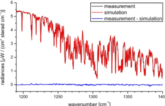
2.2 The IASI H₂O andδD retrieval

IASI records the thermal infrared emission of the Earth-atmosphere system between 645 and 2760 cm−1with an apodized spectral resolution of 0.5 cm−1. Figure 1 shows an IASI measurement, a simulation of this measurement, and the di_fference of both of the spectral window that we apply for our retrieval. The selected spectral window

20

covers the region between 1190 and 1400 cm−1. In this region there are strong lines of di_fferent water vapour isotopologues. Beside the main isotopologue H16₂ O, the sec-ondary isotopologues H18₂ O, H17₂ O, and HD16O are important. In addition, there are significant spectroscopic features of CH₄ and N₂O and minor features of HNO₃, CO₂, and O3(a nice overview of the individual spectroscopic features in the selected

spec-25

(7)

ACPD

11, 16107–16146, 2011

Title Page

Tables Figures

◭ ◮

Back Close

Full Screen / Esc

Discussion

P

a

per

|

Dis

cussion

P

a

per

|

Discussion

P

a

per

|

Discussio

n

P

a

per

|

(Rothman et al., 2009).

Except for O₃, whose weak signatures are only included in the forward calculation by assuming a climatological profile, all these species are simultaneously retrieved: while for CO2 we scale a climatological profile, for CH4, N2O, and HNO3 we apply a more

relaxed ad hoc regularisation and allow for changes in the shape of a climatological

5

profile. All these interfering species are retrieved on a linear scale.

The targeted water isotopologues are retrieved on a log-scale and regularised in an optimal estimation manner, in the sense that the a priori matrixS_aof Eq. (2) is deduced from the tropospheric water vapour covariances observed by radiosonde measure-ments: up to 12.5 km we use an a priori 1σ variability of 1.0 (on log scale!), between

10

12.5 and 25 km it decreases linearly to 0.25, and for higher altitudes it remains constant at 0.25. The correlation lengths between the different altitude levels increase linearly from 2.5 km in the lower troposphere to 10 km in the stratosphere. On the log-scale we can use the sameS_a for the di_fferent water isotopologues. We treat the H16₂ O, H18₂ O, and H17₂ O isotopologues as a group and distinguish it from the HD16O isotopologue.

15

This is justified since the fractionations between the oxygen isotopologues are typically one order of magnitude smaller than their fractionation with respect to the deuterium isotopologue. The applied H2O log-scale a priori profile (xaof Eq. 2) linearly decreases

from the lower troposphere up to 15 km, whereby the slope of the decrease is deduced from radiosonde data sets. In the stratosphere we use a H2O climatology obtained

20

from MIPAS observations (J. J. Remedios, private communication, 2007).

The HDO a priori profile is calculated from the H₂O profile using the (ln[HDO]−

ln[H₂O]) climatology of Ehhalt (1974). From the Ehhalt (1974) measurements we also deduce the (ln[HDO]−ln[H2O]) elements of theSamatrix: an 1σ−(ln[HDO]−ln[H2O])

variability of 80‰ and a correlation length between the different altitude levels which is

25

identical to the one for ln[H₂O] (linear increase from 2.5 km in the lower troposphere to 10 km in the stratosphere).

(8)

ACPD

11, 16107–16146, 2011

Title Page

Tables Figures

◭ ◮

Back Close

Full Screen / Esc

Discussion

P

a

per

|

Dis

cussion

P

a

per

|

Discussion

P

a

per

|

Discussio

n

P

a

per

|

IASI level 2 temperatures. In the case of the atmospheric temperature retrieval the constraint is rather strong (S_adiagonal variances of 0.252K2). In this study we select observations over the ocean and thus use a constant surface emissivity of 1.0.

Concerning cloud detection we rely on EUMETSAT’s IASI level 2 cloud product. We only evaluate pixel that are measured for cloud free conditions, whereby we define as

5

cloud free if EUMETSAT’s level 2 fractional cloud cover parameter is below 15 %. For more details about EUMETSAT’s level 2 cloud products please refer to the EUMETSAT IASI level 2 product guide (2011).

In this study we only work with IASI morning overpasses.

3 Product characterisation

10

3.1 Vertical resolution and sensitivity

An important addendum of the retrieved solution vector is the averaging kernel matrix

A. It samples the derivatives ∂x/∂xˆ (changes in the retrieved concentration ˆx for changes in the actual atmospheric concentration x describing the smoothing of the real atmospheric state by the remote sensing measurement process:

15

(xˆ₋xa)=A(x₋xa) (4)

In addition, the trace ofAquantifies the amount of information introduced by the mea-surement. It can be interpreted in terms of degrees of freedom (DOF) of the measure-ment.

Concerning differences in ln[H2O] and (ln[HDO]−ln[H2O]) we can write:

20

∆(ln[H2O])≈

∆[H₂O]

(9)

ACPD

11, 16107–16146, 2011

Title Page

Tables Figures

◭ ◮

Back Close

Full Screen / Esc

Discussion

P

a

per

|

Dis

cussion

P

a

per

|

Discussion

P

a

per

|

Discussio

n

P

a

per

|

and

∆(ln[HDO]−ln[H2O])≈

∆[HDO]_[H

2O]

[HDO] [H₂O]

=

∆[HDO]_[H

2O]

+[HDO]_[H

2O]

[HDO] [H₂O]

−1 (6)

Therefore, in the following we will use differences in ln[H2O] interchangeably with

rela-tive differences in [H2O] and differences in (ln[HDO]−ln[H2O]) with differences in δD.

Figure 2 shows the averaging kernels for a typical IASI H₂O retrieval over the ocean

5

(surface temperature 290 K) and for cloud free conditions. The left panel depicts the column kernels. They describe the response of the retrieved state vector on a 1.0 disturbance of the real state vector. We can observe that the maxima of these response functions generally peak at the altitude of the disturbances: the black line describes the response for an 1.0 disturbance at 0.5 km and it peaks close to 0.5 km, the red

10

line represents the response on a disturbance at 3 km and it peaks close to 3 km, etc. The FWHM (full width at half maximum) of these kernels can be interpreted as the vertical resolution of the remote sensing measurement. We find FWHMs of about 2.5, 4.5, and 9 km for the lower, middle, and upper troposphere, respectively. The sum of the column kernels (depicted as thick black line) indicates the overall sensitivity of

15

the retrieved state with respect to the real state. IASI is well sensitive with respect to atmospheric H₂O from the surface up to 13 km (sensitivity better than 75 %). For the cloud free H2O retrievals we find a typical DOF value of 3.4.

The right panel of Fig. 2 shows the rows of the averaging kernel matrix. They indicate the altitude regions that mainly contribute to the retrieved state. We see that the state

20

retrieved at different altitudes, e.g., 0.5, 3, 6.5, and 10 km, reflects well the real state at these altitudes.

Figure 3 depicts the same as Fig. 2 but for δD. In contrast to H₂O our IASI δD retrieval can not resolve profiles of δD. Only in the lower troposphere the sensitivity (sum of column kernels) is close to 75 %. Above 3 km it starts to decrease steadily.

25

(10)

ACPD

11, 16107–16146, 2011

Title Page

Tables Figures

◭ ◮

Back Close

Full Screen / Esc

Discussion

P

a

per

|

Dis

cussion

P

a

per

|

Discussion

P

a

per

|

Discussio

n

P

a

per

|

δD state between 2 and 5.5 km. Over the ocean and under cloud free conditions we can only detectδD variation in this altitude range. Our IASI δD sensitivity estimate is similar to the one obtained by Worden et al. (2006) for TES.

3.2 Propagation of uncertainty sources

We consider three groups of uncertainty sources: (1) uncertainty in the thermal

radia-5

tion emitted by the Earth-atmosphere system, (2) uncertainty in the spectroscopic line parameter of the water isotopologues, (3) uncertainty due to spectroscopic features of interfering species, and (4) measurement noise. The propagation of these uncertain-ties can be calculated by (e.g., Rodgers, 2000):

δx₌GK_pǫp (7)

10

WherebyGis the gain matrix, which samples the derivatives ∂x/∂yˆ (changes in the retrieved state ˆx for changes at the spectral bin y), K_p is the parameter Jacobian, which samples the derivatives∂y/∂p(changes at the spectral biny for changes in the parameterp), andǫpis a vector describing the uncertainty of parameterp.

3.2.1 Thermal radiation

15

IASI measures the thermal radiation emitted by the Earth-atmosphere system. The intensity and broadband characteristic of this radiation depends on the emissivity and temperature of the Earth’s surface and on the atmospheric vertical temperature profile. Thus the emissivity and temperatures importantly affect the interpretation of an IASI measurement. For the surface emissivity we assume an uncertainty of+5 % (we

cal-20

(11)

ACPD

11, 16107–16146, 2011

Title Page

Tables Figures

◭ ◮

Back Close

Full Screen / Esc

Discussion

P

a

per

|

Dis

cussion

P

a

per

|

Discussion

P

a

per

|

Discussio

n

P

a

per

|

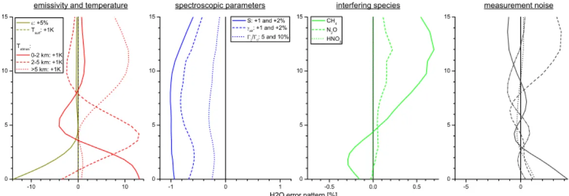
The leftmost panel of Fig. 4 documents how these uncertainties propagate into the retrieved H₂O profiles. An erroneously too large emissivity will lead to a significant underestimation of boundary layer H2O. Uncertainties in the surface temperature are

effectively identified by the surface temperature retrieval and do not significantly affect the retrieved H₂O profiles. This is in contrast to uncertainties in atmospheric

tem-5

peratures which strongly interfere with the retrieved H2O: if the assumed atmospheric

temperature is by 1 K too large the retrieval overestimates the H2O amounts by up to

15 %.

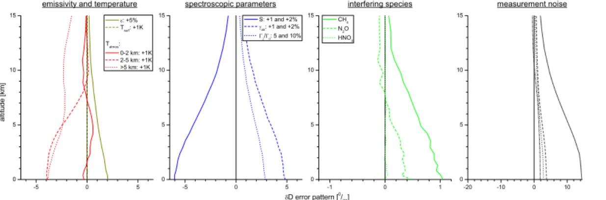
Figure 5 shows the respective δD error patterns. It documents that for δD at-mospheric temperature errors above 2 km are dominating this group of uncertainty

10

sources.

3.2.2 Spectroscopic parameters

The line-by-line modelling relies on the parameters collected in spectroscopic databases like HITRAN (Rothman et al., 2009). For our estimation we consider the line parameter uncertainty as collected in Table 2: the line strength (S), the air

pres-15

sure broadening coefficient (γair), and the applied line shape model (strength of

speed-dependence: Γ2/Γ0, D’Eu et al., 2002). In Schneider et al. (2011) it has been

doc-umented that the application of di_fferent line shape models strongly a_ffect the H₂O profiles estimated from very high resolution spectra.

We assume different errors for the H2O and HDO isotopologues in order to

esti-20

mate how an inconsistency between the H₂O and HDO line parameters a_ffects theδD retrievals.

The line strength parameter dominates the spectroscopic parameter uncertainty (see second panel form the left of Fig. 4). For thermal nadir sounding with a spectral res-olution of 0.5 cm−1 the line shape is of secondary importance In ground-based solar

25

(12)

ACPD

11, 16107–16146, 2011

Title Page

Tables Figures

◭ ◮

Back Close

Full Screen / Esc

Discussion

P

a

per

|

Dis

cussion

P

a

per

|

Discussion

P

a

per

|

Discussio

n

P

a

per

|

ForδD the spectroscopic line parameter uncertainties are of similar importance than the emissivity and temperature uncertainties (compare first and second panel from the left of Fig. 5). This is in contrast to H2O, where the errors due spectroscopic

line parameter uncertainties are much smaller than the errors due to emissivity and temperature uncertainties. The reason for the relatively low importance of emissivity

5

and temperature uncertainties in the case ofδD is that these uncertainties propagate similarly into H2O and HDO and widely cancel out when calculating the ratio, whereas

inconsistency in the H₂O and HDO line parameters do not cancel out.

3.2.3 Interfering species

In the analysed spectral window there are also important spectral signatures of CH4,

10

N2O, and HNO3. These signatures might interfere with the signatures of the water

iso-topologues and thus a_ffect the retrieved H₂O andδD. In order to assess the importance of this interference we increase the line strength (S) and the pressure broadening pa-rameters (γair) of these species by 2 % and observe the impact on the H2O and δD

retrievals. ChangingS andγairhas a similar effect on the spectra as changing the total

15

column amount and the vertical distribution of the absorber.

The third panel from the left of Figs. 4 and 5 document that CH4is the most important

interfering species. The interfering errors of N₂O are rather small and the ones of

HNO3 can be completely neglected. Concerning H2O the upper tropospheric CH4

interfering errors are almost as important as respective errors due to uncertainties in

20

the spectroscopic parameters of H₂O.

3.2.4 Measurement noise

Naturally noise in the measured spectra will lead to random errors in the retrieved prod-ucts. When calculating the propagation of the measurement noise we can substitute

K_pǫp in Eq. (7) by the vector ǫy representing the noise at each spectral bin. For our 25

(13)

ACPD

11, 16107–16146, 2011

Title Page

Tables Figures

◭ ◮

Back Close

Full Screen / Esc

Discussion

P

a

per

|

Dis

cussion

P

a

per

|

Discussion

P

a

per

|

Discussio

n

P

a

per

|

which is an IASI radiometric noise value that has been established from a set of repre-sentative spectra (Clerbaux et al., 2009, Fig. 2). The four leading error noise patterns are depicted in the rightmost panel of Figs. 4 and 5.

For H₂O we observe largest errors in the lower and upper troposphere, whereby the sign of these errors is partly anti-correlated, i.e., large positive errors in the lower

5

troposphere often come along with negative errors in the upper troposphere (see error pattern represented by the solid grey line). In the middle troposphere measurement noise seems to be less important than in the lower and upper troposphere.

ForδD the measurement noise error patterns have no significant vertical structure, i.e., they are of the same sign at all altitude levels.

10

3.2.5 Random error budget

The uncertainties of surface temperature and emissivity, atmospheric temperatures, concentration profiles of interfering species, and the measurement noise contribute to the overall random error budget. The random error of each group can be calculated as the root-square-sum of the individual contributions, e.g., the atmospheric temperature

15

random error is the root-square-sum of the atmospheric temperature error patterns as depicted in the leftmost panels of Figs. 4 and 5: qT₀2

−2km+T

2

2₋5km+T 2

>5km. In addition

GandK_p of Eq. (7) slightly depend on the surface conditions, atmospheric conditions, and on IASI’s observation geometry, i.e., the patterns of Figs. 4 and 5 slightly vary from observation to observation. This additional random error contribution is considered in

20

the budgets presented in Fig. 6 and it is the reason why even a systematic uncertainty source, like the uncertainties in the spectroscopic line parameters of H2O and HDO

produce a random error component (see blue curves in Fig. 6).

Concerning H2O the total random error (thick black line) is dominated by the

un-certainties in the atmospheric temperature (red line). Furthermore, in the lower

tro-25

(14)

ACPD

11, 16107–16146, 2011

Title Page

Tables Figures

◭ ◮

Back Close

Full Screen / Esc

Discussion

P

a

per

|

Dis

cussion

P

a

per

|

Discussion

P

a

per

|

Discussio

n

P

a

per

|

We estimate a IASIδD precision of about 18‰. It is clearly controlled by the mea-surement noise, which is the leading random error (see dark grey line in the right panel of Fig. 6). The reason is that most other errors propagate similarly into H2O and HDO

and thus cancel out in the H₂O/HDO ratio.

These estimations document, that IASI’s low noise level is decisive for its δD

re-5

mote sensing capability: troposphericδD variations are typically 80‰. If IASI’s noise level was four times higher the total δD random error would be close to 80‰ and a single IASI measurement pixel would hardly reach the precision level required for the observation of troposphericδD.

4 Product validation

10

The scientific value of this new IASI observational data strongly depends on the doc-umentation of its quality. While there are H2O data available from various techniques

that can serve as a validation reference (e.g., meteorological radiosondes) there is cur-rently only one technique that can measureδD at different tropospheric altitudes and on a regular basis: the ground-based FTS technique (Schneider et al., 2010b). In this

15

section we show a comparison of our IASI products to data from Vaisala radiosondes and from a ground-based FTS system.

4.1 The validation site

Figure 7 shows a map of the western part of the Canary archipelago situated in the northern subtropical Atlantic Ocean about 300 km west of the African west

20

coast at about 28◦N. The center of the map shows Tenerife, the main Island of the Western Canary province. It hosts the Iza ˜na Atmospheric Research Centre (IARC, www.aemet.izana.org, indicated as red dot in the centre of Tenerife). IARC is run by the Meteorological State Agency of Spain (AEMET) and has been contributing since many years with high-quality atmospheric observations to a variety of international

(15)

ACPD

11, 16107–16146, 2011

Title Page

Tables Figures

◭ ◮

Back Close

Full Screen / Esc

Discussion

P

a

per

|

Dis

cussion

P

a

per

|

Discussion

P

a

per

|

Discussio

n

P

a

per

|

atmospheric monitoring networks. Since 1999 high resolution infrared solar absorption spectra have been recorded by a ground-based FTS system. The high quality of the tropospheric H2O andδD measured at Iza ˜na has been demonstrated in several studies

(e.g., Schneider et al., 2010a,b). About 20 km east of the observatory on the coastline there is a launch pad for meteorological radiosondes (indicated as yellow dot in Fig. 7).

5

There Vaisala RS92 radiosondes are launched twice per day at 00:00 and 12:00 UT. The red and yellow arrows denote the airmass that is typically analysed during the IASI morning overpasses by the FTS system and the radiosonde, respectively. The cyan circles mark IASI cloud free pixels (12 km diameter) that fall within the selected valida-tion box between 27.3 and 28.3◦N and 17.0 and 16.0◦W (indicated by the black dotted

10

lines) and that have been measured between March and June 2009 within 60 min of an RS92 or FTS observation. Table 3 shows the number of measurements that have been used for this validation exercise.

4.2 Comparison to meteorological radiosondes Vaisala RS92

We correct the radiosonde humidity data by the formulas given in V ¨omel et al. (2007).

15

Furthermore, we adjust the vertically highly-resolved Vaisala RS92 profile (x_RS92) to the limited vertical resolution of the IASI profiles. Therefore, we convolvex_RS92 with the averaging kernels. According to Eq. (4) it is:

ˆ

x_RS92₌A(x_RS92₋x_a)+x_a (8)

The result is an RS92 profile (xˆ_RS92) with the same vertical resolution and sensitivity

20

as the IASI profile.

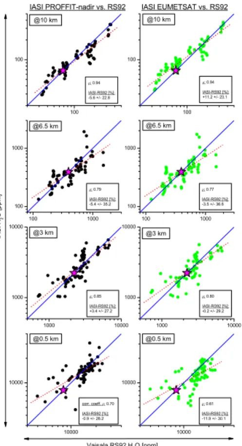
The left panels of Fig. 8 show correlations between the H2O concentrations obtained

by the RS92 and IASI at different altitudes. With the exception of the boundary layer, the correlation coefficients are about 0.8 or higher. In particularly nice is the correlation in the upper troposphere at 10 km (correlation coefficient of 0.94).

25

(16)

ACPD

11, 16107–16146, 2011

Title Page

Tables Figures

◭ ◮

Back Close

Full Screen / Esc

Discussion

P

a

per

|

Dis

cussion

P

a

per

|

Discussion

P

a

per

|

Discussio

n

P

a

per

|

We observe no significant bias. The mean difference lies almost within±5 %

through-out the troposphere. Figure 9 shows a profile of this IASI-RS92 di_fferences (black line and error bars for mean differences and standard deviation of the differences, respec-tively). It nicely documents the good overall agreement between our IASI H2O products

and the Viasala RS92.

5

4.3 Comparison between PROFFIT-nadir and EUMETSAT level 2 products

In addition we compared to EUMETSAT level 2 H2O products (in the following called

EUM H2O). EUMETSAT documents a vertical resolution of its level 2 H2O profiles of

about 1–2 km (e.g., EUMETSAT IASI level 2 product guide, 2011, Figs. 4–6). This is by far better than the resolution that we obtain from our calculations. Therefore, we treat

10

the EUM data with our averaging kernels. The so-smoothed EUM profiles should have the same characteristics than our IASI PROFFIT-nadir profiles.

In order to assess the quality of the EUM data we correlate and compare them to the RS92 data. The results of this assessment are shown in the right panels of Fig. 8 and depicted as green curve in Fig. 9. The correlation coe_fficients are very similar to the

15

coefficients we obtained for the correlation between PROFFIT-nadir IASI products and RS92. In both cases we observe that the correlation coefficients tend to increase from the lower to the upper troposphere, which is in agreement with lower and middle tropo-spheric humidity fields being more inhomogeneous than upper tropotropo-spheric humidity fields: in the lower and middle troposphere our comparison is much more affected by a

20

mismatch in the airmass analysed by IASI, on the one hand, and by the RS92, on the other hand, than in the upper troposphere.

In the boundary layer the correlation between EUM and RS92 is slightly poorer than the correlation between the IASI PROFFIT-nadir product and the RS92. Furthermore, concerning systematic differences we observe that above 10 km the EUM

concentra-25

tions overestimate the RS92 concentrations (see green curve in Fig. 9).

(17)

ACPD

11, 16107–16146, 2011

Title Page

Tables Figures

◭ ◮

Back Close

Full Screen / Esc

Discussion

P

a

per

|

Dis

cussion

P

a

per

|

Discussion

P

a

per

|

Discussio

n

P

a

per

|

it documents the nice consistency between different IASI H₂O retrievals: above the boundary layer we obtain correlation coefficients of larger than 0.98. However, it has to be noted that our retrieval uses the EUMETSAT temperature profiles as the a priori temperature, so the EUM and PROFFIT-nadir H₂O products are not fully independent. Concerning the upper troposphere we can clearly identify a systematic wet bias of

5

EUM with respect to PROFFIT-nadir. At 13 km this bias reaches 25 % (see Fig. 11). In the boundary layer the correlation between the two IASI retrievals is rather poor. This suggests that the relatively poor agreement between the IASI EUM and PROFFIT-nadir H2O, on the one hand, and the RS92 H2O, on the other hand – as documented

in the bottom layers of Fig. 8 – is not exclusively due to the aforementioned increased

10

inhomogeneities at low altitudes. Instead, very close to the surface the IASI H₂O re-trievals seem to be significantly less precise than at higher altitudes. This is exactly what is predicted by the error estimation (see Fig. 6), which indicates that close to the surface the quality of the IASI H₂O data strongly depends on the uncertainties of surface emissivity and lower tropospheric temperatures.

15

4.4 Comparison to ground-based FTS

Comparing ground-based FTS data to IASI data means comparing two different

re-mote sensing systems with di_fferent sensitivities. Some examples of typical H₂O and

δD kernels obtained when analysing ground-based FTS spectra are shown in Fig. 3 of Schneider et al. (2010b). In particularly forδD the FTS and IASI kernels differ

signifi-20

cantly. Furthermore, when taking the FTS data from Iza ˜na we have to consider that the instrument measures solar absorption spectra and that it is situated at 2370 m a.s.l.: it is not sensitive to the atmosphere below 2370 m a.s.l.

In order to support this IASI ground-based FTS comparison study we performed the FTS retrievals on the same altitude grid as the IASI retrievals and in addition applied

25

(18)

ACPD

11, 16107–16146, 2011

Title Page

Tables Figures

◭ ◮

Back Close

Full Screen / Esc

Discussion

P

a

per

|

Dis

cussion

P

a

per

|

Discussion

P

a

per

|

Discussio

n

P

a

per

|

averaging kernels of the two remote sensing systems can be estimated by:

S_δx₌(A_IASI−AFTS)Sa(AIASI−AFTS)T (9)

HereS_δxis a matrix containing the covariances of the inherent scatter when comparing IASI with FTS,S_ais the known a priori covariance of H2O andδD, andAIASIandAFTS

are the IASI and FTS averaging kernels, respectively.

5

The ground-based FTS systems allow for an optimal estimation of tropospheric H2O andδD in two different spectral regions (1090–1330 cm−

1

and 2650–3025 cm−1, Schneider et al., 2010c). Figure 12 shows the square root values of the diagonal elements of S_δx: left panel for H2O and right panel for δD. The black solid line for

the FTS retrievals at 1090–1330 cm−1and the red dotted line for the FTS retrieval at

10

2650–3025 cm−1_{. The blue dotted line indicates the altitude of the ground-based FTS}

system.

Concerning H2O both remote sensing data are well comparable between 3 and 9 km.

At higher altitudes IASI is more sensitive than the FTS system and consequently both data set are less comparable. Close to the altitude of Iza ˜na the completely missing

15

sensitivity of the FTS for lower tropospheric H2O makes the two data set not

compara-ble.

For δD the remote sensing data are best comparable at 4–5 km altitude. This is an altitude where IASI is still sufficiently sensitive and where the impact of the FTS system’s missing lower tropospheric sensitivity is less important than at lower altitudes.

20

Figure 13 shows correlations between the IASI and the FTS H2O concentrations for

the altitudes marked in the left panel of Fig. 12 by the black thick dots and the red triangles: 3 km, 5 km, and 9 km. For both FTS retrievals the correlation coefficients are situated between 0.84 and 0.89. This nice agreement confirms the results of the comparison with the RS92 H2O data.

25

(19)

ACPD

11, 16107–16146, 2011

Title Page

Tables Figures

◭ ◮

Back Close

Full Screen / Esc

Discussion

P

a

per

|

Dis

cussion

P

a

per

|

Discussion

P

a

per

|

Discussio

n

P

a

per

|

For both cases the statistics of the IASI-FTSδD differences reveals no significant dif-ference. The standard deviation of this difference is about 50 and 40‰. Figure 14 reveals that the regression line slope is significantly less steep than unity. This is in agreement with IASI’s δD sensitivity being less than 100 % (see Fig. 3) and with the FTS’sδD sensitivity being close to 100 % at this altitude (e.g., Schneider et al., 2010c).

5

For both comparisons we find similar correlation coefficients of about 0.85. More than 70 % of the variance of both FTS δD retrievals is also observed by IASI (ρ2=

0.852=0.723 is the portion of the variance that is equally captured by two compared data sets). Only for the remaining 30 % variance FTS and IASI disagree, whereby this 30 % is not only due to errors in theδD data. It is also partly due to a mismatch

10

of the airmass remotely-sensed by the FTS and IASI, respectively, and due to the aforementioned incomparability of the two remote sensing systems.

Systematic errors in the IASI and FTS data are theoretically dominated by uncer-tainties in di_fferent spectroscopic line parameters. In case of the FTS data a very high accuracy of the parameters that describe the spectroscopic line shape (e.g.,γair and

15

Γ2/Γ0, Schneider et al., 2010c) is important. This is in contrast to the IASI data, where

uncertainties in the line strength are dominating (see second panels of Figs. 4 and 5). Obviously there is no reason to expect a correlation of IASI’s and FTS’s system-atic errors, so the absence of significant systemsystem-atic differences between IASI’s and the FTS’s H₂O andδD as observed in this study is indeed remarkable. It documents that

20

– in the meanwhile and after the careful developments during the last years – both the ground-based solar absorption FTS and the space-based thermal nadir remote sensing techniques have reached a major status of maturity.

5 Conclusions

We show that IASI thermal nadir spectra allow for an optimal estimation of middle

tro-25

(20)

ACPD

11, 16107–16146, 2011

Title Page

Tables Figures

◭ ◮

Back Close

Full Screen / Esc

Discussion

P

a

per

|

Dis

cussion

P

a

per

|

Discussion

P

a

per

|

Discussio

n

P

a

per

|

(dominated by atmospheric temperature uncertainties) of 35 % in the boundary layer and 15 % in the middle and upper troposphere. We estimate a sensitivity of IASI with respect to the realδD state of about 70 %. ForδD errors due to temperature uncer-tainties widely cancel out (since errors cancel out when calculating the HDO/H2O ratio)

and the precision is controlled by measurement noise. It is about 18‰.

5

Our IASI H2O product well agrees with meteorological radiosondes and with the

EUMETSAT level 2 product. The increased discrepancies close to the surface are in agreement with the theoretical estimations.

The comparison of the IASI H2O and δD data to data obtained by a ground-based

FTS system show a remarkable consistency. Both IASI and the FTS system observe

10

very similar lower to upper tropospheric H₂O and middle troposphericδD values. There are no significant systematic differences between the IASI and the FTS data. These results allow for combining both remote sensing techniques. Such combination would take benefit from both the long-term characteristics of the historic ground-based FTS observations (FTS activities date back to the 1990s at about 15 globally distributed

15

stations) and the wide geographical coverage of the space-based IASI observations. We plan to perform this task in the near future in the framework of the project MU-SICA (MUlti-platform remote Sensing of Isotopologues for investigating the Cycle of Atmospheric water, www.imk-asf.kit.edu/english/musica).

Acknowledgements. We thank Maxim Eremenko for his support with EUMETSAT’s IASI data 20

dissemination and formats. This study has been conducted in the framework of the project MUSICA which is funded by the European Research Council under the European Community’s Seventh Framework Programme (FP7/2007-2013)/ERC Grant agreement number 256961.

(21)

ACPD

11, 16107–16146, 2011

Title Page

Tables Figures

◭ ◮

Back Close

Full Screen / Esc

Discussion

P

a

per

|

Dis

cussion

P

a

per

|

Discussion

P

a

per

|

Discussio

n

P

a

per

|

References

Clerbaux, C., Boynard, A., Clarisse, L., George, M., Hadji-Lazaro, J., Herbin, H., Hurtmans, D., Pommier, M., Razavi, A., Turquety, S., Wespes, C., and Coheur, P.-F.: Monitoring of atmo-spheric composition using the thermal infrared IASI/MetOp sounder, Atmos. Chem. Phys., 9, 6041–6054, doi:10.5194/acp-9-6041-2009, 2009. 16109, 16119

5

Craig, H.: Standard for Reporting Concentrations of Deuterium and Oxygen-18 in Natural Wa-ters, Science, 133, 1833–1834, doi:10.1126/science.133.3467.1833, 1961. 16109

D’Eu, J.-F., Lemoine, B., and Rohart, F.: Infrared HCN Lineshapes as a Test of Galatry and Speed-dependent Voigt Profiles, J. Molec. Spectrosc., 212, 96–110, 2002. 16117

Ehhalt, D. H.: Vertical profiles of HTO, HDO, and H₂O in the Troposphere, Rep. NCAR-TN/STR-10

100, Natl. Cent. for Atmos. Res., Boulder, CO, USA, 1974. 16109, 16113

EUMETSAT IASI level 2 product guide, EUM/OPS-EPS/MAN/04/0033, http://www.eumetsat. int, 2011. 16114, 16122

Frankenberg, C., Yoshimura, K., Warneke, T., Aben, I., Butz, A., Deutscher, N., Griffith, D., Hase, F., Notholt, J., Schneider, M., Schrejver, H., and R ¨ockmann, T.: Dynamic processes 15

governing lower-tropospheric HDO/H₂O ratios as observed from space and ground, Science, 325, 1374–1377, doi:10.1126/science.1173791, 2009. 16109

Hase, F. and H ¨opfner, M.: Atmospheric raypath modelling for radiative transfer algorithms, Appl. Optics, 38, 3129–3133, 1999. 16110

Hase, F., Hannigan, J. W., Coffey, M. T., Goldman, A., H ¨opfner, M., Jones, N. B., Rinsland, C. P., 20

and Wood, S. W.: Intercomparison of retrieval codes used for the analysis of high-resolution, ground-based FTIR measurements, J. Quant. Spectrosc. Rad., 87, 25–52, 2004. 16110 Held, I. M. and Soden, B. J.: Water Vapour Feedback and Global Warming, Annu. Rev. Energy

Environ., 25, 441–475, 2000. 16108

Herbin, H., Hurtmans, D., Clerbaux, C., Clarisse, L., and Coheur, P.-F.: H16₂ O and HDO mea-25

surements with IASI/MetOp, Atmos. Chem. Phys., 9, 9433–9447, doi:10.5194/acp-9-9433-2009, 2009. 16110, 16112

Joussaume, S., Jouzel, J., and Sadourny, R.: A general circulation model of water isotopes cycles in the atmosphere, Nature, 311, 24–29, 1984. 16109

Rodgers, C. D.: Inverse Methods for Atmospheric Sounding: Theory and Praxis, World Scien-30

tific Publishing Co., Singapore, ISBN 981-02-2740-X, 2000. 16111, 16116

(22)

ACPD

11, 16107–16146, 2011

Title Page

Tables Figures

◭ ◮

Back Close

Full Screen / Esc

Discussion

P

a

per

|

Dis

cussion

P

a

per

|

Discussion

P

a

per

|

Discussio

n

P

a

per

|

M., Boudon, V., Brown, L. R., Campargue, A., Champion, J.-P., Chance, K., Coudert, L. H., Dana, V., Devi, V. M., Fally, S., Flaud, J.-M., Gamache, R. R., Goldman, A., Jacque-mart, D., Kleiner, I., Lacome, N., Lafferty, W. J., Mandin, J.-Y., Massie, S. T., Mikhailenko, S. N., Miller, C. E., Moazzen-Ahmadi, N., Naumenko, O. V., Nikitin, A. V., Orphal, J., Perevalov, V. I., Perrin, A., Predoi-Cross, A., Rinsland, C. P., Rotger, M., Simeckov ´a, M., 5

Smith, M. A. H., Sung, K., Tashkun, S. A., Tennyson, J., Toth, R. A., Vandaele, A. C., and Vander-Auwera, J.: The HITRAN 2008 molecular spectroscopic database, J. Quant. Spec-trosc. Radiat. Transfer, 110, 533–572, doi:10.1016/j.jqsrt.2009.02.013, 2009. 16113, 16117 Schneider, M., Hase, F., and Blumenstock, T.: Water vapour profiles by ground-based FTIR

spectroscopy: study for an optimised retrieval and its validation, Atmos. Chem. Phys., 6, 10

811–830, doi:10.5194/acp-6-811-2006, 2006a. 16112

Schneider, M., Hase, F., and Blumenstock, T.: Ground-based remote sensing of HDO/H₂O ratio profiles: introduction and validation of an innovative retrieval approach, Atmos. Chem. Phys., 6, 4705–4722, doi:10.5194/acp-6-4705-2006, 2006b. 16109, 16112

Schneider, M. and Hase, F.: Improving spectroscopic line parameters by means of atmospheric 15

spectra: Theory and example for water vapour and solar absorption spectra, J. Quant. Spec-trosc. Radiat. Transfer, 110, 1825–1839, doi:10.1016/j.jqsrt.2009.04.011, 2009a. 16110 Schneider, M., Romero, P. M., Hase, F., Blumenstock, T., Cuevas, E., and Ramos, R.:

Con-tinuous quality assessment of atmospheric water vapour measurement techniques: FTIR, Cimel, MFRSR, GPS, and Vaisala RS92, Atmos. Meas. Tech., 3, 323–338, doi:10.5194/amt-20

3-323-2010, 2010a. 16121

Schneider, M., Yoshimura, K., Hase, F., and Blumenstock, T.: The ground-based FTIR net-work’s potential for investigating the atmospheric water cycle, Atmos. Chem. Phys., 10, 3427–3442, doi:10.5194/acp-10-3427-2010, 2010b. 16109, 16120, 16121, 16123

Schneider, M., Toon, G. C., Blavier, J.-F., Hase, F., and Leblanc, T.: H₂O and δD profiles 25

remotely-sensed from ground in different spectral infrared regions, Atmos. Meas. Tech., 3, 1599–1613, doi:10.5194/amt-3-1599-2010, 2010. 16117, 16124, 16125

Schneider, M., Hase, F., Blavier, J.-F., Toon, G. C., and Leblanc, T.: An empirical study on the importance of a speed-dependent Voigt line shape model for tropospheric wa-ter vapor profile remote sensing, J. Quant. Spectrosc. Radiat. Transfer, 112, 465–474, 30

doi:10.1016/j.jqsrt.2010.09.008, 2011. 16112, 16117

(23)

ACPD

11, 16107–16146, 2011

Title Page

Tables Figures

◭ ◮

Back Close

Full Screen / Esc

Discussion

P

a

per

|

Dis

cussion

P

a

per

|

Discussion

P

a

per

|

Discussio

n

P

a

per

|

Ocean. Technol., 24, 953–963, 2007. 16121

Webster, C. R. and Heymsfield A. J.: Water isotope ratios D/H,18O/16O,17O/16O in and out of clouds map dehydration pathways, Science, 302, 1742–1745, 2003. 16109

Worden, J. R., Bowman, K., Noone, D., Beer, R., Clough, S., Eldering, A., Fisher, B., Gold-man, A., Gunson, M., HerGold-man, R., Kulawik, S. S., Lampel, M., Luo, M., OsterGold-man, G., 5

Rinsland, C., Rodgers, C., Sander, S., Shephard, M., and Worden, H.: TES observations of the tropospheric HDO/H₂O ratio: retrieval approach and characterization, J. Geophys. Res., 111(D16), D16309, doi:10.1029/2005JD006606, 2006. 16109, 16116

Worden, J. R., Noone, D., Bowman, K., Beer, R., Eldering, A., Fisher, B., Gunson, M., Gold-man, A., HerGold-man, R., Kulawik, S. S., Lampel, M., OsterGold-man, G., Rinsland, C., Rodgers, 10

C., Sander, S., Shephard, M., Webster, C. R., and Worden, H.: Importance of rain evap-oration and continental convection in the tropical water cycle, Nature, 445, 528–532, doi:10.1038/nature05508, 2007. 16109

Yoshimura, K., Kanamitsu, M., Noone, D., and Oki, T.: Historical isotope simulation using Re-analysis atmospheric data, J. Geophys. Res., 113, D19108, doi:10.1029/2008JD010074, 15

2008. 16109

(24)

ACPD

11, 16107–16146, 2011

Title Page

Tables Figures

◭ ◮

Back Close

Full Screen / Esc

Discussion

P

a

per

|

Dis

cussion

P

a

per

|

Discussion

P

a

per

|

Discussio

n

P

a

per

|

Table 1. Statistics of DOFs for cloud free IASI retrievals over the subtropical northern Atlantic (number of observations: 72).

product mean of DOF std of DOF

H₂O 3.43 0.25

(25)

ACPD

11, 16107–16146, 2011

Title Page

Tables Figures

◭ ◮

Back Close

Full Screen / Esc

Discussion

P

a

per

|

Dis

cussion

P

a

per

|

Discussion

P

a

per

|

Discussio

n

P

a

per

|

Table 2. Assumed spectroscopic parameter uncertainty for H₂O and HDO.

source H₂O HDO

line strength,S +1 % +2 %

(26)

ACPD

11, 16107–16146, 2011

Title Page

Tables Figures

◭ ◮

Back Close

Full Screen / Esc

Discussion

P

a

per

|

Dis

cussion

P

a

per

|

Discussion

P

a

per

|

Discussio

n

P

a

per

|

Table 3. Number of individual IASI pixel measurements, Vaisala RS92 radiosondes, and ground-based FTS measurements used for the validation exercise.

Instrument Number of measurements

IASI 72

RS92 27

(27)

ACPD

11, 16107–16146, 2011

Title Page

Tables Figures

◭ ◮

Back Close

Full Screen / Esc

Discussion

P

a

per

|

Dis

cussion

P

a

per

|

Discussion

P

a

per

|

Discussio

n

P

a

per

|

(28)

ACPD

11, 16107–16146, 2011

Title Page

Tables Figures

◭ ◮

Back Close

Full Screen / Esc

Discussion

P

a

per

|

Dis

cussion

P

a

per

|

Discussion

P

a

per

|

Discussio

n

P

a

per

|

(29)

ACPD

11, 16107–16146, 2011

Title Page

Tables Figures

◭ ◮

Back Close

Full Screen / Esc

Discussion

P

a

per

|

Dis

cussion

P

a

per

|

Discussion

P

a

per

|

Discussio

n

P

a

per

|

(30)

ACPD

11, 16107–16146, 2011

Title Page

Tables Figures

◭ ◮

Back Close

Full Screen / Esc

Discussion

P

a

per

|

Dis

cussion

P

a

per

|

Discussion

P

a

per

|

Discussio

n

P

a

per

|

(31)

ACPD

11, 16107–16146, 2011

Title Page

Tables Figures

◭ ◮

Back Close

Full Screen / Esc

Discussion

P

a

per

|

Dis

cussion

P

a

per

|

Discussion

P

a

per

|

Discussio

n

P

a

per

|

(32)

ACPD

11, 16107–16146, 2011

Title Page

Tables Figures

◭ ◮

Back Close

Full Screen / Esc

Discussion

P

a

per

|

Dis

cussion

P

a

per

|

Discussion

P

a

per

|

Discussio

n

P

a

per

|

(33)

ACPD

11, 16107–16146, 2011

Title Page

Tables Figures

◭ ◮

Back Close

Full Screen / Esc

Discussion

P

a

per

|

Dis

cussion

P

a

per

|

Discussion

P

a

per

|

Discussio

n

P

a

per

|

(34)

ACPD

11, 16107–16146, 2011

Title Page

Tables Figures

◭ ◮

Back Close

Full Screen / Esc

Discussion

P

a

per

|

Dis

cussion

P

a

per

|

Discussion

P

a

per

|

Discussio

n

P

a

per

|

(35)

ACPD

11, 16107–16146, 2011

Title Page

Tables Figures

◭ ◮

Back Close

Full Screen / Esc

Discussion

P

a

per

|

Dis

cussion

P

a

per

|

Discussion

P

a

per

|

Discussio

n

P

a

per

|

(36)

ACPD

11, 16107–16146, 2011

Title Page

Tables Figures

◭ ◮

Back Close

Full Screen / Esc

Discussion

P

a

per

|

Dis

cussion

P

a

per

|

Discussion

P

a

per

|

Discussio

n

P

a

per

|

(37)

ACPD

11, 16107–16146, 2011

Title Page

Tables Figures

◭ ◮

Back Close

Full Screen / Esc

Discussion

P

a

per

|

Dis

cussion

P

a

per

|

Discussion

P

a

per

|

Discussio

n

P

a

per

|

Optimal estimation of tropospheric H<sub>2</sub>O and &delta;D with IASI/METOP

ACPD

Optimal estimation of tropospheric H

2

O

and

δ

D with IASI/METOP

ACPD

ACPD

ACPD

ACPD

ACPD

ACPD

ACPD

ACPD

ACPD

ACPD

ACPD

ACPD

ACPD

ACPD

ACPD

ACPD

ACPD

ACPD

ACPD

ACPD

ACPD

ACPD

ACPD

ACPD

ACPD

ACPD

ACPD

ACPD

ACPD

ACPD

ACPD

ACPD

ACPD

ACPD

ACPD

ACPD

Optimal estimation of tropospheric H<sub>2</sub>O and δD with IASI/METOP

₂