www.atmos-meas-tech.net/4/1603/2011/ doi:10.5194/amt-4-1603-2011
© Author(s) 2011. CC Attribution 3.0 License.
Measurement
Techniques
Near-surface profiles of aerosol number concentration and
temperature over the Arctic Ocean
A. Held1, D. A. Orsini2, P. Vaattovaara3, M. Tjernstr¨om4,5, and C. Leck4,5
1University of Bayreuth, Bayreuth Center of Ecology and Environmental Research, 95440 Bayreuth, Germany 2Leibniz Institute for Tropospheric Research, 04318 Leipzig, Germany
3University of Eastern Finland, Department of Applied Physics, 70211 Kuopio, Finland 4Stockholm University, Department of Meteorology, 10691 Stockholm, Sweden
5Bert Bolin Center for Climate Research, Stockholm University, 10691 Stockholm, Sweden Received: 10 May 2011 – Published in Atmos. Meas. Tech. Discuss.: 23 May 2011 Revised: 8 August 2011 – Accepted: 11 August 2011 – Published: 18 August 2011
Abstract. Temperature and particle number concentration profiles were measured at small height intervals above open and frozen leads and snow surfaces in the central Arctic. The device used was a gradient pole designed to investi-gate potential particle sources over the central Arctic Ocean. The collected data were fitted according to basic logarith-mic flux-profile relationships to calculate the sensible heat flux and particle deposition velocity. Independent measure-ments by the eddy covariance technique were conducted at the same location. General agreement was observed between the two methods when logarithmic profiles could be fitted to the gradient pole data. In general, snow surfaces behaved as weak particle sinks with a maximum deposition velocity
vd= 1.3 mm s−1 measured with the gradient pole. The lead surface behaved as a weak particle source before freeze-up with an upward fluxFc= 5.7×10⁴particles m−2s−1, and as a relatively strong heat source after freeze-up, with an up-ward maximum sensible heat fluxH=13.1 W m−2. Over the frozen lead, however, we were unable to resolve any sig-nificant aerosol profiles.
1 Introduction
The Arctic Summer Cloud Ocean Study (ASCOS) was an international experiment in the summer of 2008 designed to study the processes controlling the surface energy balance in the high Arctic. The Arctic is a unique environment and be-haves as its own sensitive system. For example, there were
Correspondence to:A. Held ([email protected])
significant changes in the ice floes, which appeared to be reacting to ocean currents and a weak diurnal cycle of the Arctic sun. Ironically, many of the changes which appeared subtle impacted the environment dramatically. Total aerosol number concentrations, for example, were as low as 1 cm−3 (Held et al., 2011). A three hundred percent increase in con-centration changed that number to 4 cm−3and was often as-sociated with mesoscale fogs that varied surface tempera-tures dramatically. The background condition of very low number concentrations was especially interesting for detect-ing and characterizdetect-ing local particle sources.
One particular idea of local particle production in the Arc-tic has been proposed by Leck and Bigg (1999) and fol-lowed up by Leck et al. (2002). They hypothesize that bub-ble bursting in the open waters of the Arctic creates biogenic aerosol particles. The bubbles rise under quiescent waters between the ice floes, and, upon fragmentation at the wa-ter surface, generate droplets enriched in the composition of the surface film through which they broke (Blanchard, 1958). Measurements made during the ASCOS campaign confirmed the presence of a population of small (D <500 µm) bubbles within the open lead, and an alternative bubble source mech-anism driven by the surface heat flux was proposed (Norris et al., 2011).
between ice floes (Bigg et al., 2004; Leck and Bigg, 2005a, b, 2007, 2008, 2010; Bigg and Leck, 2008). The similarity in morphology, physical properties, X-ray spectra and chemical reaction of the numerous aggregates, and of bacteria, viruses and other microorganisms found in both, strongly suggests that the airborne particles were ejected from the water by bursting bubbles. The diffuse electron-transparent material with surfactant properties joining and surrounding the heat resistant and non-hygroscopic colloidal particulates in both the air and water was shown to have properties consistent with the exopolymer secretions (EPS) of microalgae and bac-teria in the water. These so-called microgels can be viewed as three-dimensional biopolymer networks containing polysac-charides and monosacpolysac-charides, with peptides and proteins attached to the network. The biopolymers are interbridged with divalent ions (Ca2+)to give a gel-like consistency (Chin et al., 1998).
Even though open leads have been described as potential sources of atmospheric particles by Scott and Levin (1972) almost 40 yr ago, at the time of this study, the local parti-cle source strength from bubble bursting in the Arctic had not been quantified. The motivation behind this work was to identify this particle source from the open leads by mea-suring aerosol number concentrations just above the water surface. If the source were strong, an enhanced number of aerosol particles in a layer of air just above the surface might be observed. The film-drop particulate matter generated by bubble bursting might be scavenged by snow or water sur-faces while some particles might be mixed upward and act as cloud condensation nuclei.
Vertical particle fluxes have been estimated from flux-profile relationships and aerosol gradient measurements in previous studies over various surfaces, e.g. over forests (e.g. Wyers and Duyzer, 1997), at the coast (e.g. Ceburnis et al., 2008), and over the open ocean (e.g. Petelski, 2003; Petelski and Piskozub, 2006). Most of these studies investi-gated aerosol concentration differences at heights up to 20 or 30 m above the surface. Andreas et al. (1979) report sen-sible heat fluxes derived from temperature profiles in the lowest 4 m above Arctic leads in wintertime, and Andreas et al. (1981) investigate flux-profile relationships of conden-sate droplets about 10 µm in diameter during winter. This study focuses on summertime conditions, and on the lowest two meters above the surface, where temperature and aerosol concentration differences are expected to be highest.
2 Instrument description
2.1 Gradient pole method
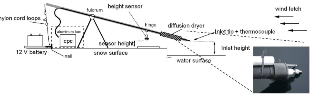
Measurements were conducted from a three meter long rod positioned on a tripod (acting as the fulcrum) so that the user could lift an aerosol inlet to fixed heights while remaining at a distance downwind to prevent contamination (Fig. 1). On
the user side of this gradient pole, a condensation particle counter (CPC 3010, TSI, St. Paul, MN, USA) along with a vacuum pump and laptop were placed in a small aluminum box for weather protection, and to preserve the small amount of heat produced by the instruments. A 12-volt battery placed outside the box was connected to a 12 VDC/220 VAC con-verter to supply the power needs of all instruments. The bat-tery also stabilized a wooden board with four nails in the hor-izontal direction providing hooks for loop-knots which were tied into a nylon cord attached to the end of the rod. The loops allowed for repeatable accuracy (±1 cm) in positioning the inlet tip at a new height which was necessary to duplicate a height step-series above the ground.
A 30 cm long diffusion dryer was mounted at the entrance of the inlet to remove water from the aerosol to improve the transmission efficiency. This was especially a concern in high relative humidity conditions where particles might ex-perience a temperature difference in the sampling line and grow by condensation. Following the dryer, the aerosol sam-ple traversed the rod through a straight 2.5 m long 0.25 inch copper tube. To allow for the vertical movement of the pole, flexible conductive tubing connected the copper tube to the CPC. A critical orifice inside the CPC controlled the aerosol flow to 1 l min−1. The total aerosol transit time from inlet to counter was approximately three seconds. The CPC 3010 used in this study for the gradient system had a lower 50 % cutoff diameter at 11 nm and an upper cutoff diameter of ap-proximately 2.5 µm. The counts from the CPC were averaged and recorded every second with a laptop.
A thermocouple (Schuricht type 212, sensitivity of
±0.01 K) was used to measure the temperature directly next to the inlet tip. The thermocouple consisted of two very thin type-k wires tied together for rapid response. The analog sig-nal from the temperature probe was sent via a sheathed cable to an analog/digital converter and sampled at approximately 10 Hz to record an average every 0.5 s.
Fig. 1. Schematic of the gradient pole to measure particle number concentration and temperature profiles above snow and water surfaces. The pole is lifted up and down on the user side so that the inlet can return to various fixed heights above the surface.
2.2 Eddy covariance method
An eddy covariance (EC) system was set up on the edge of the lead approximately 300 m from the gradient pole, di-rectly measuring turbulent fluxes of sensible and latent heat and aerosol number concentrations at a height of 2.5 m (Held et al., 2011). The system consisted of a Gill R3 sonic anemometer (Gill, Lymington, UK) for three-dimensional wind measurements, a Licor LI-7500 open path analyzer (Licor, Lincoln, NE, USA) for carbon dioxide (CO2) and water (H2O) vapor concentration measurements, and a con-densation particle counter CPC 3760A (TSI, St. Paul, MN, USA) for particle number measurements. The CPC 3760A has a nominal lower cutoff diameter of 11 nm and an upper cutoff diameter of approximately 3 µm.
Turbulent fluxes were calculated according to standard eddy covariance procedures in 30 min averaging periods af-ter rotation of the turbulent winds into a streamline coor-dinate system using the planar fit method (Wilczak et al., 2001) and linear detrending. Due to the traveling time of the aerosol sample from the sampling point through the inlet tubing to the particle counter, and the traveling time in the particle counter, a constant time lag of 2.6 s was applied to synchronize the wind and the aerosol time series. The sam-pling line degraded the response time of the particle counter with regard to ambient concentration changes. It is important to bear in mind that this eddy covariance setup cannot re-solve 10 Hz aerosol number concentration fluctuations. With an estimated response time of 1.4 s and typical wind speeds of less than 4 m s−1, we found the underestimation of the aerosol fluxes due to fluctuation dampening to be less than 20 % for this study using the approach by Horst (1997). No additional corrections were applied. After calculating the tur-bulent aerosol number fluxes by eddy covariance, the deposi-tion velocityvdwas derived by normalizing the fluxFcwith
the number concentrationc, i.e.vd=−Fcc−1. The negative sign is convention to obtain positive deposition velocities in case of aerosol deposition fluxes directed towards the sur-face. The eddy covariance results given in this work are for the 30 min averaging period encompassing the sampling time of the gradient pole, or the median value of the eddy covari-ance averaging periods encompassing the gradient pole sam-pling period.
3 Sampling methodology
The gradient pole was deployed for eight days within the pack ice area (24 August to 1 September 2008) during the ASCOS expedition when the icebreaker Oden was moored to an ice floe in the Arctic Ocean. The full drift lasted from 12 August to 1 September 2008. During these 21 days the ice floe drifted slowly west- and southward about the co-ordinates 2◦–10◦W and 87◦–87.5◦N. Upon arrival, the ice surface was composed of loose granular snow and covered by a large number of melt ponds. The larger ice floes were separated by open ocean leads. Ice algae were often visible below the ice. Our initial goal with the gradient pole was to detect particle number concentrations directly over the water surface of the lead.
Fig. 2.Temperature data acquired with the gradient pole on 31 Au-gust over the frozen lead:(a)measurement height [cm],(b) temper-ature [◦C],(c)normalized temperature [K].
of the ship. The lead itself was located approximately 3 km away from the ship. During the measurement period, the total particle number concentrations measured with the CPC were all below 100 cm−3, and decreased progressively to values below 10 cm−3.
4 Data analysis
4.1 Temperature profiles
It was necessary to develop a standard method to consis-tently analyze all raw data collected by the gradient pole. The analysis procedure is presented here with examples for temperature and concentration data. Figure 2a and b shows raw height and temperature profiles collected over the Arc-tic pack ice on 31 August 2008. The triangular patterns in Fig. 2a show a series of up and down height traces of the in-let. The inlet was held at each step for approximately 20 s before changing to the next height. The small spikes seen on the height steps are due to overshoot of the pole.
To consider the measured temperature changes due to vari-ations in the inlet height only, it was necessary to remove the slower temperature trends. For each measurement run, a rolling boxed-median of 1500 data points (∼15 min) shown as a dotted line in Fig. 2b was subtracted from the raw data. By subtracting the baseline from the raw data, the normalized temperature trace centered at 0◦C is produced (Fig. 2c).
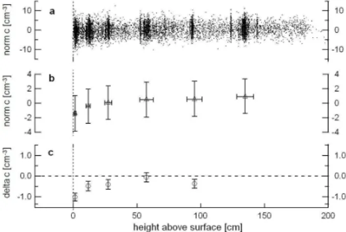
With the slower ambient temperature trend removed, the normalized temperature data plotted directly against the in-let height revealed groups of temperature points at each level (Fig. 3a). Each of these groups of data points was averaged and the means are plotted in Fig. 3b with the respective stan-dard deviations as the error bars. Since the error bars for some data points overlap with others, we first determined whether the mean data points are significantly different from
Fig. 3.Significance of temperature gradient in profile data:(a) indi-vidual data points of normalized temperature,(b)normalized tem-perature averaged at each height with the standard deviations as the error bars, and(c)the difference between adjacent means from left to right with±twice the standard errors as the error bars.
one another. If we take the difference between adjacent pairs of mean temperatures from left to right, we produce the data points in Fig. 3c. The error bars in Fig. 3c are derived from the standard error SE of the difference between two adjacent means,
SE=
s
σ12
(N1−1)+
σ22
(N2−1)
, (1)
whereσ1andσ2are the respective standard deviations, and
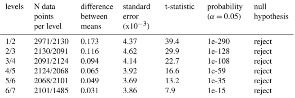
N1andN2are the number of measured data points. In com-mon practice, the 95 % confidence interval is obtained by tak-ing twice the standard error (Lanzante, 2005), shown as error bars in Fig. 3c. If twice the standard error is greater than the difference, then the error bar will cross zero and the two mean data points are considered “not significantly different”. In the case shown in Fig. 3c, the error bars for all adja-cent mean pairs do not cross zero. For the sake of complete-ness, we extend the analysis one step further by applying an independent two-tailed T-test to each pair of mean val-ues. Closely related, the t-value is the difference between two means divided by the standard error. Table 1 shows the t-values and the probabilities to not reject the null hypothe-sis (that two points are statistically the same) for a common, yet arbitrary significance levelα= 0.05. The null hypothesis is rejected for all data pairs, and therefore we conclude that the adjacent data points are significantly different, despite the overlapping standard deviations.
Table 1.T-test results for adjacent means of the temperature profile on 31 August.
levels N data points per level
difference between means
standard error (x10−3)
t-statistic probability (α=0.05)
null hypothesis
1/2 2/3 3/4 4/5 5/6 6/7
2971/2130 2130/2091 2091/2124 2124/2068 2068/2101 2101/1485
0.173 0.116 0.094 0.065 0.049 0.031
4.37 4.62 4.14 3.92 3.69 3.86
39.4 29.9 22.7 16.6 13.2 7.9
1e-290 1e-128 1e-108 1e-59 1e-35 1e-15
reject reject reject reject reject reject
negative for all pairs. It should be stressed that a profile mea-surement may still be perfectly valid without satisfying these criteria. In particular, criterion (1) is simply an indication that the differences between two heights could be resolved by our measurements. Under neutral conditions or for closer spaced measurement levels, this criterion will eventually not be met.
4.2 Aerosol concentration profiles
In Fig. 4, particle number concentration data collected with the gradient pole over the Arctic pack ice on 28 August are presented. We choose this example because it illustrates a weak gradient that was resolved despite the large variability in the particle counts. For consistency, we take the same data approach as for the temperature case. Fig. 4a displays the height profiles, which appear less uniform than in the tem-perature case discussed above. The irregularity in the profiles was present in the beginning stages of the experimental runs due to lack of practice with raising and lowering the gradi-ent pole and struggling with initial adjustmgradi-ents of the setup in the cold conditions. As can be seen in the latter part of the measurement period, we also tried faster scanning of the profiles, but the results provided poor averaging statistics.
Figure 4b displays the particle number concentration recorded every second. Despite the natural short-term fluc-tuations which are on the order of 10 particles cm−3, a weak gradient can be discerned which tracks the changes in height. As previously done for the temperature case, a median base-line is subtracted from the raw data producing the normalized data in Fig. 4c.
The profile extracted from the normalized data is shown in Fig. 5. Because of the data scatter due to the non-uniform height levels, we show both the time and height standard de-viations in the groups of points which are averaged. Using the standard error method, the differences between the four data points that are resolved nearest to the surface in Fig. 5c are consistent in their sign of gradient, and thus confirm the existence of a valid gradient. The T-test results (Table 2) show that the null hypothesis is rejected for all data pairs
ex-Fig. 4. Particle concentration data acquired with the gradient pole on 28 August over the snow surface:(a)measurement height [cm], (b)particle concentration [cm−3],(c)normalized particle concen-tration [cm−3]. A total of 7 scans began at 14:20 (initial data not shown), with an average sampling time per height level = 20 s. Av-erage data points per height level = 1200.
cept the pair of data points 4 and 5. This indicates that adja-cent data points (except data points 4 and 5) are significantly different.
4.3 Flux-profile relationships
In a layer near the surface, turbulent fluxes are considered to be constant with height. Thus, vertical fluxes and gradients may be related using Monin-Obukhov similarity theory in this so-called constant flux layer (cf. Kaimal and Finnigan, 1994; Foken, 2008). For the turbulent fluxes of momentum and sensible heat,FmandFh, we obtain
Fm=u′w′= −Km
∂U
∂z, (2)
Fh=w′T′= −Kh
∂T
∂z, (3)
Table 2.T-test results for adjacent means of the aerosol concentration profile on 28 August.
levels N data points per level
difference between means
standard error (x10−3)
t-statistic probability (α=0.05)
null hypothesis
1/2 2/3 3/4 4/5 5/6
1220/821 821/537 537/939 939/435 435/1110
−1.0115 −0.4824 −0.4063 −0.0570 −0.3666
0.137 0.164 0.165 0.172 0.169
−10.7 −4.03 −3.52 −0.50 −3.34
1e-26 1e-05 3e-04 0.620 0.001
reject reject reject do not reject reject
Average sample time per level = 844 s or 14.1 min.
Fig. 5. Significance of particle number gradient in profile data:(a)individual data points of normalized particle number con-centration,(b)normalized particle number concentration averaged at each height with the standard deviations as the error bars, and (c)the difference between adjacent means from left to right with± twice the standard errors as the error bars.
temperature,Uis the wind speed [m s−1],T is the tempera-ture [K], andzis the measurement height [m].
Kis the eddy diffusivity,
Km,h=
kzu∗ φm,h(z/L)
, (4)
wherekis the von Karman constant (= 0.40),u∗is the fric-tion velocity [m s−1], and subscripts m and h refer to mo-mentum and sensible heat, respectively. φm,h(z/L) are the corresponding stability correction functions
In the literature, values between 1.0 and 1.39 are reported for the ratioKh/Km (which is the inverse of the turbulent Prandtl number, e.g. Foken, 2008). Values larger than unity imply that heat transport is more effective than momentum transport. For reasons of simplicity, we will use a value of unity, thusKh=Km.
Fig. 6.Probability density function of the stability parameterz/L, based on the whole ASCOS measurement period near the lead.
The stability functions for the fluxes of momentum and sensible heat,φmandφh, depend only on the dimensionless height,z/L,whereLis the Obukhov length,
L= − u
3 ∗ kTg
0w
′T′, (5)
gis the gravitational acceleration (= 9.81 m s−2), andT0is a reference temperature.
The stability correction functions are determined empir-ically, and many different formulations for the functional shape ofφhave been suggested in the literature (e.g. Dyer, 1974; Businger, 1988). For neutral stratification, i.e.z/L= 0, the stability correction functions are unity by definition,
Using these simplifications and integrating Eq. (3) be-tween the two heightsz1andz2, we arrive at
T2−T1= −
Fh
u∗kln
z
2
z1
. (6)
The sensible heat flux indicates a positive (upward) flux of sensible heat whenT2< T1, and vice versa. Strictly speak-ing, Eq. (6) is only true for potential temperature. In this study performed in the lowest 2 m of the boundary layer at sea level, we used the differences of actual air temperature at two heights as a good approximation of the differences of potential temperature at these two heights. It should be kept in mind that the difference between actual and potential tem-perature increases with height, thus introducing a small bias to the temperature difference. For a pressure drop of roughly 0.143 hPa m−1, a typical temperature of 273 K, and a typical pressure of 1013 hPa we obtain a change in temperature of 0.022 K between the surface and a height of 2 m.
We can also derive the relationship of the particle number concentration profile and the particle number flux,
c2−c1= −
Fc
u∗kln
z
2
z1
, (7)
wherec1andc2are the particle number concentrations in the measurement heightsz1andz2, andFcis the particle num-ber flux. Again, we assume the turbulent eddy diffusivity for particle number,Kc=Km, and the stability correction func-tion for the particle number flux,φc(0) = 1. It should be em-phasized that the theoretical assumptions underlying Eq. (7), i.e. Monin-Obukhov similiarity theory, have not been vali-dated for atmospheric aerosols. However, our aerosol data show consistency with the logarithmic profile of Eq. (7), whereas a widely used equation for the theoretical form of aerosol concentration above a surface source (e.g. Fairall et al., 2009),
cz=ch
z
h
vg u∗k
, (8)
withcz being the aerosol concentration at height z, ch be-ing a reference concentration at an arbitrary heighth, and
vgthe gravitational settling velocity, cannot explain the ob-served concentration differences. We note that Eq. (8) de-pends strongly on vg; during ASCOS, the portion of the aerosol spectrum sampled by the CPC was dominated by sub-100 nm particles. This is consistent with previous ob-servations of a distinct Aitken mode in the Arctic aerosol (e.g. Covert et al., 1996; Leck and Bigg, 2005b). For such small particles, vg is negligibly small, and turbulent parti-cle fluxes will behave similar to other scalar fluxes. Andreas et al. (2010) use the exponent of Eq. (8), vg/u∗k, to iden-tify the dominant process, gravitational settling or turbulent mixing. For typicalu∗= 0.1 m s−1and a particle diameter of 100 nm, we find an exponent of∼3×10⁻⁵, while for a par-ticle diameter of 5 µm, the exponent is roughly 0.03. Thus,
for our conditions, turbulent mixing clearly dominates over gravitational settling, which is not the case for supermicron particles.
Equations (6) and (7) allow us to calculate the sensible heat flux,Fh, and the particle number flux,Fc, from gradi-ents of temperatureT and particle number concentrationc, provided that the value of the friction velocity,u∗, is known. In the present case, we have independent information ofu∗, and also of sensible heat and aerosol flux, from simultaneous eddy covariance flux measurements.
If we presume that our temperature data behave accord-ing to Eq. (6), then we can plot the temperature differences (T2−T1)against the logarithmic height ratio ln(z2/z1)and produce a linear plot with a slope that equals−Fh(u∗k)−1. If we obtainu∗from the eddy covariance data, we can solve for the heat fluxFh from the slope of a linear regression. Likewise, the same can be done for the particle concentration data using Eq. (7), solving forFc. We acknowledge ongoing discussions about the appropriate value of the von Karman constantkin the case of particle concentration (Petelski and Piskozub, 2006, 2007; Andreas, 2007). However, our data are too limited to contribute to this discussion, and we pro-ceed with a value ofk=0.40.
It should be pointed out that the slope of the linear regres-sion for Eqs. (6) and (7), and thus the flux estimateFhand
Fc, is identical to the slope derived from the more standard approach of analyzing flux-profile relationships, i.e. fitting a least-squares relation between ln(z) andT orc, respectively.
4.4 Flux estimates from profile measurements
We will now illustrate two examples using the above equa-tions to solve for the sensible heat fluxFhand the particle number flux Fc. For the case ofFh, we take profile data from a period on 31 August (31/08a) and plot the tempera-ture differences (T2−T1)between the height levels on the vertical axis and ln(z2/z1)on the horizontal axis to produce Fig. 7a. In this particular case on 31 August, the gradient pole was used to measure the temperature at seven height levels above the frozen lead. Using all possible combina-tions of temperature differences between seven height lev-els yields 6 + 5 + 4 + 3 + 2 + 1 permutations of (T2−T1)or 21 data points.
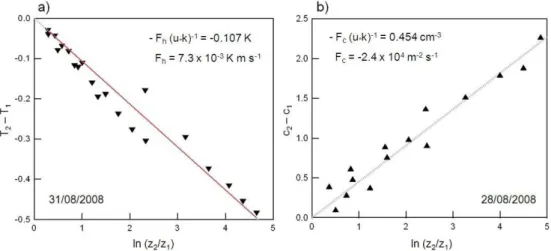
Fig. 7.Estimation of(a)the sensible heat fluxFhon 31 August and(b)the particle number fluxFcon 28 August from a linear regression of the temperature and particle concentration profiles according to Eqs. (6) and (7), respectively.
evidence for this, and by keeping all data intact in the figure, we gain insight into the variability of the data with respect to the logarithmic behavior.
The surface layer similarity theory, from which this be-havior arises, is strictly valid only for measurement heights much larger than the roughness lengthz0. Values ofz0over summer sea ice are given in the literature as typically 10−5to 10−2m (Held et al., 2011; Persson et al., 2002; Tjernstr¨om, 2005). Thus, the presented measurements should be valid down to a few centimeters above the surface.
A linear regression fit to the data in Fig. 7a yields a slope of −0.107 with a coefficient of determination, R2=0.98. Setting the slope equal to −Fh(u∗k)−1 yields a kinematic sensible heat fluxFh= 7.3×10⁻³K m s−1. This is a posi-tive value, indicating that the heat flux is upward and that the surface behaves as a heat source. We obtain the sensi-ble heat fluxH in dynamic units [W m−2] by multiplying the sensible heat flux in kinematic units [K m s−1] by the product of the air density,ρair= 1.225 kg m−3, and the spe-cific heat of air,cp= 1004 J kg−1K−1. In this case we obtain
H=8.9 W m−2. This is in good agreement with the sensi-ble heat flux obtained from eddy covariance measurements,
H=6.7 W m−2.
We now demonstrate the same approach for particle num-ber data measured on 28 August over the snow surface. Figure 7b shows the particle number concentration differ-ences (c2−c1)plotted against the respective height ratios ln(z2/z1). The regression line has a slope of +0.454 with
R2=0.98. When set equal to−Fc(u∗k)−1, we obtain a par-ticle number flux of−2.4×10⁴m−2s−1. The negative value indicates particle deposition. The particle number concentra-tion decreased towards the surface also indicating an aerosol sink. Finally, we obtain the particle deposition velocity by normalizingFcwith the ambient particle number concentra-tionc,vd=Fcc−1, herevd=0.38 mm s−1.
To provide clarity to the outlined procedures, we briefly recap what has been done. First, the raw temperature and aerosol concentration data measured with the gradient pole was normalized to create an average data set as a function of height. Second, a linear method of standard errors was applied to the averaged data for each date to determine if an observed gradient was significant. Third, the same averaged data were plotted for each date according to a theoretical flux-profile relationship to extract a slope andR2value from a linear regression. In contrast to the standard error method, the coefficients of determination, R2, signify how well the data conform to the logarithmic model. For the data sets that showedR2>0.5, the sensible heat fluxH(grad)and de-position velocityvd(grad) were calculated, with the subscript “grad” referring to the gradient pole.
5 Results and discussion
5.1 Sensible heat flux estimates
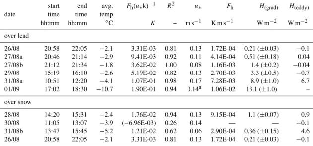
We apply the approach introduced in Sect. 4.4 to all temper-ature measurements by obtaining fits to the data outlined in Table 3. The first four columns summarize the measurement dates, start and sampling times, and average temperatures en-countered. The next three data columns summarize the slope parametersFh(u∗κ)−1, the coefficients of determination,R2, and the friction velocity,u∗, taken from simultaneous eddy covariance measurements (Held et al., 2011).FhandH(grad) were calculated only for cases when R2>0.50; thus, the temperature gradient on 30 August was excluded.
Table 3. Summary of temperature slope parameters, kinematic sensible heat fluxFh, and dynamic sensible heat fluxH over the lead and snow surfaces; values in parentheses are discarded due to rejection by standard errors or by low coefficients of determinationR2.
start end avg. Fh(u∗k)−1 R2 u∗ Fh H(grad) H(eddy) date time time temp
hh:mm hh:mm ◦C K – m s−1 K m s−1 W m−2 W m−2
over lead
26/08 20:58 22:05 −2.1 3.31E-03 0.81 0.13 1.72E-04 0.21 (±0.03) −0.1 27/08a 20:46 21:14 −2.9 9.41E-03 0.92 0.11 4.14E-04 0.51 (±0.18) 0.04 27/08b 21:12 21:34 −1.8 3.62E-02 1.00 0.08 1.16E-03 1.4 (±0.2) −0.04 29/08 15:19 16:10 −2.6 5.19E-02 0.82 0.13 2.70E-03 3.3 (±0.5) −0.7 31/08a 10:51 12:20 −4.1 1.07E-01 0.98 0.17 7.28E-03 8.9 (±1.0) 6.7 01/09 17:02 18:30 −10.7 1.90E-01 0.94 0.14a 1.06E-02 13.1 (±1.0) –
over snow
28/08 14:20 15:31 −2.4 1.76E-02 0.94 0.13 9.15E-04 1.1 (±0.07) 0.9 30/08 11:05 13:07 −3.9 (−6.96E-03) 0.26 0.14 — — −0.1 31/08b 13:47 15:45 −5.2 1.21E-02 0.62 0.06 2.90E-04 0.36 (±0.15) 4.6 26/08 20:58 22:05 −2.1 3.31E-03 0.81 0.13 1.72E-04 0.21 (±0.03) −0.1
au
∗estimated since there were no flux data.
ambient temperatures rapidly below −10◦C and the mea-sured temperature profile indicated a sensible heat flux of 13.1 W m−2.
Over the snow surface, however, weaker temperature pro-files dominated. The lead/snow contrast was especially evi-dent during measurements made on 31 August, first over the frozen lead (31/08a) and then over the snow surface (31/08b). The rather robust profile over the lead (R2=0.98) was fol-lowed by a close to non-detectable profile over the snow (R2=0.62). Over the lead, a gradient corresponding to a sensible heat flux ofH=8.9 W m−2 may be expected due to the difference between the average air temperature (in this case−4.1◦C) and the average temperature of the Arctic wa-ters of−1.8◦C. In contrast, the snow surface covers a two to three meter thick layer of pack ice, and apart from being far more insulated from the ocean waters, has a lower thermal conductivity. The air temperature dropped from−4.1◦C dur-ing the lead measurements to−5.2◦C during the snow sur-face measurements, while the observed profile corresponds with a rather low sensible heat flux ofH=0.4 W m−2.
The heat flux values in this work (gradient pole 0.2 to 13.1 W m−2; eddy covariance
−0.1 to 6.7 W m−2)fall within the range of previous measurements in Arctic summertime. Several heat flux measurements have been reported over the Arctic. For example, Persson et al. (2002) reported an av-erage sensible heat flux between 3 and 4 W m−2 from Au-gust to September on ice floes in the Beaufort and Chukchi Seas as part of the SHEBA field experiment. They also re-ported 5 W m−2as the maximum in the average diurnal sen-sible heat flux for the month of August. During ASCOS, the sensible heat flux showed large variability with mean val-ues ranging from−2 to 6 W m−2 (Sedlar et al., 2010). In
winter, Andreas et al. (1979) found sensible heat fluxes over Arctic leads one to two orders of magnitude larger (∼100– 500 W m−2)than in this summertime study.
5.2 Particle number flux estimates
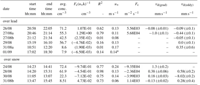
Table 4. Summary of particle concentration slope parameters, aerosol number fluxFc, and deposition velocityvdover the lead and snow surfaces; values in parentheses are discarded due to rejection by standard errors or by low coefficients of determinationR2.
start end avg. Fc(u∗k)−1 R2 u∗ Fc vd(grad) vd(eddy) date time time conc.
hh:mm hh:mm cm−3 cm−3 - m s−1 m−2s−1 mm s−1 mm s−1
over lead
26/08 20:58 22:05 71.2 1.07E-01 0.62 0.13 5.56E03 −0.08 (±0.01) −0.09 (±0.1) 27/08a 20:46 21:14 55.3 1.29E+00 0.79 0.11 5.68E04 −1.0 (±0.1) −0.44 (±0.1) 27/08b 21:12 21:34 42.5 (2.35E-02) 0.01 0.08 – – −0.05 (±0.1) 29/08 15:19 16:10 56.7 (−4.76E-02) 0.16 0.13 – – 0.0 (±0.1) 31/08a 10:51 12:20 8.6 (1.90E-03) 0.01 0.17 – – 0.35 (±0.6) 01/09 17:02 18:30 7.9 (−6.50E-03) 0.14 0.14a – – –
over snow
24/08 14:23 14:41 72.4 −9.74E-01 0.77 0.24 −9.35E04 1.3 (±0.2) – 28/08 14:20 15:31 61.9 −4.54E-01 0.98 0.13 −2.36E04 0.38 (±0.06) 0.58(±0.2) 30/08 11:05 13:07 22.3 −7.12E-02 0.75 0.14 −3.99E03 0.18 (±0.03) −8.02(±0.2) 31/08b 13:47 15:45 8.51 4.73E-02 0.73 0.06 1.14E03 −0.13 (±0.02) 0.28(±0.4)
au
∗estimated since there were no flux data.
one measurement would be unreliable. Also important to consider are the lower ambient particle number concentra-tions (less than 60 cm−3) measured after the transition on 27 August which made surface sinks harder to detect. In con-trast, the detection of weak surface sources would be aided by the low ambient concentrations but were not observed either.
For the strongest source profile on 27 August (27/08a), the calculated particle number flux isFc=5.68×10⁴ particles m−2s−1. Converting units this corresponds with a net emis-sion of approximately 340 particles cm−2min−1. If we as-sume a 100 m mixing depth, a reasonable height for the cen-tral Arctic boundary layer (Tjernstr¨om, 2005), and a 15 min residence time of an air parcel over open water, then the net change in particle concentration would be approximately 0.5 particles cm−3h−1, without considering sink mechanisms.
If we compare this number to the range of variability in particle number concentrations that were observed, it will give us an idea of how the source might impact the aerosol population. We estimate from the CPC observations that the particle variability ranged from 20 to 100 cm−3h−1 for ambient particle concentrations between 0.1 and 100 cm−3. Therefore, an aerosol source on the order of 0.5 cm−3h−1 might only be observed under stable conditions with low par-ticle concentrations; in most other cases, it may be consid-ered negligible.
Particle profiles over the snow covered ice surface showed a different behavior. On 24, 28, and 30 August, the results imply an aerosol sink at the surface. One inconsistent pro-file occurred on 31 August (31/08b), where the trend was opposite and implied a weak source. The values of the
calcu-lated deposition velocities are in good agreement with previ-ous measurements of particle number fluxes over snow sur-faces and in the Arctic. Duan et al. (1988) report values of
vd=0.34 mm s−1 over snow for particles in the size range from 0.15 to 0.3 µm. Bergin et al. (1995) derived deposi-tion velocities of particulate sulfate ranging fromvd=0.23 to 0.62 mm s−1 using surrogate surfaces and impactor data. Gr¨onlund et al. (2002) found slightly higher transfer veloc-ities of 0.8 to 18.9 mm s−1 using a condensation particle counter and eddy covariance over snow. In the high Arctic, Nilsson and Rannik (2001) report median deposition veloci-tiesvd=0.26 mm s−1over ice andvd=0.40 to 0.73 mm s−1 towards open leads. They also observed emission fluxes on the same order of magnitude. During ASCOS, Held et al. (2011) observed particle deposition values ranging from 0.27 to 0.68 mm s−1during deposition-dominated periods.
5.3 Intercomparison with eddy covariance measurements
Finally, the flux estimates calculated from the gradient pole are compared with direct eddy covariance flux measurements by Held et al. (2011).
values for the gradient pole data are fairly good for nearly all profiles (with the exception of 30/08), and apart from any fitting, the existence of temperature gradients is evident in the raw gradient pole data, as shown for example in Fig. 3. It must be kept in mind that the eddy covariance flux de-rived from the sonic temperature fluctuations is not the sen-sible heat flux but close to the buoyancy flux. However, An-dreas et al. (2005) demonstrated that for typical polar condi-tions (low temperature, and hence low absolute humidity) the sonic temperature flux is a very good approximation to the sensible heat flux. It should also be noted that the eddy co-variance system was located approximately 300 m from the gradient pole, and although we designed the experiments in a way that the air trajectories from over the lead or the snow surface were the same for both systems, it is certain that the actual surface footprint was different for the two measure-ments. This could also be due to the height difference be-tween the two measurements: the eddy covariance system located at 2.5 m above ground could reasonably be decou-pled from the 1.5 m surface layer in which the gradient pole was deployed. Rapid changes in the magnitude and direction of the flux, for example, could localize the measurements, producing converging and diverging flux profiles with height. However, turbulence measurements at various heights during ASCOS do not provide evidence for decoupled layers.
Nevertheless, we also compare the particle deposition ve-locities,vd(grad)andvd(eddy), in Table 4. There are two parti-cle source cases over the lead before freeze-up, and two sink cases over the snow covered ice surface (24/08 and 28/08) that show good agreement. The low R2 value on 24 Au-gust is likely due to the low number of data points since only two profiles were measured with the gradient pole. For the transitional day when the lead froze on 27 August,vd(eddy) also indicates a transition in the same direction as data col-lected with the gradient pole. A change in vd(eddy) from
−0.44 mm s−1to−0.05 mm s−1is consistent with the shut-down of a particle source at the lead, indicated by a change invd(grad) from−1.0 mm s−1to a situation without any de-tectable profile.
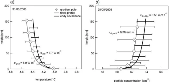
In order to visualize these results, we construct profiles corresponding with the eddy covariance data and compare them directly against the profiles measured with the gradient pole. In Fig. 8a, we continue with the case shown in Fig. 7a (31/08a). First, we use the slope calculated from the gradient pole data in Fig. 7a, and extend the logarithmic curve from the temperature measured at the lowest height. The uncer-tainty shown is the standard deviation determined for each data point. As one would expect for a goodR2value, the reconstructed profile (grey line) passes fairly well through the data points. The black curve in Fig. 8a is the profile de-rived from the eddy covariance flux measurement extrapo-lated down to the same reference temperature at surface level. The error bars indicate the estimated uncertainties in the sen-sible heat flux, taken as 20 % in the eddy covariance mea-surements (Foken, 2008). The constructed eddy covariance
profile is consistent with a sensible heat flux of 6.7 W m−2 which is slightly smaller but on the same order as the gra-dient measurement of 8.9 W m−2, and within the estimated uncertainties of the flux values.
For the aerosol concentration profiles, we extend the ex-ample of 28 August in Fig. 8b and compare the aerosol pro-file from the gradient data with the propro-file consistent with the eddy covariance measurements. The uncertainty of the reconstructed profile (grey line) is the standard deviation de-termined for each data point. The two profiles seen in Fig. 8b can be considered in reasonable agreement, however with a large uncertainty. In this case, the deposition velocity from the gradient measurements vd(grad)=0.38 mm s−1 is com-pared against vd(eddy)=0.58 mm s−1. The agreement be-tween the two curves appears reasonable and just contained within the uncertainty of the eddy covariance measurement due to particle counting statistics indicated by the error bars of the black curve. The uncertainty of the deposition velocity
1vdwas calculated after Fairall (1984) by
1vd=
σw
√
N, (9)
whereσwis the standard deviation of the vertical wind speed, andN is the total number of particles counted during the averaging interval of 30 min.
6 Conclusions
A gradient pole was deployed over the Arctic pack ice area at about 87◦N to measure temperature and particle number concentration profiles in height steps varying from 1–2 cm up to 1.5 m above the surface. Nearby, a sonic anemometer and particle counter at a height of 2.5 m were used to directly measure the sensible heat and particle number fluxes by eddy covariance. The results were compared over the snow cov-ered pack ice, and over the open and frozen lead. In the time period of deployment (24 August to 1 September), the open lead froze, ambient temperatures dropped, and particle num-ber concentrations decreased from around 100 cm−3to be-low 10 cm−3.
The sensible heat flux and particle deposition velocity were calculated from the gradient pole data by applying a lin-ear regression to the data assuming it followed a logarithmic profile. The logarithmic behavior of the data was confirmed for all cases where an obvious trend was seen, as indicated by theR2values.
In nearly all cases, the ambient temperatures measured with the gradient pole increased towards the surface, giving positive heat flux values. The strongest temperature gradients were measured after the open lead froze on 27 August. The corresponding sensible heat fluxes reached maximum values of 8.9 and 13.1 W m−2over the lead.
Fig. 8.Intercomparison of profiles fitted to the gradient pole data (grey) and profiles consistent with the simultaneous eddy covariance flux measurement (black).(a)Temperature profiles on 31 August, and(b)particle concentration profiles on 28 August.
emission in two measurements over the open lead which was confirmed by eddy covariance measurements. No reliable particle number profiles of any sort were detected over the frozen lead. The snow surfaces behaved in general as par-ticle sinks with deposition velocities ranging from 0.18 to 1.3 mm s−1 by the gradient method, and ranging from 0.28 to 0.58 mm s−1by eddy covariance. These findings corrobo-rate the original hypothesis that open leads can act as particle sources.
An operational shortcoming of the gradient pole as pre-sented in this study lies in the manual control of heights and timing. Therefore, the data collection can only be a snap-shot representation of the atmospheric conditions, in contrast to continuous monitoring with the eddy covariance system. However, its simplicity in construction and profile acquisi-tion might offer advantages, for example as an alternative to more expensive and complicated eddy covariance systems. Also, the capability to carry out measurements very close to the surface is beneficial.
Although the gradient pole method is an indirect way to calculate the flux, it appeared to reveal strong gradients even when the eddy covariance data were ambiguous. This was already observed in the raw data. However, it has to be kept in mind that the estimated flux values presented in this study rely on the knowledge ofu∗from an independent measure-ment (with a flux footprint different from the gradient pole footprint). A reliable estimate of the friction velocity is al-ways required. Without turbulence measurements,u∗ may be parameterized using a wind speed measurement while es-timating the surface roughness. With wind speed measure-ments at two or more heights, the friction velocity and the roughness can (in theory) be estimated directly.
Finally, the gradient pole method may be extended by adding, for example, a fast scanning mobility particle sizer for size-resolved particle measurements, a humidity sensor, or aerosol and trace gas analyzers. Further improvements such as an integrated data acquisition system and a fully au-tomated inlet height control will make the presented setup even more practical in future studies.
Acknowledgements. This work is part of ASCOS (the Arctic Sum-mer Cloud-Ocean Study) and was funded by the German Research Foundation No. HE939/29-1. AH was supported by the Bert Bolin Center for Climate Research at Stockholm University. PV was supported by the Finnish Cultural Foundation, Lapland Regional fund. ASCOS was made possible by funding from the Knut and Alice Wallenberg Foundation, the Swedish Research Council and the DAMOCLES European Union 6th Framework Integrated Research Project. The Swedish Polar Research Secretariat (SPRS) provided access to the icebreaker Oden and logistical support. We are grateful to the Swedish Polar Research Secretariat logistics staff and to Oden’s captain Mattias Peterson and his crew. ASCOS is an IPY project under the AICI-IPY umbrella and is an endorsed SOLAS project. Thanks are due to Jost Heintzenberg and David Covert for an endless exchange of ideas.
Edited by: I. Brooks
References
Aller, J. Y., Kuznetsova, M. R., Jahns, C. J., and Kemp, P. F.: The sea surface microlayer as a source of viral and bacterial enrich-ment in marine aerosols, J. Aerosol Sci., 36, 801–812, 2005. Andreas, E. L: Comment on “Vertical coarse aerosol fluxes in the
Andreas, E. L., Paulson, C. A., Williams, R. M., Lindsay, R. W., and Businger, J. A.: The turbulent heat flux from Arctic leads, Bound. Lay. Meteorol., 17, 57–91, 1979.
Andreas, E. L., Paulson, C. A., and Williams, R. M.: Observa-tions of condensate profiles over Arctic leads with a hot-film anemometer, Q. J. Roy. Meteorol. Soc., 107, 437–460, 1981. Andreas, E. L., Jordan, R. E., and Makshtas, A. P.: Parameterizing
turbulent exchange over sea ice: The ice station Weddell results, Bound. Lay. Meteorol., 114, 439–460, 2005.
Andreas, E. L., Jones, K. F., and Fairall C. W.: Production ve-locity of sea spray droplets, J. Geophys. Res., 115, C12065, doi:10.1029/2010JC006458, 2010.
Bergin, M. H., Jaffrezo, J.-L., Davidson, C. I., Dibb, J. E., Pandis, S. N., Hillamo, R., Maenhaut, W., Kuhns, H. D., and Makela, T.: The contributions of snow, fog, and dry deposition to the summer flux of anions and cations at Summit, Greenland, J. Geophys. Res., 100, 16275–16288, 1995.
Bezdek, H. F. and Carlucci, A. F.: Concentration and removal of liquid microlayers from a seawater surface by bursting bubbles, Limnol. Oceanogr., 19, 126–132, 1974.
Bigg, E. K. and Leck, C.: The composition of fragments of bubbles bursting at the ocean surface, J. Geophys. Res., 113(D1), 1209, doi:10.1029/2007JD009078, 2008.
Bigg, E. K., Leck, C., and Tranvik, L.: Particulates of the surface microlayer of open water in the central Arctic Ocean in summer, Mar. Chem., 91, 131–141, 2004.
Blanchard, D. C.: Electrically charged drops from bubbles in sea water and their meteorological significance, J. Atmos. Sci., 15, 383–396, 1958.
Businger, J. A.: A note on the Businger-Dyer profiles, Bound. Lay. Meteorol., 42, 145–151, 1988.
Ceburnis, D., O’Dowd, C. D., Jennings, G. S., Facchini, M. C., Emblico, L., Decesari, S., Fuzzi, S., and Sakalys, J.: Ma-rine aerosol chemistry gradients: Elucidating primary and sec-ondary processes and fluxes, Geophys. Res. Lett., 35, L07804, doi:10.1029/2008GL033462, 2008.
Chin, W. C., Orellana, M. V., and Verdugo, P.: Spontaneous assem-bly of marine dissolved organic matter into polymer gels, Nature, 391, 568–572, 1998.
Covert, D. S., Wiedensohler, A., Aalto, P., Heintzenberg, J., Mc-Murry, P. H., and Leck, C.: Aerosol number size distributions from 3 to 500 nm diameter in the arctic marine boundary layer during summer and autumn, Tellus B, 48, 197–212, 1996. Duan, B., Fairall, C. W., and Thomson, D. W.: Eddy correlation
measurements of the dry deposition of particles in wintertime, J. Appl. Meteorol., 27, 642–652, 1988.
Dyer, A. J.: A review of flux-profile relationships, Bound. Lay. Me-teorol., 7, 363–372, 1974.
Fairall, C. W.: Interpretation of eddy-correlation measurements of particulate deposition and aerosol flux, Atmos. Environ., 18, 1329–1337, 1984.
Fairall, C. W., Banner, M. L., Pierson, W. L., Asher, W., and Morison, R. P.: Investigation of the physical scaling of sea spray spume droplet production, J. Geophys. Res., 114, C10001, doi:10.1029/2008JC004918, 2009.
Foken, T.: Micrometeorology, Springer, Berlin, 306 pp., 2008. Gr¨onlund A., Nilsson, D., Koponen, I. K., Virkkula, A., and
Hans-son, M.: Aerosol dry deposition measured with eddy-covariance technique at Wasa and Aboa, Dronning Maud Land, Antarctica,
Ann. Glaciol., 35A, 355–361, 2002.
Held, A., Brooks, I. M., Leck, C., and Tjernstr¨om, M.: On the po-tential contribution of open lead particle emissions to the central Arctic aerosol concentration, Atmos. Chem. Phys., 11, 3093– 3105, doi:10.5194/acp-11-3093-2011, 2011.
Horst, T. W.: A simple formula for attenuation of eddy fluxes mea-sured with first-order-response scalar sensors, Bound. Lay. Me-teorol., 82, 219–233, 1997.
Kaimal, J. C. and Finnigan, J. J.: Atmospheric boundary layer flows, Oxford University Press, New York, Oxford, 289 pp., 1994.
Kuznetsova, M., Lee, C., and Aller, J.: Characterization of the pro-teinaceous matter in marine aerosols, Mar. Chem., 96, 359–377, 2005.
Lanzante, J. R.: A cautionary note on the use of error bars, J. Cli-mate, 18, 3699–3703, 2005.
Leck, C. and Bigg, E. K.: Aerosol production over remote marine areas – a new route, Geophys. Res. Lett., 26, 3577–3580, 1999. Leck, C. and Bigg, E. K.: Biogenic particles in the surface
micro-layer and overlaying atmosphere in the central Artic ocean during summer, Tellus, 57B, 305–316, 2005a.
Leck, C. and Bigg, E. K.: Source and evolution of the marine aerosol – a new perspective, Geophys. Res. Lett., 32, L19803, doi:10.1029/2005GL023651, 2005b.
Leck, C. and Bigg, E. K.: A modified aerosol-cloud-climate feedback hypothesis, Environ. Chem., 4, 400–403, doi:10.1071/EN07061, 2007.
Leck, C. and Bigg, E. K.: Comparison of sources and nature of the tropical aerosol with the summer high Arctic aerosol, Tellus, 60B, 118–126, doi:10.1111/j.1600-0889.2007.00315.x, 2008. Leck, C. and Bigg, E. K.: New particle formation of marine
biolog-ical origin, Aerosol Sci. Technol., 44, 570–577, 2010.
Leck, C., Norman, M., Bigg, E. K., and Hillamo, R.: Chemi-cal composition and sources of the high Arctic aerosol relevant for fog and cloud formation, J. Geophys. Res., 107(D12), 4135, doi:10.1029/2001JD001463, 2002.
Nilsson, E. D. and Rannik, ¨U.: Turbulent aerosol fluxes over the Arctic Ocean: 1. Dry deposition over sea and pack ice, J. Geo-phys. Res., 106, 32125–32137, 2001.
Norris, S. J., Brooks, I. M., de Leeuw, G., Sirevaag, A., Leck, C., Brooks, B. J., Birch, C. E., and Tjernstr¨om, M.: Measurements of bubble size spectra within leads in the Arctic summer pack ice, Ocean Sci., 7, 129–139, doi:10.5194/os-7-129-2011, 2011. Persson, P. O. G., Fairall, C. W., Andreas, E. L, Guest, P. S.,
and Perovich, D. K.: Measurements near the Atmospheric Surface Flux Group tower at SHEBA: Near-surface conditions and surface energy budget, J. Geophys. Res., 107(C10), 8045, doi:10.1029/2000JC000705, 2002.
Petelski, T.: Marine aerosol fluxes over open sea calculated from vertical concentration gradients, J. Aerosol Sci., 34, 359–371, 2003.
Petelski, T. and Piskozub, J.: Vertical coarse aerosol fluxes in the atmospheric surface layer over the North polar waters of the Atlantic, J. Geophy. Res., 111, C06039, doi:10.1029/2005JC003295, 2006.
Scott, W. D. and Levin, Z.: Open channels in sea ice (leads) as ion sources, Science, 177, 425–426, 1972.
Sedlar, J., Tjernstr¨om, M., Mauritsen, T., Shupe, M. D., Brooks, I. M., Persson, P. O. G., Birch, C. E., Leck, C. Sirevaag, A., and Nicolaus, M.: A transitioning Arctic surface energy budget: the impacts of solar zenith angle, surface albedo and cloud ra-diative forcing, Clim. Dynam., online first, doi:10.1007/s00382-010-0937-5, 2010.
Tjernstr¨om, M.: The summer Arctic boundary layer during the Arc-tic Ocean Experiment 2001 (AOE-2001), Bound. Lay. Meteorol., 117, 5–36, 2005.
Wilczak, J. M., Oncley, S. P., and Stage, S. A.: Sonic anemometer tilt correction algorithms, Bound. Lay. Meteorol., 99, 127–150, 2001.
![Fig. 2. Temperature data acquired with the gradient pole on 31 Au- Au-gust over the frozen lead: (a) measurement height [cm], (b) temper-ature [ ◦ C], (c) normalized temperature [K].](https://thumb-eu.123doks.com/thumbv2/123dok_br/18456984.364741/4.892.459.817.95.346/temperature-acquired-gradient-frozen-measurement-height-normalized-temperature.webp)