www.atmos-chem-phys.org/acp/3/475/
Chemistry
and Physics
Inverse transport for the verification of the Comprehensive Nuclear
Test Ban Treaty
J.-P. Issartel1,*and J. Baverel1
1Ecole Nationale des Ponts et Chauss´ees, Centre d’Enseignement et de Recherche en Environnement Atmosph´erique, France *Previously at Commissariat `a l’Energie Atomique, DASE, Bruy`eres le Chˆatel, France
Received: 1 August 2002 – Published in Atmos. Chem. Phys. Discuss.: 19 November 2002 Revised: 7 April 2003 – Accepted: 22 April 2003 – Published: 19 May 2003
Abstract. An international monitoring system is being built as a verification tool for the Comprehensive Test Ban Treaty. Forty stations will measure on a worldwide daily basis the concentration of radioactive noble gases. The paper intro-duces, by handling preliminary real data, a new approach of backtracking for the identification of sources of passive tracers after positive measurements. When several measure-ments are available the ambiguity about possible sources is reduced significantly. The approach is validated against ETEX data. A distinction is made between adjoint and in-verse transport shown to be, indeed, different though equiv-alent ideas. As an interesting side result it is shown that, in the passive tracer dispersion equation, the diffusion stem-ming from a time symmetric turbulence is necessarily a self-adjoint operator, a result easily verified for the usual gradient closure, but more general.
1 Introduction
We describe a new method for locating the source of a tracer after atmospheric concentration measurements. It applies to passive tracers or to tracers subject to some linear decay pro-cesses such as radioactive decay or rain scavenging. The connection of backtracking with the adjoint transport equa-tion has been menequa-tioned long ago (Uliasz and Pielke, 1991; Pudykiewicz, 1998). An extensive theory of adjoint equa-tions has been proposed by Marchuk (1992). In Sects. 2 and 3 we state, with the theoretical consequences, our point of view that the two approaches of backtracking, inverse trans-port and adjoint transtrans-port, are firstly different and secondly equivalent. This will enable to take each measurement into account through a computationally cost effective retroplume representing the air of the sample scattered back in time ac-cording to a dispersion equation both adjoint or inverse. Sev-Correspondence to:J.-P. Issartel ([email protected])
eral retroplumes may be combined together in order to re-veal in a non statistical quantitative manner which sources are compatible with the corresponding measurements.
Our questions originally arose from the Comprehensive Test Ban Treaty (De Geer, 1996; Carrigan et al., 1996). An international system of forty stations will provide a world-wide monitoring of radioactive gases produced by the tests.
133Xe, the main one, may be released as well by nuclear
plants (Kunz, 1989) so that ambient concentrations may in-terfere with the detection of nuclear tests. After under-water tests 133Xe reaches quickly the atmosphere. It ex-hales through faults during tenths of hours after underground tests. An atmospheric test would jointly release radioactive aerosols. Such aerosols as140Ba are accurately monitored, in the frame of the Treaty, by an eighty station network. Nev-ertheless they are removed from the atmosphere by the rains, and above all they are not released after underground or un-derwater explosions. When133Xe is detected in the absence of aerosols the source to be identified is probably a fixed point at ground or sea level from where the gas possibly spread during hours. Only such sources will be considered hereafter. They are met in a lot of industrial circumstances (Goyal and Singh, 1990; Sharan et al., 1995; Baklanov, 2000; Gallardo et al., 2002; Olivares et al., 2002).
the data on its web site (http://java.ei.jrc.it/etex/database/). The calculations were performed with the atmospheric transport model POLAIR (Sportisse et al., 2002; Sartelet et al., 2002) developed at the Centre d’Enseignement et de Recherche Eau, Ville, Environnement. POLAIR is the fruit of a close cooperation with the team in charge at Electricit´e de France of the passive atmospheric transport model Diffeul (Wendum, 1998). It is a fully modular three dimensional Eu-lerian chemistry transport model. Advection is solved by a third order direct space time scheme with a Koren-Sweby flux limiter function (Sweby, 1984; Koren, 1993) as advo-cated by Spee (1998); diffusion, parameterised according to Louis (1979), is solved by a classical three point scheme. The reactive part of the model was switched off for the present application. In order to cover western Europe we used a grid extending from 15◦W to 35◦E and for the Freiburg episode: 35◦N to 70◦N, for ETEX: 40◦N to 67◦N. Outer clean air boundary conditions were used. The horizontal resolution of the model was 0.5◦×0.5◦ with fourteen levels at 32, 150, 360,..., 6000 m above ground or sea level and a 15 minute time step. Meteorological data produced by the European Centre for Medium Range Weather Forecast were kindly supplied by M´et´eo France. These six-hourly data had the same horizontal resolution as POLAIR but had to be interpo-lated according to the time steps and to the vertical Cartesian levels of the model.
For the convenience of the reader we give hereafter the list of the symbols defined and used later in the text with their SI units. “uat” means: “unit amount of tracer”.
Ms, Md, Mex kg
ε kg−1
ρ kg m−3
v m s−1
λ s−1
κ m2s−1
χ uat kg−1
σ uat kg−1s−1
ˆ
χ uat kg−2
ˆ
σ uat kg−2s−1
c uat m−3
s uat m−3s−1
χ∗ unitless
π s−1
ˆ
χ∗ kg−1
ˆ
π kg−1s−1
µ(χ , π ) uat
µ(χ ,π )ˆ uat kg−1
µ(χ ,ˆ π )ˆ uat kg−2
Q uat
Depending on its nature many units may be used to de-scribe an amount of the tracer. Accordingly “uat” may corre-spond to kilogrammes for a mass, Becquerel for an activity, Coulomb for a charge... In theoretical situations we shall
consider the air itself as a tracer with uat = 1kg; we shall also consider scalar tracers with no unit, then uat=1. Note that adjoint tracers are always considered in one or other of these theoretical situations.
2 Inverse transport
Before entering the technical details of this section, let’s try to give in simple words the main motivations. Backtracking is generally addressed as a sensitivity analysis. The idea that a concentration measurement is influenced by sources leads to using an adjoint transport (Robertson and Persson, 1993; Penenko and Baklanov, 2001). We shall privilege in this pa-per the other intuitive point of view that the air sampled for the measurement has arrived from somewhere. This will lead to the inverse transport Eq. 5. The two ideas are generally not clearly distinguished: we think they are very different. The sensitivity idea leads to an adjoint transport equation includ-ing an adjoint diffusion. The backward idea leads to an in-verse transport Eq. 5 including the same diffusion as the for-ward transport equation. In order to see these ideas are equiv-alent much attention must be paid, as explained below, to a mathematically appropriate choice of conventions, mainly the physical units of the variables entering the description of the measurement as a scalar product. Unfortunately the im-portant things go through the mathematical quibbling. A re-sult of this equivalence is that diffusion must be a self-adjoint operator. This general result should not be mistaken for the computational obviousness that the Fickian gradient closure of diffusion is self-adjoint.
The technical description of inverse transport required for the applications is not so intuitive. In particular we shall generally use “normalised retroplumes”. Let’s consider the release, dispersion and measurement of a tracer passively transported by the motion of the air. All information about this passive transport between parts of the atmosphere may be summed up by an exchange ratio. We introduce two vol-umesS at time ts,Dat timetd,ts ≤ td. In practice these
volumes will be in our model the grid meshes of the source of tracer and of the detector. The mass of the air contained inS atts andDattd are denoted Ms,Md, the mass of all air particles exchanged by the two volumes in the prescribed delay is denotedMex. The exchange ratio is defined as:
ε(S, ts,D, td)=
Mex
MsMd
(1) This ratio equally describes the dispersion of the air fromS or the origin of the air inD. To see that let’s denoteχ (x, t ) the local concentration per unit mass of air after ts of the
plume of air fromS; the total amount of air released as a self tracer isMs. We symmetrically denoteχ∗(x, t )the con-centration beforetd of the retroplume of the air sampled in
D; the total amount of air now considered an inverse self-tracer isMd. In this theoretical context with the air as a self
forward or backward tracer, the unit amount of tracer is the kilogramme (of air). χ andχ∗ are both unitless mass mix-ing ratios. The mass exchanged and exchange ratio may be evaluated as:
Mex =
Z
D
ρ χ (x, td) dx= Z
S
ρ χ∗(x, ts) dx (2)
ε= 1
Md
Z
D
ρ χ (x, td) Ms
dx= 1 Ms
Z
S ρ χ
∗( x, ts)
Md
dx
We thus introduce as announced the normalised plume and retroplume with concentrationsχˆ = Mχ
s,χˆ
∗ = χ∗ Md tied to
total forward and backward releases both equal to unity. We obtain (Hourdin and Issartel, 2000) a reciprocity relation; the overbars stand for averages ofχˆ inDattdandχˆ∗inSatts: ε(S, ts,D, td)= ˆχ (D, td)= ˆχ∗(S, ts) (3) An amount Q of tracer released in S at ts generates a plume with an average concentration per unit mass of air
Qε(S, ts,D, td)measured inDattd. The same amountQ released inDattd and transported back in time will lead to the same average concentration per unit massQεinSatts.
Normal, forward transport and this backtracking are equiv-alent and accordingly the analytic description of the second will be readily deduced from that of the first. In the case of advection-diffusion with a wind-fieldv and a diffusion operatorζ, the analytic equation for backward transport is obtained exactly by the same averaging procedure of the in-dividual motions of the particles:
∂χˆ
∂t +v·∇χˆ+ζ (χ )ˆ = ˆσ (4)
−∂χˆ
∗
∂t −v·∇χˆ
∗+ζ (χˆ∗)= ˆπ (5)
Note that the theoretical diffusion operatorζ is considered in these equations independently of the later choice of a closure. The normalised release inSatts, inDattd, are described by
the normal source functionσˆ =Mσ
s and by the normal
detec-tor functionπˆ = Mπ
d below; the symbolδt ime(t )is a Dirac
function of the time so that its physical unit is the inverse unit of time:
ˆ
σ (x, t )=
δt ime(t−ts)
Ms
in S, 0 outside (6)
ˆ
π (x, t )=
δt ime(t−td)
Md
in D, 0 outside (7)
In a more general situation a source function may be largely spread in space and time, for instance the source of carbon dioxide. This is true as well for the detector function. The de-tector may deliver time averaged measurements correspond-ing to the time interval when the sample was taken, it may furthermore be airborne with a varying position.
The diffusion operatorζ, unlike the winds, has the same sign in Eqs. 4 and 5: diffusion symmetrically dilutes the fate of S and the origin of D. This is true provided the mi-croscopic (i.e. in practice sub-grid scale) turbulent motions averaged into a macroscopic diffusion are statistically time symmetric, thus never privileging a direction with respect to the opposite one; the condition is not satisfied by convec-tive turbulence. The obstacle of an unphysical anti-diffusion classically restricting backtracking to the Lagrangian inves-tigation of an individual backtrajectory is avoided in this Eu-lerian approach. This EuEu-lerian approach is equivalent to the Lagrangian technique of calculating back in time the trajec-tories of a great number of particles departing from the de-tector and subject to the same diffusion as in the forward model. The resolution of the Lagrangian calculation of the retroplumes will be nevertheless limited by the number of particles.
3 Inverse transport versus adjoint transport
Equation 5 is a macroscopic description of the history of the air sampled by the detector. It is as well a sensitivity equa-tion, i.e. an adjoint equation as we now explain. Notice that the measurementµbehaves as a scalar product of the tracer concentration and of the detector function:
µ(χ ,π )ˆ = Z
×T
backward concentrationχˆ∗turns out a unitless mass mixing ratio. Hence the measurementµ(χ ,π )ˆ is an amount of tracer per unit mass of air (of the sample). Note thatµ(χ , π )is the amount of tracer in the sample;µ(χ ,ˆ π )ˆ would be the source detector exchange ratio of Eq. 3.
LetLandL∗be the linear operators defined by the forward and backward Eqs. 4 and 5 (or 11 and 12) together with ad-equate zero boundary conditions: χ = L(σ ),χˆ∗ =L∗(π )ˆ . The measurementµtied to any sourceσ and sampling dis-tributionπˆ decomposes according either to elementary sam-ples,δµx = ρχπ (ˆ x, t )dxdt,µ =R δµx, or to elementary
releasesδµy = ρσχˆ∗(y, u)dydu,µ = R δµy (y, u: posi-tion and time considered adjoint variables). Hence we obtain a general form of the reciprocity relation 3:
Z
×T
ρL(σ )π (ˆ x, t ) dxdt= Z
×T
ρ σL∗(π )(ˆ y, u) dydu
(9) The relation shows how source and detector change roles. As announced the operatorsLandL∗are adjoint for the mea-surement product and so are equations 4 and 5.
In reactor and neutron transport theoryχˆ∗(x, t )is called the “importance” for the measurement of a particle released inxatt (Lewins, 1965).
The adjoint interpretation of inverse transport implies that, for appropriate conventions, the diffusion tied to a time-symmetric turbulence is self-adjoint:
ζ =ζ∗ i.e. Z
ρ χ ζ (χ∗) dxdt= Z
ρ ζ (χ ) χ∗dydu(10) The self-adjoint constraint is fulfilled by the classical Fick-ian gradient diffusion used in POLAIR with a coefficientκ:
ζ (χ ) = −ρ1 ∇ ρκ ∇ χ. Once the measurement product has been put into the appropriate form 8 this is a computa-tional obviousness. The result 10 is more general anyway as it concerns diffusion itself before, as already stressed, the choice of a closure. Accordingly only self-adjoint operators should be proposed as a relevant closure of diffusion. This general property may be compared to the similar property of the linearised diffusive collision operator of the Boltzmann transport equation for particles in the position-velocity space of kinetic theory (McCourt et al., 1990).
During its transport by the motions of the air133Xe under-goes a linear decay. Its half lifeτ1/2=5.5 days corresponds
to a constantλ=log 2/τ1/2. It is possible to take this decay
into account for the backward calculations. Just like diffu-sion it has exactly the same effect in the inverse world as in the direct world: χ∗ decays towards the past the same way asχ decays towards the future. This may be surprising but merely means that, because of the losses of tracer, the impor-tance of ancient sources for the measurement is attenuated. Forward and backward equations associated to133Xe with a vertical gradient diffusion read as:
∂χ
∂t +v·∇χ−
1 ρ ∂ ∂z ρκ∂χ ∂z
+λχ =σ (11)
−∂χˆ
∗
∂t −v·∇χˆ ∗− 1
ρ ∂ ∂z
ρκ∂χˆ ∗
∂z
+λχˆ∗= ˆπ (12)
We shall stress finally by means of these equations that the analytic form of the measurement product is mainly conven-tional. It would becomeµ=R
×Tcπ dˆ xdtwith a
concen-tration of tracerc=ρχ and a sources =ρσreferred to the unit volume of air (Pudykiewicz, 1998; Elbern and Schmidt, 1999). But then, withπˆ a (normalised) sampling rate still re-ferred to the unit mass of ambient air, so would be the adjoint concentrationχˆ∗unlikec. The transport Eq. 13 would have a different appearance from its adjoint Eq. 12. The symmetry of normal and adjoint advection-diffusion would be hidden and so would be the interpretation of the adjoint advection-diffusion as an inverse advection-advection-diffusion.
∂c
∂t + ∇cv− ∂ ∂z ρκ ∂ ∂z c ρ
+λc=s(x, t ) (13)
Note also that the self-adjoint nature of diffusion has been de-duced from physical intuition by Uliasz and Pielke (1991) but the generality of their conclusion was limited by the afore-mentioned choice of conventions and scalar product. An op-erator∇κ∇cin Eq. 13 or equivalently 1ρ∇κ∇ρχ in Eq. 11 might be a suitable self-adjoint closure of time symmetric turbulent diffusion only if the densityρof the air was con-stant.
4 A single measurement
When on 3 February 2000, a peak of 100 mBq.m−3was de-tected, the question of its origin immediately arose. Such a question is generally answered in terms of Lagrangian back-trajectories: the wind fieldv(x, t )is integrated backward de-parting from the detector at a time related to the detection. A curve is obtained supposedly passing by the real source.
In order to account for the duration of the measurement, eight hours in Freiburg, or for the random effect of diffusion, the previous calculation would be repeated many times. This amounts to calculating back in time the trajectories of many Lagrangian particles. It is often considered that, if many backtrajectories go back to a certain region, then the source is probably there.
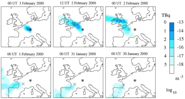
Fig. 1. Normalised retroplumeχˆ1∗(x, t )at ground or sea level corresponding to the 100 mBq.m−3 peak in Freiburg between 02:00 and 10:00 UT on 3 February 2000. In theoryχˆ1∗should be given per kg of air but at ground level it is roughly equivalent and more convenient to give it per m3. The same figure may be read in terms of possible point sourcesq=100 mBq.m−3/χˆ1∗(x, t )with a scale in TBq of133Xe. The circle on the images indicates the position of the detector. The cross describes the backtrajectory of a Lagrangian particle departing back in time from Freiburg on 3 February 2000 at 06:00 UT. Notice that the Lagrangian particle does not follow the centre of the Eulerian retroplume.
A source of intensityQinxatt will generate a measure-mentµ = ˆχ∗(x, t ) Q. In other words a measurement µ can be explained by an instantaneous point source inx att of intensityQ= χˆ∗(µ
x,t ). The retroplume establishes a
con-straint between the position of the source and its intensity. This deterministic character of the quest for macroscopic point sources was simultaneously clarified, during the tech-nical discussions of the Treaty, by Seibert (2000), describing the retroplume as a source-receptor matrix, and Issartel et al. (2000), a conclusion later adopted in the collective report of an ad-hoc expert group (CTBTO/PTS, 2001).
This analysis easily extends to the case of point sources that are not instantaneous. Suppose a source inxhas a rate of releaseQ(t )˙ ≥0 per unit time and a total release isQ= R ˙
Q(t )dt; the measurement isµ=R ˆ
χ∗(x, t )Q(t )dt˙ . AsQ˙ is a non-negative functionµ≤maxtχˆ∗(x, t )RQ(t )dt˙ , or:
Q≥ µ
maxtχˆ∗(x, t )
=Qmin(x) (14)
We still do not know where the source actually lies. It could lie in any position x provided the retroplume went there at some moment. Nevertheless the threshold function
Qmin shows that not all positions are equivalent. A source far away from the detector should be greater than a close one.
The retroplume of the peak measurement of 133Xe in Freiburg has been calculated by model POLAIR according to Eq. 12 with a normalised detector functionπˆ concentrated in Freiburg at positionxF, and during an eight hour interval
1t; the symbol δsp(x)is a Dirac function of the space so that its physical unit is the inverse unit of volume:
ˆ
π (x, t )=
δsp(x−xF)
1t ρ(xF,t ) 2≤t≤10 UT, 2000/02/03
0 otherwise
(15)
Fig. 2. Minimum release from a point source a ground or sea level (a)Qmin(x)compatible with the peak measurement of Freiburg µ1=103 mBq.m−3 (b)Qmin4 (x)compatible with the series of measurements in Freiburgµ0=6,µ1=103,µ2=42,µ3=6 mBq.m−3; this value ofQmin4 (x)would not be altered by considering a fictitious measurement in StockholmµS =0 mBq.m−3on 3 February 2000
(c)Qmin5 (x)compatible with the previous series completed with a fictitious measurementµS=100 mBq.m−3in Stockholm.
Qmincalculated for most western Europe would be compat-ible with a 10 kiloton test.
We have also reproduced the traditional diagnostics of in-vestigating a point source in the neighbourhood of an aver-age current line obtained by integrating back in time from the detector the wind field at or close to the ground level. The curve obtained is generally called a “backtrajectory” or even a “Lagrangian backtrajectory”. We think the method is ill defined for two reasons. Firstly the real backtrajectory of a real particle is a 3D thing that cannot be obtained by just considering the horizontal wind at some given altitude. Sec-ondly, the wind generally dramatically decreases close to the ground so that the result does depend on the altitude chosen for the calculations. As POLAIR is fundamentally a Eule-rian model, we adapted this calculation by just setting verti-cal advection, horizontal and vertiverti-cal diffusions to zero. The tracer was advected back in time by the winds obtained at 32 m above ground or sea level. Because of numerical dif-fusion (Ouahsine and Smaoui, 1999) a little cloud is formed; this effect remains negligible, the horizontal dimension of the cloud after four days (30 January 2000) are about 200 km, four times less than the advection, ten times less than the extension of the retroplume. Hence we reported on Fig. 1 a cross representing the centre of the little cloud as a reali-sation of the traditional diagnostics. This backtrajectory first follows the retroplume but too slowly with the ground winds; on 30 January 2000 the cross is at the edge of the retroplume, thousand kilometres away from its centre. It indicates a pos-sible source in Gascony which is very unlikely as previously commented.
5 Several measurements by a single station
The diagnosis above can be improved so as to determine min-imum total releasesQmin4 (x)taking into account the
con-straints imposed by four measurements obtained in Freiburg. The constraining nature of these additional observations is easy to understand: if the source lies far away, the plume of
133Xe will have much broadened before reaching Freiburg
and it will be detected during a long time. If successive measurements in Freiburg display a narrow peak, the source cannot be too far away. In order to evaluate this effect we handled the following four observations (Arthur et al., 2001) with the peak measurement now labelled 1:
µ0=6 mBq.m−3from 18 to 2 UT, 2000/02/02-03 µ1=103 mBq.m−3from 2 to 10 UT, 2000/02/03
µ2=42 mBq.m−3from 10 to 18 UT, 2000/02/03 µ3=6 mBq.m−3from 18 to 2 UT, 2000/02/03-04
As at ground level one m3 roughly contains one kg of air, we considered the measurements obtained in mBq.m−3to be equivalent to measurements in mBq.kg−1. To each measure-ment a normal retroplumeχˆi∗(x, t )may be related. A source inxwith a rate of releaseQ(t )˙ ≥0 is now subject to the four constraints:
µi =
Z ˆ
χi∗(x, t )Q(t )dt˙ i=0,1,2,3 (16) We considered the following system of constraints were pos-sible errors are taken into account with wide margins (this will be commented in more detail at the end of the section):
˙
Q(t )≥0 0 mBq.m−3≤R
ˆ
χ0∗(x, t )Q(t ) dt˙ ≤10 mBq.m−3 52 mBq.m−3≤R
ˆ
χ1∗(x, t )Q(t ) dt˙ ≤206 mBq.m−3 21 mBq.m−3≤R
ˆ
χ2∗(x, t )Q(t ) dt˙ ≤84 mBq.m−3 0 mBq.m−3≤R
ˆ
˙
Q(t ). This linear optimisation problem can be easily man-aged, when time is discretised, by means of the so called “simplex” algorithm. This classical algorithm was first de-scribed by Dantzig (1963). We operated it locally, with a one hour time step, for each positionxat ground or sea level in western Europe and for sources starting from January the 25th. A well known property of the simplex algorithm is that the optimal rate of release Q˙min(x, t )at position x is non zero for a number of time steps that is at most the number of constraints. The results are reported on Fig. 2b. For most po-sitions the above constraints are not compatible. This means that the 133Xe detected in Freiburg cannot have originated there. The threshold functionQmin4 (x)is clearly more re-strictive thanQmin and the new diagnosis clarifies the pre-vious one. Admissible sources now lie in a narrow strip de-parting from Freiburg to the northwest through France, Bel-gium, Great Britain and terminating one thousand kilometres off Ireland. Industrial sources should not be sought further than Wales. The diagnosis clearly excludes the southern part of France where the previous one already allowed only pro-hibitively big sources. A real advantage is obtained in the western part of France and southern part of England where sources as large as some tenths of kilotons, previously ad-missible, are now excluded.
Notice that a weak source close to Freiburg is not ex-cluded. The four measurements obtained there might have been contaminated by four little releases from a position nearby. And generally when all the measurements will be from a single station, the same number of local contamina-tions will make up an admissible source. Therefore, a single station will never be in a position to exclude a source in its close environment. This difficulty can be partly removed if we assume a limited duration of the release. The duration of industrial releases is classically less than twelve hours, one working day. Such a signal, emitted in the neighbourhood of Freiburg, should not interest more than three eight hour samples. It is nevertheless more convenient to use the local optimisation method with information from several stations. It may be argued that the use of margins in the system of constraints 17 is not compatible with the statistical nature of the measurement errors. In fact the bounds of the margins is determined by our weaker or higher tolerance that the real values of the measurements escape from between them. If we want to be sure that, withp =99% probability, the real measurement lie inside the margins, then we have to use wider margins than would be required forp=90%. Hence the threshold function depends on the prescribed probability:
Qmin4 =Qmin4 (p,x).
6 Measurements from several stations
The local optimisation method described above is just an abridged way to handle the information contained in the
retroplumes. A more accurate understanding of the mete-orological situation may require a complete analysis as we now explain. The event detected on 3 February 2000 was observed only in Freiburg. The CTBT station of Stock-holm was not yet operating. Let’s just imagine what could have been said if a 24 hour sample had been taken there on 3 February 2000. We denote the corresponding normal retroplume asχˆS∗ and the fictitious measurement asµS. A
source inx with a rate of releaseQ(t )˙ would thus lead to µS =RχˆS∗(x, t )Q(t ) dt˙ .
We imagined two situations. Firstly the requirement that
µS = 0 mBq.m−3 has been combined with real data from
Freiburg in the local optimisation. This additional infor-mation would not change the final result. This means that sources previously diagnosed would be mostly compatible with a zero valued measurement in Stockholm in such a way that Fig. 2b is unaltered. Secondly the requirement that
µS = 100 mBq.m−3 would clearly exclude weak sources
close to Freiburg as shown by Fig. 2c. Only big sources northwest of England would be acceptable then.
We now place the transparent figure representing the retro-plumeχˆS∗from Stockholm on top of the figure representing the peak retroplumeχˆ1∗ from Freiburg. Considering the re-sulting Fig. 3 we appreciate the connections of each point in space and time with both measurements. We first notice that the retroplumes intersect marginally. This is the reason why a zero valued measurement in Stockholm does not alter the lo-cal optimisation diagnosis. We still notice that the retroplume from Stockholm does not meet western continental Europe. A source there could not contaminate the sample of Stock-holm and would be excluded by the local optimisation diag-nosis for a virtual measurementµS =100 mBq.m−3. In that
case we notice furthermore that instantaneous spot sources may be considered only in Scotland where the retroplumes intersect marginally. Other acceptable sources should have a duration greater than twelve hours corresponding to the de-lay separating the passings of one and other retroplumes over most positions.
7 Real versus analysed winds: ETEX1
Fig. 3. In blue the normalised retroplumeχˆ1∗associated to the peak detection of 133Xe in Freiburg. In red the normalised retroplume emitted by the virtual measurement sampled in Stockholm between 00:00 and 24:00 UT on 3 February 2000. The retroplumes intersect only marginally in Scotland. The measurements are fundamentally independent. Scotland is in fact the only possible position for an instantaneous point source to contaminate positively both measurements. Both retroplumes flow over Ireland or above the ocean West of Ireland but never simultaneously. A point source there could contaminate both measurements but it could not be an instantaneous source.
from Monterfil, Brittany, France, between 23 October 94, 16:00 UT and 24 October 4:00 UT. Time averaged concentra-tion measurements were delivered each third hour by 168 de-tectors all over Europe. We have selected three stations: F8, Brest, France, west of Monterfil never saw the cloud of pmch and delivered only zero-valued measurements; F20, Reims, France and D10, Essen, Germany were successively on the main way of the cloud. In order to compare the practical achievement of the local optimisation method and the ideal situation of identical forward and backward world we pre-pared a set of synthetic measurements with POLAIR for a source at the prescribed position and time interval. In the following lines the word “practical” will refer to the real sit-uation (forward real world-backward modelled world) and the word “ideal” to the idealised situation (forward modelled world-backward modelled world). We performed a local op-timisation, practically and ideally, with various combinations of F8, F20, D10. The only effect of the zero-valued series of F8 is to exclude possible sources west of Brest.
Because of the difference between the forward real world and the backward modelled world it is necessary to loosen the constraints of the local optimisation. This may be done in two steps in such a way that the practical results finally display a great coherence with the ideal results.
Firstly the model, especially with six hourly meteorolog-ical input data, cannot reproduce with a great accuracy the
3-hourly behaviour of the real cloud, except in the very spe-cial case of F8 not seeing the cloud at all. Then, instead of considering in the simplex algorithm the complete sequence of measurements at F20 or D10, it seems more reasonable to select a few ones to capture the passing of the cloud. We noticed that the ideal results were not significantly different when using complete or partial sequences so that the present strategy may be in fact considered a removal of redundant in-formation. In the case of the Freiburg episode with 8-hourly measurements this removal of redundant information was not necessary.
The strategy, as shown by Fig. 4a, b, d, e enables to ob-tain practical results very coherent with the ideal ones when F20 and D10 are considered separately. If the complete se-quence of measurements at F20 was handled then, as shown in Fig. 4a1, only sources close enough to the station would be compatible. The thresholdQmin = 307 kg diagnosed for Monterfil would not be coherent with the ideal threshold
Qmin = 160 kg. The selection of a few measurements is not so important for D10 probably because the evolution of the signal there has been smoothed on a larger distance to the source. No position at all is jointly compatible with both the sequences of real measurements at F20 and D10, either complete or partial. We still have to loosen the constraints.
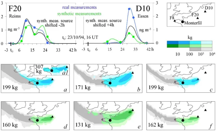
Fig. 4. The upper part of the figure describes the time evolution of the three hourly averaged measurements by stations F20 and D10 after the ETEX-1 release, 340 kg of pmch from Monterfil during 12 hours beginning on 23 October 1994, 16:00 UT : the real measurements (blue curves) and the synthetic measurements simulated by POLAIR (green curves). A better fit is obtained for the synthetic measurements if the twelve-hour release at Monterfil begins at 14:00 UT for F20, at 20:00 UT for D10 (black curves). The coloured dots indicate the measurements selected as sufficient and not excessive constraints for the investigation of possible point sources at ground or sea level. The lower part of the figure shows the result of the simplex algorithm for the stations represented by a triangle with the selected real, on(a)and (b), or synthetic measurements on(d), (e)and(f). When taken into account, the series of zero-valued measurements obtained at F8 just has the effect of excluding otherwise possible sources indicated by grey colours.(a1)is obtained with the simplex algorithm applied to the complete sequence of real measurements by F20.(c)is obtained as a maximin combinationQmaxminof (a) and (b); the blue part of (c) is a maximin combination of the blue parts of (a) and (b). The numbers in kg indicate the minimum amount of tracer diagnosed for a source in Monterfil to be compared to 340 kg.
In the model the travel time of the cloud between two stations is calculated with a shift due to slight errors in the speed of the analysed winds. In the case of ETEX1, a shift more than three hours would break the coherence of real measurements with respect to the calculations so that no simulated source would be compatible with them. It seems this is what hap-pened to F20 and D10; as regards F8, a shift would have no consequence. To see that we shifted in fact the twelve-hour source in Monterfil in order to obtain a better fit of the real and simulated time evolution of the measurements. As shown in the upper part of Fig. 4, the best fit at F20 is ob-tained for a source shifted -2 hours, but for D10 the source should be shifted +4 hours.
A possible strategy is to use the simplex algorithm sepa-rately for F20 and D10 in order to obtain threshold functions
QminF20 andQminD10 and to evaluate a joint threshold constraint asQmaxminF20,D10 = max QminF20, QminD10. Indeed, if Qis the
to-tal amount of tracer released by a point source at positionx, then necessarily:
Q≥QminF20(x) and Q≥QminD10(x)
H⇒Q≥QmaxminF20,D10(x) (18) We called ’maximin’ this strategy which is less constraining than the joint management of all measurements from F20 and D10 in the simplex algorithm. Nevertheless, as visible from Fig. 4c, obtained as a maximin of real measurements, and Fig. 4f obtained as a simplex of the analogous synthetic measurements, the practical diagnostics is very close to the ideal one. Note also that the 199 kg practically diagnosed for Monterfil are consistent with the 340 kg of the real source.
lost. More sophisticated strategies could be proposed to cap-ture such compatibility or incompatibility. In the case of the Freiburg episode, because of the longer sampling intervals, eight hours, we think that no special precaution would be necessary to use the simplex algorithm with several stations, if any. We stress nevertheless that building such figures as Fig. 3 should be considered a pivotal and prudent element of any diagnostics.
Hence, provided some reasonable adaptations are made, the methods described in this paper are robust enough to be handled in an operational context.
8 Conclusions
Among the forty CTBT noble gas stations many are settled in industrial areas close to such civilian sources of133Xe as nu-clear plants or hospitals. On the one hand, it is to be expected that sometimes several stations close to each other will si-multaneously detect abnormal concentrations corresponding to independent local events. On the other hand, nuclear tests are highly unlikely but would most often be seen by several stations as shown by Hourdin and Issartel (2000) for weak explosions of 1 kiloton. The above method enables to dis-criminate between both circumstances. A set of positive data produced by independent local events will hardly be compat-ible with any single point source. For instance, no position is compatible any longer if two zero valued artificial measure-ments are added in Stockholm just before and just after the positive artificial one thus displaying the rapid evolution tied to a local contamination. In an operational situation, after de-termining that a set of measurements corresponds to several sources, it is still possible to investigate various selections of stations in order to determine which ones could have seen a test and which other ones were polluted independently.
This investigation would usefully complement the obser-vation of nuclide ratios that are different for nuclear tests and civilian releases. The discriminating ability of the method proposed here is a real asset with respect to the diplomatic and political aims of the CTBT.
It may be tempting to interpret a set of measurements in terms of an optimal position of the source minimising some quadratic cost function. Besides its increasing complexity if a duration of the source is addressed the method would have two important drawbacks. Firstly, as explained in this paper following the suggestions of Penenko and Baklanov (2001), several positions are often acceptable for the source, the problem is not to define a best one but to determine what is possible. Secondly the best position may fail to be good because a best position is still rashly defined in situations of measurements tied to several independent sources. The reader should wonder which of these is the simplest and most natural question when considering a set of observations: 1) which sources are compatible? 2) which source minimises a quadratic distance to be defined with the observations?
The methods proposed in this paper pertain to a now flour-ishing domain of inverse problems with many new ideas (Ternisien et al., 2000). Many studies are currently published about a number of atmospheric species (van Aardenne et al., 2001; Sportisse and Qu´elo, 2002). These methods gener-ally aim at rebuilding a complex sourceσ (x, t )by means of concentration measurements. The information contained in such measurementsµkmay be summarised into the
follow-ing equations by means of the associated adjoint retroplumes ˆ
χk∗:
µk =
Z
ρ(x, t )χˆk∗(x, t ) σ (x, t ) dxdt (19) This equation or system of equations is linear with respect to the sourceσ and its inversion as such has been proposed by Seibert (2001) in the frame of the CTBT. The system 19 is drastically under-determined. Considering again that the measurement process defines a scalar product we see that measuring theµk amounts to determine the orthogonal
pro-jection of the functionσ (x, t )over the retroplumesχˆk∗(x, t ). The real sourceσcannot be determined exactly but the avail-able information enavail-ables to propose some linear combination of theχˆk∗as an estimation for it. A general theory of such inverse problems, especially the regularisation of the estima-tion by a ’truncated singular value decomposiestima-tion’ (TSVD), has been addressed by Bertero et al. (1985, 1988) in a context dominated by image deblurring purposes.
This is not the approach that has been followed in this pa-per. We did not try to determine a sourceσ, we endeavoured to determine the positionxof a point source. The system 19 is linear with respect toσ (x, t ), not with respect tox. In order to explore which positions x were possible positions for a point source, we have degraded the complete linear sys-tem 19 into local syssys-tems:
µk =
Z ˆ
χk∗(x, t )Q(t ) dt˙ (20)
We used then the linearity of the local systems with respect to a positive local sourceQ(t )˙ to build criteriaQmin(x)or Qminn (x)that are clearly non-linear functions of the position. In the frame of the treaty the calculation of a complex source by linear assimilation techniques would be of interest in order to confirm that a set of positive measurements is due to several local events. An important challenge for this assimilation should be to take into account the non-negative constraint: σ (x, t ) ≥ 0. This theoretic aim has been investigated by de Villiers et al. (1999).
References
Arthur, R. J., Bowyer, T. W., Hayes, J. C., Heimbigner, T. R., McIn-tyre, J. I., Miley, H. S. and Panisko, M. E.: Radionuclide mea-surements for nuclear explosion monitoring, 23rd Seismic Re-search Review: Worldwide Monitoring of Nuclear Explosions, Jackson Hole, Wyoming, 2–5 October 2001.
Baklanov, A.: Modelling of the atmospheric radionuclide transport: local to regional scale, Numerical Mathematics and Mathemat-ical Modelling, INM RAS, Moscow, volume 2, (special issue dedicated to 75-year jubilee of academician G. I. Marchuk), 244– 266, 2000.
Bertero, M., de Mol, C., and Pike, E. R.: Linear inverse problems with discrete data, I: General formulation and singular system analysis, II: Stability and regularisation, Inverse Problems, 1, 301–330, 1985 (part I) and 4, 573–594, 1988 (part II).
Brandt, J., Ebel, A., Elbern, H., Jakobs, H., Memmesheimer, M., Mikkelsen, T., Thykier-Nielsen, S. and Zlatev, Z.: The impor-tance of accurate meteorological input fields and accurate plan-etary boundary layer parameterizations, tested against ETEX-1, in ETEX symposium on long-range atmospheric transport, model verification and emergency response, 13–16 May 1997, Vienna, Austria, Nodop editor, Proceedings, European Commis-sion, EUR 17346 EN, 195–198, 1997.
Carrigan, C. R., Heinle, R. A., Hudson, G. B., Nitao, J. J., and Zucca, J. J.: Trace gas emissions on geological faults as indica-tors of underground nuclear testing, Nature, 382, 528–531, 1996. CTBTO/PTS: Evaluation of the atmospheric transport modelling tools used at the Provisional Technical Secretariat, Report to the PTS of an Ad-hoc Expert Group on the evaluation of atmo-spheric models used at the PTS for radionuclide transport anal-yses, Preparatory Commission for the Comprehensive Nuclear Test Ban Treaty Organization, Vienna, report CTBT/EVA/EG-1/1, 73 pages, 2001.
Dantzig, G. B.: Linear Programming and Extensions, Princeton University Press, 1963.
De Geer, L.-E.: Sniffing out clandestine tests, Nature, 382, 528– 531, 1996.
de Villiers, G. nD., McNally, B., and Pike, E. R.: Positive solutions to linear inverse problems, Inverse Problems, 15, 615–635, 1999. Elbern, H. and Schmidt, H.: A four-dimensional variational chem-istry data assimilation scheme for Eulerian chemchem-istry transport modelling, J.G.R. 104(D15), 1999.
Gallardo, L., Olivares, G., Langner, J., and Aarhus, B.: Coastal lows and sulfur air pollution in central Chile, Atmospheric Envi-ronment, 36, 3829–3841, 2002.
Goyal, P. and Singh, M. P.: The long term concentration of sulphur dioxide at Taj Mahal due to the Mathura refinery, Atmospheric Environment, 24B, 407–411, 1990.
Hourdin, F. and Issartel, J.-P.: Subsurface nuclear tests monitoring through the CTBT xenon network, Geophysical Research Let-ters, 27(15), 2245–2248, 2000.
Issartel, J.-P., Cabrit, B., Idelkadi, A., and Hourdin, F.: Localization of sources for events detected during the noble gas equipment test, in Jean and Seibert editors, Informal Workshop on Meteoro-logical Modelling in Support of CTBT Verification, Vienna, 4–6 December 2000.
Joint Research Centre, Etex. The European tracer experiment, Eu-ropean communities, EUR 18143 EN, ISBN 92-828-5007-2, 107 pp., 1998.
Koren, B.: A robust upwind discretization method for advection, diffusion and source terms, in Vreugdenhil and Koren editors, Numerical methods for advection-diffusion problems, Notes on Numerical Fluid Mechanics 45, 117–138, Braunschweig, Vieweg, 1993.
Kunz, C.: Xe-133: ambient air concentrations in upstate New York, Atmospheric Environment, 23, 1827–1833, 1989.
Lewins, J.: Importance, the Adjoint Function, Pergamon Press, 1965.
Louis, J.-F.: A parametric model of vertical eddy fluxes in the at-mosphere, Boundary Layer Meteorology, 17, 187–202, 1979. Marchuk, G. I.: Sopryazhennye Uravneniya i Analiz Slozhnykh
Sistem, Moskva, Nauka, 1992, translated in English as: Adjoint Equations and Analysis of Complex Systems, Mathematics and its Applications, Hazewinkel (Ed), Kluwer Academic Publisher, 295, 1995.
McCourt, F. R. W., Beenakker, J. J. M., K¨ohler, W. E. and Kuˇsˇcer, I.: Nonequilibrium Phenomena in Polyatomic Gases, Dilute Gases, International Series of Monographs on Chemistry, 18, 1 ,Claren-don Press, Oxford, 1990.
Olivares, G., Gallardo, L., Langner, J., and Aarhus, B.: Regional dispersion of oxidised sulfur in central Chile, Atmospheric Envi-ronment, 36, 3819–3828, 2002.
Ouahsine, A. and Smaoui, H.: Flux-limiter schemes for oceanic tracers: application to the English Channel tidal model, Comput. Methods Appl. Mech. Engrg. 179, 307–325, 1999.
Penenko, V. and Baklanov, A.: Methods of sensitivity theory and inverse modeling for estimation of source term and nu-clear risk/vulnerability areas, Lecture Notes in Computer Science (LNCS), 2074, 57–66, Springer, 2001.
Pudykiewicz, J.: Application of adjoint tracer transport equations for evaluating source parameters, Atmospheric Environment, 32(17), 3039–3050, 1998.
Robertson, L. and Persson, C.: Attempts to apply four dimensional data assimilation of radiological data using the adjoint technique, Radiation Protection Dosimetry, Nuclear Technology Publish-ing, 50, 333–337 1993.
Sartelet, K. N., Boutahar, J., Qu´elo, D., Coll, I., and Sportisse, B.: Development and validation of a 3D chemistry transport model POLAIR3D, by comparison with data from ESQUIF campaign, Proc. of the 6th GLOREAM workshop: Global and regional at-mospheric modelling, Aveiro, Portugal, 4–6 September 2002. Seibert, P.: Methods for source determination in the context of the
CTBT radionuclide monitoring system, in Jean and Seibert ed-itors, Informal Workshop on Meteorological Modelling in Sup-port of CTBT Verification, Vienna, 4–6 December 2000. Seibert, P.: Inverse modelling with a lagrangian particle dispersion
model: application to point releases over limited time intervals, in Gryning and Schiermeier editors, Air Pollution and its Appli-cation XIV, NATO, Kluwer Academic/Plenum Publisher, 381– 389 2001.
Sharan, M., McNider, R. T., Gopalakrishnan, S. G., and Singh, M. P.: Bhopal gas leak: a numerical simulation of episodic disper-sion, Atmospheric Environment, 29, 2051–2059, 1995. Spee, E. J.: Numerical Methods in Global Transport-Chemistry
Models. PhD thesis, Universiteit van Amsterdam, ISBN 90-74795-88-9, 1998.
(RAC-SAM), 96(3), 507–528, 2002.
Sportisse, B. and Qu´elo, D.: Data assimilation and inverse modeling of atmospheric chemistry, to be published in Sharan editor, Spe-cial issue of the Journal of the Indian National Science Academy on Advances in Atmospheric and Oceanic Sciences, 2002. Sweby, P. K.: High resolution schemes using flux limiters for
hyper-bolic conservation laws, SIAM J. Numer. Anal., 21, 995–1011, 1984.
Ternisien, E., Roussel, G., and Benjelloun, M.: Blind localization by subspace method for a scattering model, Proc. Sysid 2000, 2000.
Uliasz, M. and Pielke, R.: Application of the receptor oriented
ap-proach in mesoscale dispersion modeling, in van Dop and Steyn editors, Air Pollution and its Application VIII, NATO, Plenum Publisher, 399–407, 1991.
van Aardenne, J. A., Builtjes, P. J. H., Hordijk, L., Kroeze, C., and Pulles, M. P. J.: Using wind-direction-dependent differences be-tween model calculations and field measurements as indicator for the inaccuracy of emission inventories, Atmospheric Envi-ronment, 36, 1195–1204, 2001.