www.biogeosciences.net/11/5381/2014/ doi:10.5194/bg-11-5381-2014
© Author(s) 2014. CC Attribution 3.0 License.
A mechanistic particle flux model applied to the oceanic
phosphorus cycle
T. DeVries1,2,3, J.-H. Liang1,4,5,6, and C. Deutsch1,7
1Department of Atmospheric and Oceanic Sciences, University of California, Los Angeles, CA, USA 2now at Department of Geography, University of California, Santa Barbara, CA, USA
3also at Earth Research Institute, University of California, Santa Barbara, CA, USA 4Applied Physics Laboratory, University of Washington, Seattle, WA, USA
5now at Department of Oceanography and Coastal Sciences, Louisiana State University, LA, USA 6also at Center for Computation and Technology, Louisiana State University, LA, USA
7School of Oceanography, University of Washington, Seattle, WA, USA Correspondence to: T. DeVries ([email protected])
Received: 3 February 2014 – Published in Biogeosciences Discuss.: 6 March 2014 Revised: 12 July 2014 – Accepted: 26 August 2014 – Published: 7 October 2014
Abstract. The sinking and decomposition of particulate or-ganic matter are critical processes in the ocean’s biological pump, but are poorly understood and crudely represented in biogeochemical models. Here we present a mechanistic par-ticle remineralization and sinking model (PRiSM) that solves the evolution of the particle size distribution with depth. The model can represent a wide range of particle flux profiles, depending on the surface particle size distribution, the re-lationships between particle size, mass and sinking veloc-ity, and the rate of particle mass loss during decomposition. The particle flux model is embedded in a data-constrained ocean circulation and biogeochemical model with a simple P cycle. Surface particle size distributions are derived from satellite remote sensing, and the remaining uncertain param-eters governing particle dynamics are tuned to achieve an optimal fit to the global distribution of phosphate. The res-olution of spatially variable particle sizes has a significant effect on modeled organic matter production rates, increas-ing production in oligotrophic regions and decreasincreas-ing pro-duction in eutrophic regions compared to a model that as-sumes spatially uniform particle sizes and sinking speeds. The mechanistic particle model can reproduce global nutri-ent distributions better than, and sedimnutri-ent trap fluxes as well as, other commonly used empirical formulas. However, these two independent data constraints cannot be simultaneously matched in a closed P budget commonly assumed in ocean models. Through a systematic addition of model processes,
we show that the apparent discrepancy between particle flux and nutrient data can be resolved through P burial, but only if that burial is associated with a slowly decaying component of organic matter such as might be achieved through protection by ballast minerals. Moreover, the model solution that best matches both data sets requires a larger rate of P burial (and compensating inputs) than have been previously estimated. Our results imply a marine P inventory with a residence time of a few thousand years, similar to that of the dynamic N cycle.
1 Introduction
water column, the resupply will occur on faster timescales of seasons to decades, and may follow pathways to lower lat-itudes, where nutrient consumption is complete. Thus, the depths at which particles sink before being remineralized may have a large influence on marine productivity and car-bon pump efficiency (Boyd et al., 2008; Buesseler and Boyd, 2009; Kwon et al., 2010).
The depth scale of decomposition depends on the ratio of the particle sinking velocity and the rate at which the par-ticles are remineralized by bacteria (Sarmiento and Gruber, 2006). For faster sinking speeds or slower remineralization rates, nutrients will be released in deeper waters. However, these two critical rates may themselves be coupled, because particle sinking speeds are strongly influenced by particle size, and particle size is altered by biological rates of decom-position. Given the complexity of these dynamics, and the computational expense of simulating numerous particle size classes, even most sophisticated ecosystem/biogeochemical cycle models still treat particles implicitly, through highly idealized empirical relationships (Martin et al., 1987; Arm-strong et al., 2002). Quantitative and predictive understand-ing of the underlyunderstand-ing biological transformations and their en-vironmental sensitivities remain quite primitive.
We present here a size-resolved model of marine particle dynamics to predict how the particle size spectrum changes as it sinks, depending on the characteristics of surface par-ticles and their alteration by subsurface microbial decompo-sition. The model is based on a general mechanistic equa-tion governing particle dynamics, which has been widely ap-plied in meteorology for precipitating clouds (Hu and Sri-vastava, 1995), and in oceanography for both size-resolved bubble populations (Liang et al., 2013) and sinking particles (Burd and Jackson, 2002; Stemmann et al., 2004a; Kriest and Evans, 1999, 2000; Gehlen et al., 2006). The latter models compare predicted particle fluxes to measurements of par-ticle mass or flux from sediment traps. We take a different approach, and evaluate the particle flux model using clima-tological nutrient distributions, which reflect the long-term spatial patterns and rates of remineralization. We do this by embedding the particle model in a 3-D ocean biogeochem-istry model of the marine phosphorus (P) cycle to investigate the influence of particle sinking and respiration on global nutrient distributions and fluxes. The role of remineraliza-tion depth has been examined in a variety of models before (e.g., Kwon and Primeau, 2006; Kwon et al., 2010; Kriest et al., 2010, 2012). Our study has three advantages. First, it uses a mechanistic formulation of particle dynamics, so that the parameters can be interpreted and validated against lab-oratory and field observations. Second, we use a circulation model whose ventilation rates are constrained by radiocarbon and CFC observations, which allows errors in nutrient fields to be attributed to biases in biogeochemical processes, and not physical ones (Doney et al., 2004; Najjar et al., 2007). Fi-nally, we perform a large number of steady state simulations,
so that the sensitivity and uncertainty can be well character-ized.
2 A size-resolving particle sinking and decomposition model
We begin by presenting a general framework for modeling the flux of particulate organic matter (POM), starting from a population of particles of different sizes falling through the water column. The size distribution,n(unit: number per volume per size increment), of particles with a spectrum of diameters, D, undergoing gravitational settling at size-dependent velocity,ws, and shrinking due to remineraliza-tion at rate dD/dt, evolves over time at a fixed location by:
∂n
∂t = ∇ ·(u+ws)n+ ∂ ∂D
dD dt n
+C+F, (1)
where the terms on the right-hand side represent the diver-gence of the particle flux, particle remineralization, coagu-lation, and fragmentation, respectively. The particle flux is achieved through both fluid velocity, u= [ufvfwf], and the sinking rate,ws, of the particles.
Our focus will be on particle fluxes in the context of the long-term, large-scale general circulation of the ocean inte-rior. Accordingly, we make three simplifications. First, for particles with sinking speeds of order 10 m d−1, the trans-port divergence can be reasonably approximated by the ver-tical particle velocities (i.e.,ws≫wf and horizontal length scales much greater than vertical length scales). Second, we assume that the particle size distribution is in steady state throughout the water column. Finally, we focus on regions below the turbulent boundary layer wherez′(=z−zs) >0,
withzs a nominal mixing depth andzdefined positive
down-wards. Here the fragmentation and coagulation terms are rel-atively small and can be neglected (Boehm and Grant, 2001), although some studies suggest that coagulation can be an im-portant process governing the vertical particle flux below the mixed layer (e.g., Stemmann et al., 2004b). Under these as-sumptions Eq. (1) simplifies to
∂wsn
∂z′ +
∂ ∂D
dD dt n
=0, (2)
which states that the divergence of the flux of particles of a given size is balanced by the conversion of particles from larger size classes to smaller ones. Solutions to this particle equation depend on the sinking rate, the rate of mass loss (i.e., dD/dt), and boundary conditions on the particle size distribution,n, in the surface mixed layer (i.e.,z′≤0).
a power law, which we adopt here:
ws(D)=cwDη, (3)
Sinking rates generally do not increase as quickly with size as do terminal velocities predicted by the Stokes law (i.e.,
η <2). Several other factors also influence sinking speeds,
including the density and shape of particles (McDonnell and Buesseler, 2010). Dead/senescent cells sink much more quickly than living ones, indicating an important role for motility and buoyancy regulation. Resolving all of these fac-tors affecting particle settling speed is beyond the scope of the present study. We assume that variations in these factors are effectively averaged over the scales of interest.
The rate at which particles lose mass involves a complex set of processes by which particles are grazed by filter feed-ers, and colonized by free-living bacteria that hydrolyze or-ganic matter, releasing dissolved oror-ganic matter (DOM) into the surrounding water. We simplify the biological dynamics by assuming that, in each size class, the rate of mass loss is proportional to the particle mass,
dm
dt = −crm, (4)
an assumption that is supported by measurements on phyto-plankton aggregates (e.g., Iversen and Ploug, 2013, Fig. 3). We further assume that the mass of particles increases with size according to
m(D)=cmDζ, (5)
whereζmay be less than 3 to account for the increase in frac-tional water content of larger particle aggregates (Alldredge and Gotschalk, 1988). Combining Eqs. (3)–(5) gives
dD
dt = − cr
ζ D. (6)
An analytic solution to Eq. (2) can be obtained assum-ing that the size distribution of particles in the mixed layer (above z′=0) can be described by a power law (Sheldon et al., 1972; Jackson et al., 1997),
n(z′=0, D)=noD−ǫ, (7)
with no a constant that determines the total mass, and the value ofǫdetermining the size distribution of particles in the well-mixed surface layer. Estimates of surface particle size distribution from satellite observations use the same power-law formulation (Kostadinov et al., 2009), and can therefore be used to incorporate spatially variableǫin a global biogeo-chemical ocean model (see Sect. 3). Under this assumption, a solution to Eq. (2) can be found using the method of char-acteristics,
n(D, z′)=n0D−ǫ
1+ crη
ζ cw
D−ηz′
1−ηǫ
. (8)
(a)
Particle size (m) 100
102
104
106
108
Particle size spectrum (normalized)
10-4 10-3
10-5
Normalized particle flux (mass) 100
10-1
10-2
10-3
Particle flux Particle mass
Particle sinking velocity (m/d)
10 20 30 40 50
4500 4000 3500 3000 2500 2000 1500 1000 500 0
Depth below euphotic zone, z’ (m)
100
101
102
103
104
10-1
10-2
Particle mass (normalized)
0 m 100 m 1000 m 2000 m 4000 m
Particle size (m)
10-4 10-3
10-5
(b)
(c) (d)
Figure 1. (a) The size distribution,n, of particles as a function of
depth and particle size class as predicted by Eq. (8) for the sur-face size rangeDS=20 µm toDL=2000 µm. Black x’s mark the upper size limit of particles at each depth from Eq. (11). (b) The mass of particles within each size class with depth. (c) The nor-malized integrated particle mass and particle flux with depth us-ing the size distribution from (a). (d) The mass-weighted particle sinking velocity with depth. All calculations used the following parameter values:cw=2.2×10⁵m1−ηd−1(Kriest and Oschlies, 2008),ǫ=4.2 (Kostadinov et al., 2009),η=1.17 (Smayda, 1970),
ζ=2.28 (Mullin et al., 1966),cr=0.03 d−1(Kriest and Oschlies, 2008).
According to Eq. (8), the size distribution of particles creases with decreasing particle size, and decreases with in-creasing depth below the mixed layer (Fig. 1a). The total mass of particles can be calculated at any depth by integrat-ing the particle mass,m, and the particle size distribution,n. Near the surface, the bulk of the total particle mass is con-tained in small particles, but this peak shifts towards larger particles deeper in the water column (Fig. 1b). At intermedi-ate depths, the particle mass reaches a maximum at interme-diate sizes (Fig. 1b).
The net conversion of mass from particulate to dissolved forms can be calculated from the mass and flux of particles integrated over the full particle size distribution. The total mass of sinking POM is thus given by
M(z′)= DL(z′)
Z
DS(z′)
n(D, z′)m(D)dD, (9)
and the total sinking flux (mass times velocity) of POM is given by
F (z′)= DL(z′)
Z
DS(z′)
−5000 −4000 −3000 −2000 −1000 0
Depth (m)
ε = 4.2
ζ = 2.28
η = 1.17 c = 0.03r
Normalized particle flux
100
10-1
10-2
10-3
−5000 −4000 −3000 −2000 −1000 0
Depth (m)
Normalized particle flux
100
10-1
10-2
10-3
ε = 5.3
ε = 3.3
ζ = 1.8
ζ = 2.8
η = 1.10
η = 1.25
c = 0.04r
c = 0.02r
(a) (b)
(c) (d)
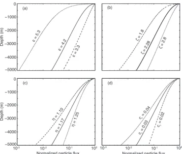
Figure 2. The sensitivity of the normalized particle flux
pre-dicted by the Particle Remineralization and Sinking Model (PRiSM, Eq. 13) to the four parameters controlling the particle flux: (a)ǫ, the exponent in the relationship between particle size and particle size distribution, (b)ζ, the exponent in the relationship between parti-cle mass and partiparti-cle size, (c)η, the exponent in the relationship between particle sinking velocity and particle size, and (d)cr, the degradation rate of sinking particles. Solid curves use the parame-ters from Fig. 1.
whereDS(z′)andDL(z′)are the smallest and largest parti-cle sizes, respectively, which may vary with depth. An upper limit on the size of particles at a particular depth will be set by the size of the largest particles in the euphotic zone. The change in the upper size limit with depth can be evaluated by combining Eqs. (3) and (6) to obtain
DL(z)=max
DL(z′=0)η−c1
η ζz
′
,0 1η
, (11)
where c1=cr/cw. In principle, DS(z′) should vary with depth according to a formula similar to Eq. (11). However, we found very little sensitivity of either the total mass or the total particle flux to a change inDSwith depth, and therefore for simplicity in all our calculations we setDS(z′)=DS(z′= 0). Here and throughout, we assume particle sizes at the sur-face range from DS=20 µm to DL=2000 µm in the eu-photic zone, and use a discretized particle size of dD=2 µm. The total particle mass decreases strongly with depth in the first several hundred meters below the euphotic zone, due to conversion from large to small particles and the loss of particles at the upper end of the size spectrum (Fig. 1c). The total particle mass decreases approximately log-linearly with depth below about 1000 m below the euphotic zone as the mass spectrum becomes flatter (Fig. 1b). The total particle flux is heavily weighted toward the sinking flux of the largest
(heaviest) and fastest-sinking particles, and therefore is not as strongly attenuated with depth as the total mass flux (Fig. 1d). The average (mass-weighted) particle sinking velocity is defined as,
ws(z′)=
F (z′)
M(z′). (12)
For the particular combination of parameters in Fig. 1,ws in-creases with depth up to about 2500 m below the euphotic zone, due to the shift in the mass spectrum toward larger particle sizes at depth (Fig. 1b and d). The average parti-cle sinking velocity then begins to decrease with depth be-low 2500 m as the largest particles begin to disappear com-pletely, resulting in a decrease in the upper particle size limit (see Eq. 11 and Fig. 1a) and an overall shift toward smaller and slower sinking particles (Fig. 1d). An increase in particle sinking velocity with depth is consistent with some observa-tions (Berelson, 2002; McDonnell and Buesseler, 2010) and is implicit in the widely used power-law used to describe the attenuation of particle flux with depth (Martin et al., 1987; Kriest and Oschlies, 2008). Here we see that the particle sink-ing speed can decrease with depth in the abyssal ocean if large particles begin to degrade fully. The protection of sink-ing POM by ballast mineral assemblages (e.g., Armstrong et al., 2002) could counter this deep trend by ensuring a sup-ply of large particles to the deep ocean and thus a contin-ued increase in the average particle sinking speed with depth. This possibility is addressed in Sect. 4.3.
The decrease in POM flux with depth depends on several parameters, which can be seen by rewriting Eq. (10) in the form
F (z′)=cF
DL(z′)
Z
DS
Dζ+η−ǫ
1+c1
η
ζD
−ηz′
1−ηǫ
dD, (13)
wherecF=nocmcw. The actual value ofcFis arbitrary, and in practice we always setcF=1/F (z′=0)so that Eq. (13) is normalized by the flux at the base of the euphotic zone. Thus, there are four parameters that control the particle flux profile:
ζ,η,ǫandc1. We varied these parameters within plausible ranges to examine the sensitivity of the particle flux profile (Fig. 2).
The POM fluxes,F (z′), show similar sensitivities toǫ, the exponent of the surface particle size distribution, andζ, the exponent in the relationship between mass and particle size (Fig. 2a and b). Both an increase inǫ and a decrease in ζ
have the effect of shifting the particle mass spectrum toward smaller masses, which results in more POM being respired near the surface and less POM reaching the deep ocean.
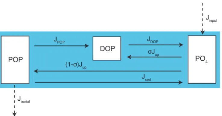
POP
DOP
PO4
(1-σ)Jup
σJup JDOP JPOP
Jsed
Jburial
Jinput
Figure 3. Schematic illustrating the transformations between the
various phosphorus pools in the model: particulate organic phos-phorus (POP), dissolved organic phosphos-phorus (DOP) and inorganic phosphate (PO4). The JPOP term is parameterized according to PRiSM as described in Sects. 2 and 3.
effects onF (z′). Increasingηresults in faster-sinking parti-cles that penetrate deeper into the ocean, while reducing the degradation rate cr has a similar effect on the particle flux profile (Fig. 2c and d). Within this parameter space, the slope of the surface particle size distribution has the largest effect on POM flux to the deep ocean. We will therefore pay partic-ular attention to the influence of variations in this parameter on the large-scale nutrient fluxes in the global biogeochemi-cal model that follows.
3 Phosphorus cycle simulations in a global ocean model The global and long-term distribution of nutrients such as PO4 provides a strong constraint on the patterns and rates of remineralization implied by particle flux models. To ex-ploit the information in these observations, and to derive ap-propriate parameters for the particle sinking model, we in-corporate it into a global ocean circulation/biogeochemistry model. This can be done by simply using the normalized par-ticle flux profiles Eq. (13) at each grid point, which we re-fer to as the Particle Remineralization and Sinking Model (PRiSM). In PRiSM, all the essential dynamics of a size-resolved particle spectrum are included without the compu-tational expense of explicitly simulating that spectrum. 3.1 Model formulation
We model the internal cycling of phosphorus (P) in the ocean as it is transformed between the particulate organic phospho-rus (POP), dissolved organic phosphophospho-rus (DOP) and inor-ganic phosphate (PO4) pools (Fig. 3). Only DOP and PO4 are explicitly carried as tracers in the model – the effects of POP formation and degradation are treated implicitly as de-scribed below. The governing equations for PO4 and DOP
cycling are dPO4
dt = APO4−Jup+JDOP (14)
+ Jsed−Jburial+Jinput,
dDOP
dt = ADOP−JDOP+σ Jup+JPOP, (15)
where A is a matrix transport operator that represents the combined effects of advection and eddy diffusion, and is de-rived from a data-constrained ocean circulation model (De-Vries and Primeau, 2011; De(De-Vries et al., 2012; De(De-Vries, 2014). The uptake of PO4 to form organic matter (Jup) is parameterized by restoring to observed phosphate (PO4,obs) in the euphotic zone (taken to be the same as the mixing depth,zs) wherever modeled PO4exceeds observed PO4 us-ing a restorus-ing timescale ofτb=30 days (Najjar et al., 2007),
Jup=max
1
τb
PO4−PO4,obs
,0
, z′≥0. (16)
The model circulation is steady state, and does not resolve the seasonal cycle, and so we interpolate the 2009 World Ocean Atlas annual mean objectively mapped PO4 concen-trations (Garcia et al., 2010) to the model grid to obtain PO4,obs. A fractionσ of the production is routed directly to DOP in the euphotic zone, and the remainder is routed to POP (Fig. 3). DOP is respired to PO4in a first-order reaction with decay rateκ,
JDOP=κDOP. (17)
The cycling of POP is treated implicitly in the model. The rate of POP export at the base of the euphotic zone is
Feu=(1−σ )
0 Z
zs
Jupdz, (18)
and below the euphotic zone POP is assumed to degrade in-stantaneously to DOP with a vertical distribution dictated by the particle flux profile,
JPOP= ∂
∂z Feu×F (z
′
). (19)
The remaining terms in Eqs. (14) and (15) represent the P budget of the ocean as a whole. TermJsed represents the
source of PO4in the bottom box due to the flux of POP that hits the sea floor and is regenerated. In general, we allow a fraction (fB) of that benthic flux to be buried permanently, so that
Jsed= 1
1zFR(1−fB) (20)
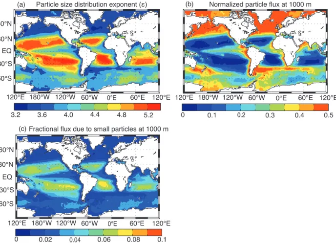
Particle size distribution exponent (ε)
3.2 3.6 4.0 4.4 4.8 5.2
120°E 60°E
0°E 60°W 120°W 180°W
120°E 60°S 30°S EQ 30°N 60°N
(a) (b) Normalized particle flux at 1000 m
120°E 60°E 0°E
60°W 120°W 180°W 120°E
60°S 30°S EQ 30°N 60°N
0 0.1 0.2 0.3 0.4 0.5
120°E 60°E
0°E 60°W 120°W 180°W 120°E
0 0.02 0.04 0.06 0.08 0.1
Fractional flux due to small particles at 1000 m (c)
Figure 4. (a) Spatial variability in the exponent for the surface particle size distribution used in PRiSM. Lower values ofǫindicate larger
particles, and higher values ofǫindicate smaller particles. (b) Spatial variability in the particle flux at 1000 m depth resulting from variability in the surface particle size distribution. (c) The fraction of the flux at 1000 m due to small particles (less than 200 µm in diameter). For (b) and (c) we used the same parameters of PRiSM as in Fig. 1.
cell. Similarly, the rate of total P loss due to burial can be computed from
Jburial= 1
1zfBFR. (21)
At steady state, the rate of P burial in the sediments is matched by allochthonous inputs of P to the ocean, soJinput
is required to satisfy Z
V
JinputdV = Z
V
JburialdV =Ri. (22)
Ri must be specified in order to obtain a solution to
Eqs. (14)–(15). The allochthonous P inputs could include dis-solved and particulate P in river runoff, aeolian deposition of P in atmospheric dust, and terrestrial P from ice-rafted de-bris (Wallman, 2010). For simplicity, and because the spa-tial distribution and magnitudes of allochthonous P inputs are poorly constrained, we assume a uniform rate of P input over the entire model ocean surface. The terms in Eqs. (14)–(15) involving the remineralization (Jsed) and burial (Jburial) of
organic matter in the sediments, as well as the allochthonous inputs of PO4(Jinput), are treated differently in various dif-ferent model configurations, as described in the upcoming Sects. 4.1–4.3.
Equations (14–22) together with Eq. (13) constitute a com-plete model of the P cycle built upon a size-resolved model of particle sinking and remineralization. To calculateF (z′)
we must specify the parameters of PRiSM (Eq. 13), which is described in the next section.
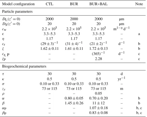
3.2 Model validation and parameter estimation
Table 1. Parameters of PRiSM (Eq. 13) and the biogeochemical models used to simulate the oceanic P cycle: CTL (control simulation
without P burial or allochthonous P inputs), BUR (with P burial and allochthonous P inputs), and BUR+BAL (as BUR, but including effects of ballast-protected sinking particles).
Model configuration CTL BUR BUR+BAL Note
Particle parameters
DL(z′=0) 2000 2000 2000 µm
DS(z′=0) 20 20 20 µm
cw 2.2×10⁵ 2.2×10⁵ 2.2×10⁵ m1−ηd−1
ǫ 3.3–5.3 3.3–5.3 3.3–5.3 – a
η 1.17 1.17 1.17 –
cr (29±3)−1 (31±4)−1 (21±2)−1 d−1 b
ζ 1.62±0.11 1.61±0.11 1.72±0.13 – b
cr, P – – (365)−1 d−1 c
ζP – – 2.28 – c
Biogeochemical parameters
τ 30 30 30 d
κ 0.5 0.5 0.5 yr−1
σ 0.10 or 0.33 0.10 or 0.33 0.10 or 0.33 –
zs 73 or 115 73 or 115 73 or 115 m
ρ – – 0.05 –
α – 0.80±0.05 0.70±0.20 – b
β – 1.45±0.26 11±12 – b
αP – – 1.07±0.18 – b, c
βP – – 0.83±0.08 – b, c
aFrom satellite-based estimates by Kostadinov et al. (2009).bDetermined from optimal fit of the model to PO 4
observations.cFor ballast-protected POP.
smaller particles are more abundant (Fig. 4a). As expected from the PRiSM particle flux profiles (Fig. 2), this results in large spatial variability in the fraction of POM reaching the deep ocean. The normalized particle flux at 1000 m be-low the euphotic zone varies approximately tenfold, ranging from about 0.5 in regions of large particles (ǫ.3.5) to less than 0.05 in regions of very small particles (ǫ&5) (Fig. 4b). Most of the particle flux reaching the deep ocean is due to the sinking of large particles. Small particles less than 200 µm in diameter contribute less than 10 % of the total particle flux at 1000 m depth (Fig. 4c). Away from the sub-tropical gyre re-gions, small particles generally contribute less than 5 %, and as little as 1 %, to the total particle flux at 1000 m (Fig. 4c). The spatial patterns shown in Fig. 4b and c are robust to vari-ations in the values of the parameters controlling the particle flux profile.
The values of the other parameters controlling the particle flux profile,η,ζ, andcr, may also vary spatially due to vari-ability in ecosystem structure and bacterial abundance. How-ever, lacking specific information about their spatial variabil-ity, and for simplicvariabil-ity, we adopt spatially uniform values of these parameters here. Ideally, we would like to determine values for all of these parameters by adjusting them to obtain an optimal fit of the modeled PO4distribution to the observed PO4distribution. However,η(the exponent in the
relation-ship between particle size and sinking velocity) andcr (the degradation rate of POM) have nearly identical influences on the shape of the particle flux profile (Fig. 2c and d). For this reason, we fix the value ofηat 1.17, as determined from ob-servations (Smayda, 1970), and determineζ andcr through an optimization procedure.
The “optimal” model is determined by minimizing the volume-weighted misfit between modeled and observed PO4 concentrations,
f =
Z
V
(PO4−PO4,obs)2dV , (23)
with different euphotic zone depths (73 m or 115 m, corre-sponding to the base of the second and third model layers, respectively). For each given set of fixed parameters,O(102) model simulations are needed to find the optimal set of con-trol parameters. This large number of model simulations is made possible by applying a Newton–Krylov method to find the equilibrium solution to the governing Eqs. (14)–(15).
To focus more clearly on the effects of sinking particles on the vertical PO4 distribution, we also investigated dis-tributions of “regenerated” PO4, which is phosphate that is derived from remineralized organic matter, rather than the “preformed” PO4that is transported conservatively into the deep ocean from regions of incomplete surface utilization. We estimate preformed phosphate (pPO4) by solving for the equilibrium distribution of PO4subject to the condition that all PO4in the euphotic zone is preformed, and there are no interior sources or sinks. Regenerated phosphate (rPO4) is then computed from
PO4=pPO4+rPO4. (24)
Preformed PO4 is calculated from observed and modeled PO4 distributions in the same way, using using either ob-served surface PO4or the PO4simulated by the model, re-spectively. The concentration ofrPO4implied by the obser-vations depends on the depth of the euphotic zone used in the calculation, which is either 73 m or 115 m. This gener-ates a range of “observed”rPO4that we use as an uncertainty estimate.
As a further check on the appropriateness of the model solution, we compare model-derived particle flux profiles to observations of particle fluxes from equatorial Pacific sedi-ment traps (Berelson, 2001). Sedisedi-ment trap data are not in-cluded as a quantitative constraint on the model solution due to the large degree of scatter in the particle trap data (cf. Gehlen et al., 2006, Fig. 3) and the lack of ancillary data (e.g., surface particle size distributions) needed for a direct model/data comparison. It is also difficult to weigh the rel-ative strengths of the PO4and sediment trap data appropri-ately as constraints on model parameters. However, we find that the equatorial Pacific sediment traps provide a valuable qualitative check on the model solution that helps to identify significant biases in the modeled deep-ocean particle flux. This is discussed in more detail in Sect. 4.
4 Results
Here we discuss the results from a hierarchy of model con-figurations designed to evaluate the ability of PRiSM to re-produce the time-averaged distribution of PO4. We focus in particular on depth profiles of PO4and regenerated PO4, as these are very sensitive to the particle flux profile.
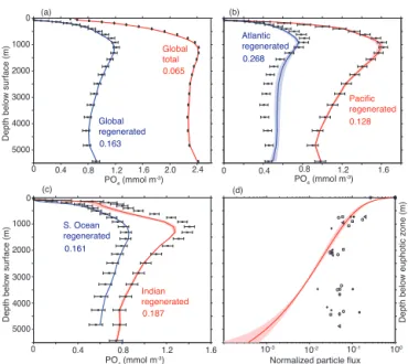
5000 4000 3000 2000 1000 0
0.065
0.134
10-2 10-1
10-3 100
(a) (b)
(c)
Normalized particle flux
PO4 (mmol m
-3)
0 0.4 0.8 1.2 1.6 2.0 2.4 0 0.4 0.8 1.2 1.6
Depth below surface (m)
0.167
0.276
0.184
0.164
PO4 (mmol m
-3)
Pacific regenerated
Atlantic regenerated
Global total
Global regenerated
Indian regenerated
S. Ocean regenerated
5000 4000 3000 2000 1000 0
Depth below surface (m)
0.4 0.8 1.2 1.6
0
PO4 (mmol m
-3)
Depth below euphotic zone (m)
(d)
Figure 5. (a) Globally averaged depth profile of total PO4 (red
curve) and regenerated PO4(rPO4, blue curve), for the CTL model and the observations (blackx+error bars). (b) Modeled (curves
plus shading indicating uncertainty) and observed (blackx+error
bars) rPO4 averaged over the Pacific (red) and Atlantic (blue) oceans. (c) Same as (b) for the Indian (red) and Southern (blue) oceans. (d) Modeled particle flux profile (red curve plus shading in-dicating uncertainty) forǫ=4.2, and observed particle fluxes from sediments traps in the equatorial Pacific (symbols). Printed on (a–
c) is the normalized root mean squared error (RMSE divided by
the average PO4orrPO4concentration) for the CTL model for the region and data type displayed.
4.1 Control simulation
In the control simulation (CTL), we ignore the effects of or-ganic matter burial. In this case, any POP that reaches the sediments is instantaneously remineralized there (i.e.,fb= 0). In these simulations, theJburial andJinput terms are
re-tained, but are so small that they do not affect the distribution of PO4or DOP, and simply serve to set the modeled total PO4 inventory to the observed value. This is accomplished by set-ting theJburial term to remove PO4everywhere in the ocean at a rate ofrg= 10−6yr−1, while theJinput term everywhere restores modeled PO4to the observed mean PO4at the same rate (cf. Primeau et al., 2013; Holzer et al., 2014).
Kriest and Oschlies (2013) had a normalized RMSE of 0.10 for PO4. The model displays a very good fit to the “ob-served” globally averaged vertical profile ofrPO4(Fig. 5a). The model performs worst in the lower mesopelagic zone (∼500–1500 m depth), where modeledrPO4concentrations are slightly lower than observed. Since the model circula-tion is constrained to match radiocarbon and CFC-11 ob-servations (cf. DeVries and Primeau, 2011; DeVries et al., 2012), the lower-than-observed rPO4 in this region proba-bly indicates too little organic matter remineralization there. The model also predicts slightly higher than observed abyssal rPO4concentrations (below∼3000 m depth), suggesting too much deep ocean remineralization. The deficiencies in the modeled vertical distribution of rPO4 can be seen more clearly on the basin scale (Fig. 5b and c). The slightly too high abyssalrPO4concentrations in the model are primarily in the deep Atlantic Ocean (Fig. 5b). Too low mesopelagic
rPO4concentrations can be traced to the Indian Ocean in the depth range 200–2000 m (Fig. 5c).
Given the overall excellent fit of the model to observed PO4andrPO4, and particularly their vertical distributions, one might expect that the model also produces a good fit to independent observations of POM settling from suspended sediment traps. However, this is not the case. In the CTL model, the optimal values of the parameters (Table 1) pro-duces a particle sinking profile that rapidly deflects to very low values in the deep ocean (Fig. 5c). By contrast, obser-vations from sediment traps in the equatorial Pacific Ocean (Berelson, 2001) suggest that the particle flux remains fairly constant below about 2000 m below the euphotic zone, at between 1 and 10 % of the flux at the base of the euphotic zone (Fig. 5c). Sediment traps from other locations such as the Arabian Sea, the North Atlantic, and the Southern Ocean show similar normalized particle flux values in the deep ocean (Berelson, 2001).
Thus, in the CTL model there is a conflict between the ver-tical attenuation of the particle flux implied by the observed PO4distribution, and that measured by sediment traps. The conflict is particularly severe in the deep ocean (Fig. 5c). It arises because for the model to match deep ocean PO4 values, it must assign a fast rate of remineralization, to pre-vent a large particle flux into the deep ocean. This tendency is not unique to this model. In nearly every model used in Phase 2 of the Ocean Carbon Cycle Model Intercomparison Project (OCMIP-2), PO4 concentrations in the deep ocean were significantly overestimated (Najjar et al., 2007, Fig. 8). All of these models used a power-law depth dependence of the sinking POP flux, the so-called “Martin curve” (Martin et al., 1987), and assumed a closed P budget. Since the Mar-tin curve was derived from particle flux profiles from sedi-ment traps, models using the Martin curve naturally overes-timate remineralization in the deep ocean if burial of POM is not allowed (Kriest and Oschlies, 2013). Given the long residence times of abyssal waters, small errors in deep-ocean
5000 4000 3000 2000 1000 0
0.065
0.128
10-2 10-1
10-3 100
(a) (b)
(c)
Normalized particle flux
PO4 (mmol m
-3)
0 0.4 0.8 1.2 1.6 2.0 2.4 0 0.4 0.8 1.2 1.6
Depth below surface (m) 0.163
0.268
0.187
0.161
PO4 (mmol m
-3)
Pacific regenerated
Atlantic regenerated
Global total
Global regenerated
Indian regenerated
S. Ocean regenerated
5000 4000 3000 2000 1000 0
Depth below surface (m)
0.4 0.8 1.2 1.6
0
PO4 (mmol m
-3)
Depth below euphotic zone (m)
(d)
Figure 6. As Fig. 5, but for the BUR model.
POM remineralization rates may accumulate into large bi-ases in PO4.
One obvious solution to these biases is to allow part of the benthic particle flux to be buried permanently, rather than remineralized to PO4 at the sea floor. This solution was examined by Kriest and Oschlies (2013), who found that explicitly modeling organic P burial was necessary in order to achieve a good fit to benthic PO4 concentrations in a model that used the Martin curve parameterization for sinking POM. However, biases in circulation could also con-tribute to the deep-ocean PO4bias. In the following sections we explore whether adding organic matter burial can resolve the conflict between the particle flux attenuation implied by PO4 observations and that derived from sediment traps, in a data-constrained circulation model.
4.2 Including the effects of organic matter burial We now consider a model (BUR) in which we include the burial of POP in the sediments. We assume that the fraction of POP that is buried in sediments,fB, can be related to the “rain rate” at which POP is delivered to the sea floor, FR, following the relationship
fB=tanh(αFβ
−1
R ). (25)
Equation (25) is similar to the relationship used by Burdige (2007) and Kriest and Oschlies (2013), except that here we apply the tanh function to the right-hand side to ensure that the burial efficiencyfBdoes not exceed 1.
We jointly optimized the parameterscrandζ, along with the new parametersα,β, andRi(the rate of allochthonous P
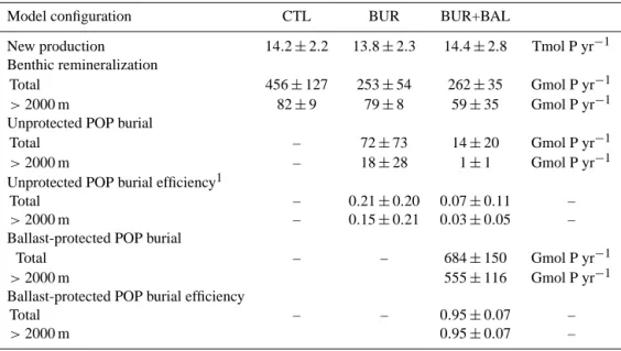
Table 2. Rate of P production, benthic remineralization, and burial from the three different P cycle models considered here.
Model configuration CTL BUR BUR+BAL
New production 14.2±2.2 13.8±2.3 14.4±2.8 Tmol P yr−1 Benthic remineralization
Total 456±127 253±54 262±35 Gmol P yr−1
>2000 m 82±9 79±8 59±35 Gmol P yr−1
Unprotected POP burial
Total – 72±73 14±20 Gmol P yr−1
>2000 m – 18±28 1±1 Gmol P yr−1
Unprotected POP burial efficiency1
Total – 0.21±0.20 0.07±0.11 –
>2000 m – 0.15±0.21 0.03±0.05 –
Ballast-protected POP burial
Total – – 684±150 Gmol P yr−1
>2000 m 555±116 Gmol P yr−1
Ballast-protected POP burial efficiency
Total – – 0.95±0.07 –
>2000 m 0.95±0.07 –
1Burial divided by (burial + benthic remineralization).
andζ, are very similar for the BUR and CTL models (Ta-ble 1). The optimal values ofαandβare about 0.8 and 1.45, respectively (Table 1). The optimal rate of allochthonous P inputs is about 70 Gmol P yr−1, and about 20 % of organic matter reaching the sediments is buried there, although the uncertainty on these quantities is about 100 % (Table 2).
Overall there is very little difference between the PO4 dis-tribution in the BUR and CTL models (compare Figs. 6 and 5). There is a slight improvement over most ocean basins in the fit of the model to the observed rPO4 (Fig. 6b and c). The particle flux profiles in the BUR and CTL models are also very similar (Fig. 6d and Fig. 5d). The misfit between the particle flux predicted by the model and that observed from sediment traps in the deep ocean is still very evident (Fig. 6d). Thus, we conclude that the addition of organic mat-ter burial by itself is not sufficient to resolve the conflict be-tween the particle flux attenuation implied by the PO4 obser-vations, and that implied by the sediment trap observations.
The reason that burial alone cannot reconcile the nutrient distributions with sediment trap data is that the burial rate is proportional to the benthic flux of POM, and thus decreases rapidly with depth. Burial of P in deep sediments permits a larger particle flux to reach the deep ocean without creating a surplus of PO4. However, because of the rapid particle flux attenuation, this would require even more P removal from shallower depths, creating a low PO4 bias there. To fit the PO4globally, the model therefore must maintain a low rate of PO4burial overall. This trade-off between PO4biases in the deep and mid-depth water column would be less stringent if the flux of POM did not decrease so rapidly with depth. This suggests that one solution to the apparent discrepancy between the particle flux data and the PO4distribution is for
a fraction of the sinking flux of particulate P to be relatively recalcitrant. This would allow its flux to decrease less rapidly downward, so that burial from the deep sea could be achieved without slowing PO4 regeneration too much in the thermo-cline. The need for a component of POM that resists degra-dation has been proposed as an explanation for the constancy of the deep particle fluxes, with protection of organic mat-ter from bacmat-terial degradation by inclusion in ballast mineral assemblages as a specific mechanism for it (e.g., Armstrong et al., 2002; Francois et al., 2002; Klaas and Archer, 2002). We test this hypothesis in the model as described in the next section.
4.3 Including the effects of ballast-protected organic matter
Here we separate the flux of sinking POM into two pools with different time scales of degradation to investigate the effects of a slowly degrading P pool on the total particle fluxes and PO4 distributions. As a basis for this separation, we adopt the hypothesis that mineral ballast acts to protect some organic matter from bacterial degradation (Armstrong et al., 2002; Francois et al., 2002; Klaas and Archer, 2002). Other mechanisms for creating a more slowly degraded com-ponent of particulate P are also possible, however. In par-ticular, the recent discovery of significant concentrations of polyphosphates in organic matter in both the water column and sediments (Diaz et al., 2008) will be discussed below as an alternative interpretation of the model results.
2006). This mechanism was explored in the model of Gehlen et al. (2006), who found that the combined effects of particle aggregation and mineral ballasting resulted in large particle fluxes to the deep sea. Here we do not explicitly simulate scavenging of ballast minerals onto sinking organic matter particles, but make the simplifying assumption that the frac-tion of POM that is ballast protected is proporfrac-tional to the flux of ballast minerals out of the euphotic zone (Armstrong et al., 2002). In this case we can express the total flux of POP as the sum of an unprotected component and a ballast-protected component,
F (z′)=(1−fP)FU(z′)+fPFP(z′), (26)
wherefPis the fraction of the POP produced in the euphotic zone that is routed to the ballast-protected POP pool,FU(z′) is the particle flux profile for unprotected POP, andFP(z′)is the particle flux profile for ballast-protected POP. We assume that fP is proportional to the “ballast ratio”,RB, which is the mass ratio of the sinking flux of ballast minerals to the sinking flux of organic carbon at the base of the euphotic zone,
fP=ρRB. (27)
Our P cycle model does not simulate ballast mineral or organic carbon fluxes, and so we use values of RB from the Geophysical Fluid Dynamics Laboratory Earth System Model (GFDL-ESM) to calculate fP (see Appendix A and Fig. A1). Following Armstrong et al. (2002), the value ofρ
is assumed to be 0.05. With these values forρ andRB, the value offPvaries between 0.04 and 0.25, with a mean value of 0.11.
We model the sinking of unprotected and protected POP separately. For protected POP, we use the same parameters as for unprotected POP, except that rather than solving for
cr andζ as part of the inversion, we fix these parameters at values that give reasonable ballast mineral flux profiles. According to Armstrong et al. (2002),FP≈0.4 in the deep ocean. Assumingζ =2.28 (Mullin et al., 1966), and for an averageǫvalue of 4.2, a value ofcr=(365 d)−1gives a value ofFP=0.4 at about 5000 m below the base of the euphotic zone. These then are the parameter values we specify for sinking POP that is ballast protected (Table 1). Because the protected POP is protected from bacterial degradation, we expect it to be buried with a much greater efficiency. There-fore, we use different values ofαandβ in Eq. (25) for pro-tected and unpropro-tected POP.
The resulting model that includes both organic matter burial and ballast mineral effects (BUR+BAL) has seven un-known parameters:cr,ζ,α,β,Ri, andαP andβP (for pro-tected POP). We jointly optimized these parameters using the same procedure as for the CTL and BUR models. The opti-mal value ofcris about(21 d)−1, lower than the∼(30 d)−1 in the CTL and BUR models (Table 1). This degradation rate for unprotected POP is nearly 20 times faster than that
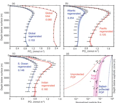
5000 4000 3000 2000 1000 0
0.060
0.125
10-2 10-1
10-3 100
(a) (b)
(c)
Normalized particle flux PO4 (mmol m
-3)
0 0.4 0.8 1.2 1.6 2.0 2.4 0 0.4 0.8 1.2 1.6
Depth below surface (m) 0.153
0.254
0.160
0.146
PO4 (mmol m -3)
Pacific regenerated
Atlantic regenerated
Global total
Global regenerated
Indian regenerated
S. Ocean regenerated
5000 4000 3000 2000 1000 0
Depth below surface (m)
0.4 0.8 1.2 1.6
0
PO4 (mmol m -3)
Depth below euphotic zone (m)
(d)
Unprotected POP
Ballast-protected POP Total POP
Figure 7. As Fig. 5, but for BUR + BAL model. In (d), the average
sinking fluxes of unprotected POP (dashed red curve) and ballast-protected POP (dashed blue curve) are shown separately. The un-certainty on the total POP sinking flux (magenta curve + shading) reflects uncertainty on the parameterscrandζof PRiSM, and spa-tial variability in the ratio of ballast mineral to organic carbon flux at the base of the euphotic zone (see Fig. A1).
assumed for ballast-protected POP. On average, 95 % of ballast-protected POP reaching the sediments is buried there, while only 7 % of unprotected POP reaching the sediments is buried (Table 2). The absolute rates are discussed in the next section.
5 Discussion
The magnitude of organic P production is relatively constant among the model configurations (Table 2). Total organic P production ranges from 13.8±2.3 Tmol P yr−1in the BUR model to 14.4±2.8 Tmol P yr−1 in the BUR+BAL model (Table 2). For comparison, Dunne et al. (2007) used satellite chlorophyll observations and empirical models to estimate that 9.6±3.6 Pg C yr−1is exported out of the euphotic zone as particles. Assuming a C : P ratio of 106:1 in fresh organic matter (Anderson, 1995) and that 80 % of organic matter pro-duction is exported as sinking particles (Hansell et al., 1997), yields a rate of organic P production of 9.4±3.5 Tmol P yr−1. This is on average smaller than the rate of P production de-rived here, but the estimates agree within their relatively large uncertainties.
In contrast to total POM production, the model configura-tions yield substantial differences in the latitudinal patterns of P fluxes within the ocean, and in the total input/output budget of P. These are discussed in the next two sections. 5.1 Implications for P cycling
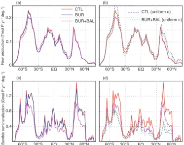
Here we consider the influence of two characteristics of the surface particle distribution – the surface particle size dis-tribution and the ballast ratio – on the internal cycling of P. We find that both of these effects lead to a reduction in the latitudinal variation of export and subsequent deep reminer-alization.
The largest difference in organic P production among the model configurations is caused by the inclusion of ballast-mineral protection in the model BUR+BAL. Relative to the models without ballast-mineral protection, production is re-duced in the Southern Ocean and increased in the tropical and sub-tropical oceans (Fig. 8a). This is due to the effect of ballast minerals on the remineralization profile of sink-ing organic matter. In the Southern Ocean, the ballast ratio is relatively high due to high production rates of biogenic sil-ica associated with diatom-dominated communities. Because the ballast ratio is high, particles sink deeper on average be-fore remineralizing, and therebe-fore the supply of remineral-ized nutrients to surface waters, which can fuel new produc-tion, is reduced. The opposite effect occurs in the tropical and sub-tropical ocean, where the ballast ratio is low (Appendix Fig. A1).
The surface particle size distribution may also have a sig-nificant effect on organic matter production. To evaluate this, we re-ran each of the models in the CTL and BUR + BAL configurations using a spatially uniform surface particle size distribution, with ǫ=4.2, in place of the spatially variable
ǫ used in the standard configuration (see Fig. 4). The re-sults show a significant effect of the particle size distribu-tion on organic matter producdistribu-tion rates. With a spatially vari-able surface particle size distribution, organic P production rates are reduced in regions of high productivity, and
en-New production (Tmol P
yr
-1 deg. -1)
0 0.1 0.2
60°S 30°S EQ 30°N 60°N
CTL BUR BUR+BAL
(a) (b)
BUR+BAL (uniform ε)
60°S 30°S EQ 30°N 60°N
Benthic remineralization (Gmol P
yr
-1 deg. -1)
60°S 30°S EQ 30°N 60°N 60°S 30°S EQ 30°N 60°N
(c) (d)
0.4 0.8 1.2
CTL (uniform ε)
Figure 8. (a) New production by latitude for the CTL, BUR, and
BUR+BAL models (averaged over the four different model config-urations). (b) As (a), but comparing new production rates for the CTL and BUR+BAL models using the standard spatially varying
ǫvalues, and a spatially uniform value ofǫ=4.2. (c) As (a), but showing benthic remineralization below 2000 m. (d) As (b), but for benthic remineralization below 2000 m.
hanced in regions of low productivity in both the CTL and BUR+BAL models (Fig. 8b). This effect occurs because re-gions of high productivity tend to be dominated by larger particle assemblages, while regions of low productivity are characterized by smaller particles (Kostadinov et al., 2009). Larger particles on average sink deeper before remineraliz-ing than smaller particles, and therefore the supply of regen-erated nutrients to the euphotic zone is reduced when large particles are produced, reducing new production. These re-sults suggest that models using a spatially uniform particle sinking speed, or spatially uniform particle remineralization profile, will overestimate production in high-productivity ar-eas such as coastal upwelling regions, and underestimate pro-ductivity in low-propro-ductivity regions such as the oligotrophic sub-tropical gyres.
BUR
BUR+BAL BUR+BAL
Burial (mmol P
m
-2 d -1)
Rain rate (mmol P m-2 d-1)
Unprotected POP
Ballast-protected POP
observations
10-4 10-3 10-2 10-1 100 10-4
10-3 10-2 10-1 100
10-5
10-6
Burial (mmol P m-2 d-1) 10-8 10-7 10-6 10-5 10-4
BUR+BAL
Unprotected POP
BUR BUR+BAL
Ballast-protected POP
4000 3000 2000 1000 0
Depth below surface (m)
5000
(a) (b)
Figure 9. (a) POP burial rate vs. the rain rate (rate of delivery of
POP to sediments) for the BUR and BUR+BAL models (averaged over the four different model configurations). For the BUR+BAL model, the relationship between burial and rain rate differs substan-tially for ballast-protected (blue dashed curve) and unprotected POP (red dashed curve). Observations (marked with a *) are taken from Table 4 of Kriest and Oschlies (2013) using C : P ratios from Fig. 3 of Wallman (2010). (b) POP burial rate as a function of depth in the BUR and BUR+BAL models (averaged over the four different model configurations).
For comparison, Dunne et al. (2007) estimated benthic rem-ineralization below 2000 m at 0.19±0.19 Pg C yr−1. Us-ing a ratio of C : P=140:1 for benthic remineralization (Wallman, 2010) yields a benthic PO4 release of 113± 113 Tmol P yr−1 in the deep ocean. The estimates from the models considered here are well within that range.
The main difference in deep-ocean benthic remineraliza-tion among the model configuraremineraliza-tions tested here results from adding mineral ballast effects (model BUR+BAL), which changes the spatial structure of benthic remineralization (Fig. 8c). Because ballast-protected POP is buried more effi-ciently in deep-ocean sediments, benthic remineralization in the BUR+BAL model is reduced in areas with high ballast ratios, compared to the BUR model (Fig. 8c). We also cal-culated benthic remineralization in the CTL and BUR+BAL models with a uniform surface particle size distribution with
ǫ=4.2. Compared to the case in which ǫ varies spatially, benthic remineralization rates are decreased nearly every-where in both models (Fig. 8d). This is because the POP flux to the deep sea tends to be dominated by large parti-cles (cf. Fig. 4). Imposing a uniform surface particle size dis-tribution tends to reduce particle sizes in high-productivity regions, and ultimately less POP is delivered to the sea floor, resulting in lower benthic remineralization rates. This sug-gests that models that do not consider spatially variable parti-cle sizes and partiparti-cle sinking rates will underestimate benthic remineralization rates in the deep ocean, particularly under high-productivity regions.
5.2 Implications for the P budget: a more dynamic marine P cycle?
The model fit to observed PO4, and to observed particle flux profiles from sediment traps, is best when both organic
mat-ter burial and mineral ballast effects are included (model BUR+BAL). In that case, the optimal rate of P burial in the sediments is 698±137 Gmol P yr−1. If these P burial rates are correct, they would imply a much more active marine P cycle than previously thought. The oceanic residence time of P de-rived from the BUR+BAL model is about 3400–5200 yr. This suggests that the marine P cycle may be as dynamic as the marine N cycle, since marine fixed N has a mean residence time of about 3500–5000 yr (Eugster and Gruber, 2013; De-Vries et al., 2013).
The large burial flux of organic P in the BUR+BAL model is driven almost exclusively by the burial of ballast-protected POP. The total burial of ballast-protected POP is 684±150 Gmol P yr−1, while the total burial of unprotected POP is nearly negligible at only 14±20 Gmol P yr−1(Table 2). This difference in burial rates can be traced to the much higher burial efficiency of ballast-protected POP. The burial effi-ciency of ballast-protected POP is about 95 %, while the burial efficiency of unprotected POP is only about 5 % (Ta-ble 2). In the BUR+BAL model, we find that burial efficien-cies generally increase with rain rate for unprotected POP (Fig. 9a, dashed red curve), but that the burial efficiency of ballast-protected POP is relatively constant with rain rate (Fig. 9a, dashed blue curve). This leads to very different depth dependencies of burial for the unprotected and ballast-protected POP fractions (Fig. 9b). Unballast-protected POP is pref-erentially buried in shallow sediments, where POP fluxes are relatively high, while the burial rate of ballast-protected POP decreases only slightly with depth due to the decrease in par-ticle flux with depth.
could conceivably result from certain samples experiencing a higher degree of ballast-mineral protection.
Previous estimates of organic matter burial in abyssal sed-iments vary widely. On the one hand, the empirical formu-lations of Dunne et al. (2007) yield a carbon burial flux of 0.012±0.02 Pg C yr−1which, using a C : P ratio of 15:1 for organic matter burial in abyssal sediments (Wallman, 2010), yield a P burial of 67±111 Tmol P yr−1. On the other hand, the empirical formulations of Muller-Karger et al. (2004) yield a burial flux of 0.09 Pg C yr−1 below 2000 m, which yields a P burial of 500 Tmol P yr−1. Finally, observations of the P content of marine sediments suggest that only about 80 Gmol P yr−1accumulates in deep-sea sediments (Baturin, 2007; Wallman, 2010).
6 Conclusions and caveats
We present a model of the ocean P cycle based on a size-resolved and spatially variable model of particle fluxes (PRiSM) embedded in a data-constrained ocean circulation model. From a hierarchy of model configurations, we find that the size distribution of particles exiting the surface ocean, and the ballasting of exported organic matter are im-portant controls on P fluxes within the ocean and its long-term burial in the deep ocean and sediments. The strength of these results rests on the use of a mechanistic formulation of particle dynamics, and an ocean circulation model that is able to match tracers of ocean ventilation rates. Still, each of these components contains simplifications that could influence the results.
First, the ocean circulation model lacks a seasonal cycle. Our diagnostic approach to export fluxes based on nutrient restoring should provide a good estimate of the export fluxes from the upper ocean, and the integrated rate indeed matches other empirical estimates. However, any covariation between particle size distributions, ballast content, and export flux are not represented. It is unclear what the effect of such seasonal and higher frequency covariations would be.
Second, the particle model used to drive the global P cycle simulations makes several simplifications about particle dy-namics and the associated biological rates. The use of a sin-gle sinking speed for each particle size, the nesin-glect of co-agulation and fragmentation below the turbulent boundary layer, and of environmental effects on the intrinsic (per mass) rates of particle decomposition, are all simplifications that need further investigation. Given the relative homogeneity and quiescence of the water column below 2000 m, it seems unlikely that any of these simplifications could reconcile the apparent conflict between the sediment trap and nutrient data at those depths, so as to obviate the need for a dynamic P budget.
The most important caveats then, concern the factors that give rise to the high P burial rates in the deep sea, implied by the BUR+BAL model (>500 Gmol P yr−1). Here we have
used a simple formulation for ballast protection based on the ratio of the sinking flux of ballast minerals to organic carbon in the euphotic zone. An alternative origin of less degradable P in organic particles is non-reactive detrital P (Paytan and McLaughlin, 2007), such as the polyphosphates observed in organic matter in both water and surface sediment material (Diaz et al., 2008). Polyphosphates are produced primarily by diatoms, so that their contribution to total organic P export may have a similar spatial pattern to that of ballast. Moreover, the proportion of polyphosphates (7–8 % of organic P) is sim-ilar to the fraction of ballast-protected carbon estimated from observations and model simulations, and used in our calcula-tions (about 10 %, see Appendix A). Given these similarities, and the large uncertainties associated with both mechanisms, we view either of them as providing a plausible interpretation for the BUR+BAL model results.
While the ballast-protected organic matter formulation ap-pears to match well with observations of deep-sea particle fluxes in the equatorial Pacific, there are several sources of uncertainty that we have not accounted for. First, we have assumed a uniform proportionality constant (ρ=0.05) be-tween the fraction of ballast-protected POP and the ballast ratio in the euphotic zone. Armstrong et al. (2002) found a mean value ofρ=0.05 for the equatorial Pacific, but also report values ofρranging from 0.027 to 0.065 in the South-ern Ocean. Since the flux of ballast-protected POP to the deep ocean scales linearly withρ, a factor of two uncertainty inρ should lead to a factor of two uncertainty in the burial rate of POP in the deep ocean.
Second, we have assumed a degradation rate,cr, of (365 d)−1for ballast-protected POP, which for a typical value ofǫ (4.2) matches the fraction of ballast-protected POM reaching the deep ocean (0.4) estimated by Armstrong et al. (2002). However, given the spatial variability in ǫ, the fraction of ballast-protected POP reaching the deep sea in the model ranges from about 0.1 to 0.7. Thus, uncertainty in cr for ballast-protected POP probably contributes to an additional factor of two uncertainty in the deep-sea POP flux and burial rate.
Third, the sediment trap data and the estimates ofρ are based on C fluxes to the deep ocean. However, measurements of particle C : P from the European continental margin indi-cate that the ratio of C : P in particles appears to increase with depth, when one considers solubilization of particles within the sediment traps (Antia, 2005). If this relationship holds globally, then we would expect the flux of POP to the deep ocean to be reduced by a factor of two relative to the esti-mates here, reducing P burial accordingly.
Appendix A: Ballast ratio
To simulate the effects of protection by ballast minerals in PRiSM, we require an estimate of the ballast ratio, RB, at the base of the euphotic zone (see Eq. 27). Because we do not simulate ballast mineral fluxes in our P cycle model, we use output from the National Oceanic and Atmospheric Ad-ministration Geophysical Fluid Dynamics Laboratory Earth System Model version 2M (NOAA GFDL-ESM2M) (Dunne et al., 2012) for this purpose. We use output from the “histor-ical” experiment, available at http://nomads.gfdl.noaa.gov: 8080/DataPortal/cmip5.jsp. The GFDL-ESM2M output was averaged over the entire simulation period (1860–2005) and interpolated to our model grid. We estimated RB as the ra-tio of the mass flux of ballast minerals to particulate organic carbon at 75 m,
RB=
100.1×exparag+100.1×expcalc+96.1×expsi
12×exppoc (A1)
where exparag is the export of aragonite, expcalc is the ex-port of calcite, expsi is the exex-port of silicate, and exppoc is the export of particulate organic carbon. The coefficients in Eq. (A1) convert from molar flux to mass flux. The ballast ratio computed using Eq. (A1) is shown in Fig. A1. These values are multiplied by ρ=0.05 (Armstrong et al., 2002) to obtain the fraction of ballast-protected sinking POP in the model.
Ballast ratio (RB)
1.0 2.0 3.0 4.0 5.0
120°E 60°E
0°E 60°W 120°W
180°W 120°E
60°S 30°S EQ 30°N 60°N
Figure A1. Ballast ratio (ratio of the mass flux of ballast minerals
Acknowledgements. Funding for this research was provided by
NSF grant OCE-1131548 and by grant GBMF3775 from the Gordon and Betty Moore Foundation. The authors thank E. Ingall and an anonymous referee for their helpful comments.
Edited by: G. Herndl
References
Alldredge, A. L. and Gotschalk, C.: In situ settling behavior of ma-rine snow, Limnol. Oceanogr., 33, 339–351, 1988.
Anderson, L. A.: On the hydrogen and oxygen content of marine phytoplankton, Deep-Sea Res. Pt. I, 42, 1675–1680, 1995. Antia, A. N.: Solubilization of particles in sediment traps: revising
the stoichiometry of mixed layer export, Biogeosciences, 2, 189– 204, doi:10.5194/bg-2-189-2005, 2005.
Armstrong, R. A., Lee, C., Hedges, J. I., Honjo, S., and Wake-ham, S. G.: A new, mechanistic model for organic carbon fluxes in the ocean based on the quantitative association of POC with ballast minerals, Deep-Sea Res. Pt. II, 49, 219–236, 2002. Baturin, G. N.: Issue of the relationship between primary
produc-tivity or oganic carbon in the ocean and phosphate accumulation (Holocene–Late Jurassic), Lithol. Miner. Resour., 42, 318–348, 2007.
Berelson, W. M.: The flux of particulate organic carbon into the ocean interior: A comparison of four US JGOFS Regional Stud-ies, Oceanography, 14, 59–67, 2001.
Berelson, W. M.: Particle settling rates increase with depth in the ocean, Deep-Sea Res. Pt. II, 49, 237–251, 2002.
Boehm, A. B. and Grant, S. B.: A steady state model of particulate organic carbon flux below the mixed layer and application to the Joint Global Ocean Flux Study, J. Geophys. Res., 106, 31227– 31327, 2001.
Boyd, P. W., Gall, M. P., Silver, M. W., Coale, S. L., Bidigare, R. R., and Bishop, J. K.: Quantifying the surface-subsurface biogeo-chemical coupling during the VERTIGO ALOHA and K2 stud-ies, Deep-Sea Res. II, 55, 1578–1593, 2008.
Buesseler, K. O. and Boyd, P. W.: Shedding light on processes that control particle export and flux attenuation in the twilight zone of the open ocean, Limnol. Ocean., 54, 1210–1232, 2009. Burd, A. B. and Jackson, G. A.: Modeling steady state particle size
spectra, Environ. Sci. Technol., 36, 323–327, 2002.
Burdige, D. J.: Preservation of organic matter in marine sediments: controls, mechanisms, and an imbalance in sediment organic car-bon budgets?, Chem. Rev., 107, 467–485, 2007.
DeVries, T.: The oceanic anthropogenic CO2 sink: Storage, air-sea fluxes, and transports over the industrial era, Global Bio-geochem. Cy., 28, 631–647, 2014.
DeVries, T. and Primeau, F.: Dynamically- and observationally-constrained estimates of water-mass distributions and ages in the global ocean, J. Phys. Ocean., 41, 2378–2398, 2011.
DeVries, T., Deutsch, C., Primeau, F., Chang, B., and Devol, A.: Global rates of water-column denitrification derived from nitro-gen gas measurements, Nat. Geosci., 5, 547–550, 2012. DeVries, T., Deutsch, C., Rafter, P. A., and Primeau, F.: Marine
den-itrification rates determined from a global 3-D inverse model, Biogeosciences, 10, 2481–2496, doi:10.5194/bg-10-2481-2013, 2013.
Diaz, J., Ingall, E., Benitez-Nelson, C., Paterson, D., de Jonge, M. D., McNulty, I., and Brandes, J. A.: Marine polyphosphate: a key player in geologic phosphorus sequestra-tion, Science, 320, 652–655, 2008.
Doney, S. C., Lindsay, K., Caldeira, K., Campin, J. M., Drange, H., Dutay, J. C., Follows, M., Gao, Y., Gnanadesikan, A., Gru-ber, N., Ishida, A., Joos, F., Madec, G., Maier-Reimer, E., Marshall, J. C., Matear, R. J., Monfray, P., Mouchet, A., Naj-jar, R., Orr, J. C., Plattner, G. K., Sarmiento, J. L., Schlitzer, R., Slater, R., Totterdell, I. J., Weirig, M. F., Yamanaka, Y., and Yool, A.: Evaluating global ocean carbon models: the impor-tance of realistic physics, Global Biogeochem. Cy., 18, GB3017, doi:10.1029/2003GB002150, 2004.
Dunne, J. P., Sarmiento, J. L., and Gnanadesikan, A.: A synthesis of global particle export from the surface ocean and cycling through the ocean interior and on the seafloor, Global Biogeochem. Cy., 21, GB4006, doi:10.1029/2006GB002907, 2007.
Dunne, J. P., John, J. G., Adcroft, A. J., Griffies, S. M., Hall-berg, R. W., Shevliakova, E., Stouffer, R. J., Cooke, W., Dunne, K. A., Harrison, M. J., Krasting, J. P., Malyshev, S. L., Milly, P. C. D., Phillipps, P. J., Sentman, L. T., Samuels, B. L., Spelman, M. J., Winton, M., Wittenberg, A. T., and Zadeh, N.: GFDL’s ESM2 global coupled climate-carbon earth system mod-els, PartI: Physical formulation and baseline simulation charac-teristics, J. Climate, 25, 6646–6665, 2012.
Duteil, O., Koeve, W., Oschlies, A., Aumont, O., Bianchi, D., Bopp, L., Galbraith, E., Matear, R., Moore, J. K., Sarmiento, J. L., and Segschneider, J.: Preformed and re-generated phosphate in ocean general circulation models: can right total concentrations be wrong?, Biogeosciences, 9, 1797–1807, doi:10.5194/bg-9-1797-2012, 2012.
Eugster, O. and Gruber, N.: A probabilistic estimate of global ma-rine N-fixation and denitrification, Global Biogeochem. Cy., 26, GB4013, doi:10.1029/2012GB004300, 2013.
Francois, R., Honjo, S., Krishfield, R., and Manganini, S.: Fac-tors controlling the flux of organic carbon to the bathy-pelagic zone of the ocean, Global Biogeochem. Cy., 16, 1087, doi:10.1029/2001GB001722, 2002.
Garcia, H. E., Locarnini, R. A., Boyer, T. P., Antonov, J. I., Zweng, M. M., Baranova, O. K., and Johnson, D. R.: Volume 4: Nutrients (phosphate, nitrate, silicate), in: World Ocean At-las 2009, edited by: Levitus, S., US Government Printing Office, Washington DC, 398 pp., 2010.
Gehlen, M., Bopp, L., Emprin, N., Aumont, O., Heinze, C., and Ragueneau, O.: Reconciling surface ocean productivity, export fluxes and sediment composition in a global biogeochemical ocean model, Biogeosciences, 3, 521–537, doi:10.5194/bg-3-521-2006, 2006.
Hansell, D. A., Carlson, C. A., Bates, N. R., and Poisson, A.: Hor-izontal and vertical removal of organic carbon in the equatorial Pacific Ocean: a mass balance assessment, Deep-Sea Res. Pt. II, 44, 2115–2130, 1997.
Holzer, M., Primeau, F., DeVries, T., and Matear, R.: The South-ern Ocean silicon trap: data-constrained estimates of regenerated silicic acid, trapping efficiencies, and global transport paths, J. Geophys. Res., 119, 1–19, 2014.