www.geosci-model-dev.net/6/1889/2013/ doi:10.5194/gmd-6-1889-2013
© Author(s) 2013. CC Attribution 3.0 License.
Geoscientiic
Model Development
The Lagrangian particle dispersion model FLEXPART-WRF
version 3.1
J. Brioude1,2, D. Arnold3,4, A. Stohl5, M. Cassiani5, D. Morton6, P. Seibert7, W. Angevine1,2, S. Evan1,2, A. Dingwell8, J. D. Fast9, R. C. Easter9, I. Pisso5, J. Burkhart10,5, and G. Wotawa4
1CIRES – Cooperative Institute for Research in Environmental Sciences, University of Colorado, Boulder, Colorado, USA 2Chemical Sciences Division, Earth System Research Laboratory, National Oceanic and Atmospheric Administration,
Boulder, Colorado, USA
3INTE – Institute of Energy Technologies, Technical University of Catalonia, Barcelona, Spain 4Central Institute for Meteorology and Geodynamics, Vienna, Austria
5NILU – Norwegian Institute for Air Research, Kjeller, Norway
6ARSC – Arctic Region Supercomputing Center, University of Alaska, Fairbanks, USA 7Institute of Meteorology, University of Natural Resources and Life Sciences, Vienna, Austria 8Department of Earth Sciences, Uppsala University, Uppsala, Sweden
9PNNL – Pacific Northwest National Laboratory, Richland, Washington, USA 10School of Engineering, University of California, Merced, USA
Correspondence to:J. Brioude ([email protected])
Received: 14 June 2013 – Published in Geosci. Model Dev. Discuss.: 8 July 2013
Revised: 19 September 2013 – Accepted: 27 September 2013 – Published: 1 November 2013
Abstract.The Lagrangian particle dispersion model FLEX-PART was originally designed for calculating long-range and mesoscale dispersion of air pollutants from point sources, such that occurring after an accident in a nuclear power plant. In the meantime, FLEXPART has evolved into a compre-hensive tool for atmospheric transport modeling and analysis at different scales. A need for further multiscale modeling and analysis has encouraged new developments in FLEX-PART. In this paper, we present a FLEXPART version that works with the Weather Research and Forecasting (WRF) mesoscale meteorological model. We explain how to run this new model and present special options and features that dif-fer from those of the preceding versions. For instance, a novel turbulence scheme for the convective boundary layer has been included that considers both the skewness of turbu-lence in the vertical velocity as well as the vertical gradient in the air density. To our knowledge, FLEXPART is the first model for which such a scheme has been developed. On a more technical level, FLEXPART-WRF now offers effective parallelization, and details on computational performance are presented here. FLEXPART-WRF output can either be in bi-nary or Network Common Data Form (NetCDF) format, both of which have efficient data compression. In addition, test
case data and the source code are provided to the reader as a Supplement. This material and future developments will be accessible at http://www.flexpart.eu.
1 Introduction
LPDMs compute trajectories of a large number of in-finitesimally small air parcels (also called particles) to de-scribe the transport of air in the atmosphere. Unlike Eule-rian models, Lagrangian models can accurately represent the emissions from point or line sources and accurately advect narrow plumes and filaments, as they do not suffer from the numerical diffusion that is inherent in discrete Eulerian models (Rastigejev et al., 2010). Additional benefits of La-grangian models are their flexibility and small computational cost compared to Eulerian models.
However, Lagrangian models suffer from numerical errors due to interpolation in space and time of the simulated meteo-rological fields (Stohl et al., 1995). Furthermore, well-mixed particles (which should remain so) may artificially “unmix” when the stochastic particle movements representing turbu-lence are not treated accurately enough (Thomson, 1987) or when the vertical velocity is not very precisely mass bal-anced with horizontal winds. These issues can be partially addressed, using a mesoscale model with full control of the horizontal and vertical resolution and output time interval.
Over the past decade, the most frequently used LPDMs in the scientific literature are the Hybrid Single-Particle La-grangian Integrated Trajectory (HYSPLIT) model (Draxler, 1999), the Stochastic Time-Inverted Lagrangian Transport (STILT) model (Lin et al., 2003), and the FLEXPART model (Stohl et al., 1998, 2005; Stohl and Thomson, 1999). The original FLEXPART model uses global meteorological data from the European Centre for Medium-Range Weather Fore-casts (ECMWF) or the National Centers of Environmen-tal Prediction (NCEP). FLEXPART has been validated us-ing controlled tracer experiments (Stohl et al., 1998; Forster et al., 2007) and using tracers of opportunity, such as air pol-lution (Stohl and Trick, 1999; Stohl et al., 2002, 2003b, 2004; Forster et al., 2001; Spichtinger et al., 2001).
The current version, FLEXPART v9.02, uses, like for-mer versions, a terrain-following Cartesian vertical coordi-nate and latitude/longitude as horizontal coordicoordi-nates. It uses meteorological model-level data from ECMWF or pressure-level data from NCEP’s Global Forecast System (GFS). The reader is referred to Stohl et al. (2005) for a detailed descrip-tion of FLEXPART version 6.2 and the updated FLEXPART user manual available from http://www.flexpart.eu for later versions of the model.
Although FLEXPART has mostly been used with in-put data from global meteorological models, the planetary boundary layer (PBL) turbulence parameterizations imple-mented are based on data obtained from small-scale field ex-periments, and hence are valid for the meso- and local scales. This has led to several attempts to provide a mesoscale version of FLEXPART driven by mesoscale meteorologi-cal model output, such as the Mesosmeteorologi-cale Meteorologimeteorologi-cal (MM5) model (Grell et al., 1994), the Weather Research and Forecasting (WRF) model (Skamarock et al., 2008), or the weather model prediction COSMO (Brunner et al., 2013). The first mesoscale version of FLEXPART, developed
in 2000, used data from MM5 (Wotawa and Stohl, 2000). A more recent version was developed in 2007 using MM5 v3.7 and FLEXPART version 6.2 (Seibert and Skomorowski, 2007; Srinivas et al., 2006; Arnold et al., 2008). Although promising, this version was not further developed, due, in part, to the termination of support, development, and usage of the MM5 meteorological model.
At about the same time, a FLEXPART version that uses the WRF model output was developed at the Pacific Northwest National Laboratory (PNNL) and renamed PILT (Fast and Easter, 2006). Not only were the input data were changed in this version, but also the whole computational domain, fol-lowing the native metric horizontal coordinates from WRF, were changed as well. Along with the source code, Fast and Easter (2006) provided detailed documentation of the modi-fications, test cases, and results of the new implemented fea-tures, as well as a list of remaining issues to address in the model in order to make it complete. PILT was considered a beta version at that time. It has, however, been success-fully applied in several studies, basically for non-depositing species, demonstrating the validity of the concept and formu-lation (Doran et al., 2008; Pagano et al., 2010; de Foy et al., 2011, 2012).
The new version presented here has been developed mainly at the National Oceanic and Atmospheric Adminis-tration and the University of Colorado Cooperative Institute for Research in Environmental Sciences (CIRES), in cooper-ation with the Norwegian Institute for Air Research (NILU), the Technical University of Catalonia Institute of Energy Technologies (INTE) and the University of Alaska Arctic Region Supercomputing Center (ARSC). It has been suc-cessfully applied to simulate pollutant transport at mesoscale in complex terrain, and to estimate surface fluxes using in an inversion framework (Brioude et al., 2011, 2012a, b, 2013; Angevine et al., 2013). FLEXPART-WRF combines the main characteristics of PILT and the FLEXPART v9.02. Furthermore, new features are introduced, which include new options for using different wind data (e.g. instantaneous or time-averaged winds), output grid projections, and nu-merical parallelization for computation efficiency. A novel scheme for skewed turbulence in the convective PBL has been implemented based on the formulation developed by Cassiani et al. (2013), which may give significant improve-ments, especially for small-scale applications. FLEXPART-WRF is a useful tool for representing scales smaller than those FLEXPART-ECMWF/GFS can represent, while keep-ing the strength and formulation of FLEXPART. It is recom-mended that one use WRF version 3.3 or higher in order to have the full palette of FLEXPART-WRF options available.
from this software cannot be sold. The text of the license is included in the file COPYING in the source code archive.
In this document, we present the new features of FLEXPART-WRF, giving in-depth details on the differences between it, FLEXPART-ECMWF/GFS, and PILT. Different test cases are used to describe the main features. Performance evaluations, the source code, a step-by-step description of the installation/execution and a python-based visualization soft-ware are also provided. It is recommended that one first read the latest FLEXPART-ECMWF/GFS manual for a complete understanding of this paper.
2 Model description
In this section we describe the main specific attributes of FLEXPART-WRF v3.1 and the basic differences between it and its predecessors. The reader is referred to Stohl et al. (2005) for detailed information on the physics and nu-merics of the model that are not described here.
2.1 WRF
The Weather Research and Forecasting (WRF; http://www. wrf-model.org) modeling system is used for various forecast and analysis applications, from the microscale to the synop-tic and even global scales. WRF includes dozens of parame-terizations for boundary layer processes, convection, micro-physics, radiation, and land surface processes, and several options for numerical schemes (Skamarock et al., 2008). As a limited-area model, WRF must be provided with boundary conditions from another meteorological analysis system. The goal of this subsection is to suggest considerations for suc-cessful FLEXPART-WRF simulations, not to describe WRF or all its possibilities.
There is an extensive but inconclusive literature on the proper WRF configurations to use. Angevine et al. (2012) evaluated the performance of several WRF configurations in comparison with a variety of data, with the specific goal of providing input for FLEXPART. Despite all its virtues, WRF, like any model system, has some inherent limitations (e.g. Arnold et al., 2012b) and uncertainties, not dealt with in this paper, that will propagate into the atmospheric transport modeling (Gerbig et al., 2008). We recommend that WRF simulations should be evaluated with meteorological obser-vations in order to have confidence in the FLEXPART-WRF results.
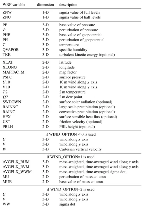
In terms of direct relevance to driving FLEXPART, WRF is a non-hydrostatic mesoscale model that uses perturbation equations with respect to a dry hydrostatic base state. Some of the meteorological variables required by FLEXPART are calculated from a base value and a perturbation from the WRF output (Table 1). WRF uses pressure based terrain-following coordinates. The prognostic variables in WRF are mass-weighted and therefore help to conserve mass.
The WRF pre-processing module, WRF Preprocessing System (WPS), sets the computational domain, the geo-graphical projection, and the resolutions both in the horizon-tal and in the vertical, and interpolates the meteorological fields (usually from a global model analysis or forecast) used as initial and boundary conditions. WPS also prepares and reprojects the static data for the runs (including land use and elevation), which usually comes from satellite information. These data should be considered carefully if fine resolution (∼1 km) is required (e.g. Arnold et al., 2012b).
The choice of meteorological data for the initialization, the land surface model, boundary layer scheme, and convection scheme are all important for an accurate WRF and therefore FLEXPART-WRF simulation. Initialization data choices are limited to what is available, especially in a forecast context. Land surface models range from being quite simple to be-ing extremely complex, and have correspondbe-ing data require-ments. In general, interpolating soil moisture from a global model to the WRF grid is not recommended (Di Giuseppe et al., 2011), but other choices add considerable complex-ity. As for the boundary layer, if the turbulent kinetic en-ergy (TKE) from WRF is to be used in FLEXPART (see Sect. 2.5 below), a scheme that provides TKE must be used. At the time of writing, only the Mellor–Yamada–Janjic (Jan-jic, 2002) and Mellor–Yamada–Nakanishi–Niino (Nakanishi and Niino, 2006) schemes provide the required TKE vari-able. The user should also be aware that different PBL schemes calculate the PBL height differently, and then mod-ify FLEXPART-WRF simulations if the height from WRF is to be used in FLEXPART (again, see Sect. 2.5 below). The choice of whether or not to use a convective scheme in WRF depends on the situation. It is generally advisable to use a convective scheme for a horizontal grid spacing larger than 30 km. Convection schemes are in general not designed for grid spacing less than 10 km, and hence convection should be resolved explicitly by the model. This, however, requires a resolution of 1–2 km or less. There is no general rule for intermediate grid spacing. However, if a convective scheme is used in a WRF domain, a convective scheme should be used in FLEXPART as well, in order to parameterize sub-scale convection.
2.2 FLEXPART-WRF
FLEXPART-WRF v3.1 can handle the different map tions WRF is able to work with. Figure 1 presents the projec-tions that are commonly used in WRF: Lambert conformal, stereographic and Mercator. The blue grid cells represent the center grid of the Arakawa C-grid used in WRF (Fig. 2). The green and red grids represent the two different FLEXPART output projections (see Sect. 2.7 for further details).
Table 1.List of variables needed from the WRF output to run FLEXPART-WRF.
WRF variable dimension description
ZNW 1-D sigma value of full levels ZNU 1-D sigma value of half levels
PB 3-D base value of pressure P 3-D perturbation of pressure PHB 3-D base value of geopotential PH 3-D perturbation of geopotential
T 3-D temperature
QVAPOR 3-D specific humidity
TKE 3-D turbulent kinetic energy (optional)
XLAT 2-D latitude
XLONG 2-D longitude
MAPFAC_M 2-D map factor PSFC 2-D surface pressure U10 2-D 10 m wind alongxaxis V10 2-D 10 m wind alongyaxis
T2 2-D 2 m temperature
Q2 2-D 2 m dew point
SWDOWN 2-D surface solar radiation (optional) RAINNC 2-D large scale precipitation (optional) RAINC 2-D convective precipitation (optional) HFX 2-D surface sensible heat flux (optional) UST 2-D friction velocity (optional) PBLH 2-D PBL height (optional)
if WIND_OPTION≤0 is used
U 3-D wind alongxaxis
V 3-D wind alongyaxis
W 3-D Cartesian vertical velocity
if WIND_OPTION=1 is used
AVGFLX_RUM 3-D mass-weighted, time-averaged wind alongxaxis AVGFLX_RVM 3-D mass-weighted, time-averaged wind alongyaxis AVGFLX_WWM 3-D mass-weighted, time-averaged sigma dot MU 2-D perturbation of mass column
MUB 2-D base value of mass column
if WIND_OPTION=2 is used
U 3-D wind alongxaxis
V 3-D wind alongyaxis
WW 3-D sigma dot
of air by resolved winds are the horizontal and vertical wind 3-D fields. The latitude and longitude 2-D fields are used to validate the projection calculation in FLEXPART. The map factor field is used to correct the displacement of the tra-jectories. The pressure 3-D field is used for density calcula-tions and vertical coordinate transformacalcula-tions. The geopoten-tial is used to interpolate the WRF vertical coordinate onto the FLEXPART vertical coordinate. The specific humidity and temperature 3-D fields are used for calculating air den-sity and different parameters used in PBL parameterizations. The surface pressure, horizontal winds at 10 m a.g.l., the
tem-perature and dew point at 2 m a.g.l. are used to calculate dif-ferent parameters used in PBL schemes.
Some variables are optional. For instance,RAINNC and
RAINCare not necessary for running FLEXPART-WRF with passive tracers; however, they are needed to calculate wet de-position. The output time interval (how often WRF output is provided to FLEXPART) should in general be as short as practical. Brioude et al. (2012b) have shown, for instance, that a time interval of 1 h is reasonable in complex terrain.
Fig. 1.Lambert conformal, Mercator and polar stereographic pro-jections from WRF (blue grid). Two types of projection can be de-fined for the FLEXPART output: A projection that follows the WRF projection output (green grid), the so-called irregular output grid, and a projection based on regular latitude/longitude coordinates (red grid), the so-called regular grid. See Sect. 2.7 for further details on the FLEXPART output.
Fig. 2.Top: Arakawa C grid representing the staggering of the wind field (U, V , W) andT,qv, TKE at the center of the grid. Bottom:
terrain-following coordinates used in WRF (σ) and FLEXPART (z). WRF fields are interpolated vertically onto the terrain following Cartesian coordinate z in subroutine verttransform.f90
2.2.1 User input file
The FLEXPART-WRF model has a somewhat different structure than the FLEXPART-ECMWF/GFS version. In the FLEXPART-WRF, all the input files have been merged into a single control file (See, for instance, flexwrf.testcase0 in the Supplement). The format of the input file has descrip-tions of the different input needed so that experienced FLEX-PART users may easily identify thepathnames(the path name of the directory where the meteorological data and FLEXPART output are located),COMMAND(the list of op-tions), AGECLASSES (the ageclasses used in the exper-iment), OUTGRID (the coordinates and vertical levels of the FLEXPART output domain),RECEPTORS(the coordi-nates of the receptors),SPECIES(a list of species that in-clude molar weight, and wet and dry deposition parameters),
RELEASES(coordinates of the release boxes) files used in FLEXPART-ECMWF/GFS, and can easily adapt scripts if needed. A similar structure, following a namelist, is planned for future versions of FLEXPART-ECMWF/GFS.
file to have any user-defined name; this improves flexibility and helps automatic scripting. The input file has a free for-mat except for the definition of the species used. However, attention has to be paid to the real or integer format required for the input values. Different input files covering different test cases are provided with the source code in the examples directory. A README file is given in the examples direc-tory that describes the purpose of each input file in detail. To run those test cases, the WRF output files can be downloaded from the http://www.flexpart.eu website or from the Supple-ment. FLEXPART-WRF outputs for each of these cases are also included.
Beside the regular switches found in FLEXPART-ECMWF/GFS, new additional switches are available in FLEXPART-WRF. Two new switches allow the user to con-trol the use of the input wind field information. Switch
WIND_OPTIONfacilitates the choice of instantaneous wind with the Cartesian vertical velocity W (option 0), time-averaged wind (option 1), instantaneous wind with eta dot as vertical velocity (option 2) or using a divergence based ver-tical velocity calculated in FLEXPART-WRF (option−1). It is recommended to use option 1. See Sect. 2.3 for further details. A second option, TIME_OPTION, can be used to correct the reference time of the time-averaged wind fields compared to the other instantaneous fields of WRF if not cor-rected by a preprocessing program.
The switchSFC_OPTION allows the user to select dif-ferent treatment of certain PBL and surface parameters, in-cluding PBL height, surface sensible heat flux, and friction velocity. With option 1, these parameters are taken directly from WRF; with option 0 they are diagnosed by FLEXPART. There is no particular recommendation since the PBL height out of WRF might have large uncertainties.
The switch TURB_OPTION allows the use of different PBL turbulence parameterization schemes. Option 1 uses the Hanna scheme used in FLEXPART-ECMWF/GFS. The switchCBLcan be used to assume skewed rather than Gaus-sian turbulence in the convective boundary layer. Options 2 and 3 use the turbulent kinetic energy (TKE) from WRF. Fig-ure 3 presents the vertical profile of the concentration of a passive tracer released from a point source near the surface in a convective PBL after 3 h of transport. In a convective PBL, the tracer is expected to be well mixed throughout the depth of the PBL after such a long transport time. While the tracer using the Hanna scheme and the skewed option CBL is nearly well mixed vertically, the schemes that use TKE from WRF show an unrealistic buildup of tracer near the PBL top. This might be due to an underestimation of TKE near the top of the PBL, the perfect reflection scheme used at the top of the PBL, or an overestimate of the PBL height (from WRF) to be used with TKE. Based on Brioude et al. (2012b) and Fig. 3, it is recommended that one use option 1, as it is, so far, the only option that conserves the well mixed criterion in the PBL.
0 5 10 15 20 25 30 35 40
0 500 1000 1500 2000 2500
concentration(ng/m3)
altitude (m)
Vertical profile of tracer mixing ratio after 3 hours of transport
Hanna scheme CBL scheme TKE scheme
Fig. 3.Vertical profile of concentration of a tracer emitted from a point source at the surface in a convective PBL after 3 h of transport. Vertical profiles from each available PBL scheme in FLEXPART-WRFv3.1 are shown.
The switchRELEASE_COORDchanges the coordinates in which FLEXPART release boxes are specified. This can be in meters, as given in the WRF grid coordinate system (option 0), or as latitude/longitude (option 1).
The switchOUTGRID_COORDlets the user decide on the projection to be used for the FLEXPART-WRF output. Op-tion 0 uses the WRF projecOp-tion, while opOp-tion 1 generates a regular latitude-longitude grid. The definition of the out-put domain, the formerOUTGRIDfile, uses coordinates ac-cording toOUTGRID_COORD. See the test cases for further details.
2.2.2 Parallelization aspects
hourly averaged output fields of 0.25◦resolution. Of course, the number of particles needed in a FLEXPART experiment depends on the size of the domain, the resolution (in space and time) of the meteorological data and the FLEXPART out-put, and the distribution of the sources.
Trivial parallelization can be easily programmed by using several FLEXPART instances in different processors. Note, though, that these runs must be independent from each other (i.e. using different random number sequences). However, treatment of the same meteorological fields in every FLEX-PART instance can amount to a substantial computational overhead, as can the post-processing (e.g. merging) of the output files. Therefore, and to simplify the post-processing, a real parallel version of FLEXPART was desired.
FLEXPART-WRF was programmed keeping the end-user needs in mind; it was intended for a range of different com-putational resources, from single CPU computers to multi-thread clusters with distributed memory. The source code thus consists of some common routines for both parallel and serial runs, and some specific routines either for se-rial or for parallel compilation. The later include the main skeleton FLEXPART routines that control all the integration times and routine calls, the interpolation of the meteorologi-cal fields to the particle positions and, of course, the initial-ization and transport of the particles. The interpolation from the WRF coordinates onto FLEXPART coordinates, the con-centration calculations, and the trajectory integrations have all been parallelized in OPENMP compiler directives for par-allel programming. The reading of the WRF input file could be parallelized as well using a special Network Common Data Form (NetCDF) library that handles parallel reading. However, this has not been implemented yet. Routines with OPENMP instructions do not have a specific name, since the compiler will interpret the OPENMP instructions only when OPENMP is used. Routines marked by thempilabel, how-ever, are the specific routines that use Message Passing In-terface (MPI) parallel programming in distributed memory. This mainly concerns thetimemanager.f90routine and routines that distribute the memory among the nodes within the system. Hence, the user can use OPENMP and MPI to re-duce the computation time needed to perform a FLEXPART-WRF experiment.
The random numbers are handled similarly to the way in which they are in the standard serial FLEXPART; a series of Gaussian random numbers is first generated and stored in memory, and subsequently used during the simulation. In the parallel code, independent Gaussian random numbers series are generated and stored for different MPI processes. This is achieved using different initial seeds coupled with the ran-dom number generator RANLUX (Luscher, 1994; James, 1994). If properly set, this generator theoretically ensures that different seeds create independent random series, which is not true for most generators. Two methods (using the op-tionnewrandomgenin par_mod.f90 line 249) are available for picking the Gaussian random numbers from each series:
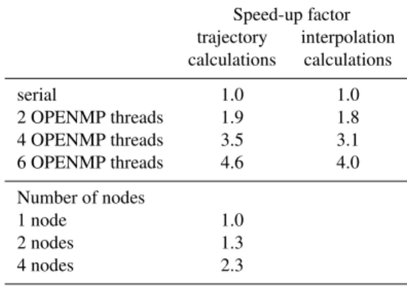
Table 2.Speed factors expected on the trajectory and interpolation calculations using different number of OPENMP threads, and on the trajectory calculations for different number of nodes using MPI threads in hybrid mode. The total speed-up factor in hybrid mode can be calculated by multiplying the speed factors for OPENMP and MPI. See the text for further details.
Speed-up factor trajectory interpolation calculations calculations
serial 1.0 1.0
2 OPENMP threads 1.9 1.8 4 OPENMP threads 3.5 3.1 6 OPENMP threads 4.6 4.0
Number of nodes
1 node 1.0
2 nodes 1.3
4 nodes 2.3
one very quick but less rigorous, and one ensuring a high level of randomness. In the quick method, the series of Gaus-sian random numbers is partitioned based on the number of OPENMP threads, and each thread serially extracts a series from its own partition. This method is very fast but the re-sulting random number series are repetitive with a short pe-riod. In the rigorous method, every OPENMP process has its own independent, uniform random number generator based on the parallel Mersenne–Twister algorithm of Matsumoto and Nishimura (1998), Haramoto et al. (2008) as imple-mented by K. I. Ishikawa (http://www.math.sci.hiroshima-u. ac.jp/~m-mat/MT/VERSIONS/FORTRAN/fortran.html). In this method, any OPENMP process can generate an inde-pendent, uniformly distributed random number whenever re-quired, and use it to randomly select one of the Gaussian dis-tributed numbers previously stored in memory. In this sec-ond case, the algorithm ensures the same level of random-ness as in a single serial FLEXPART simulation; no repet-itiveness should be observed within the resulting series of Gaussian numbers generated for any OPENMP process and no correlation should be observed between streams in dif-ferent OPENMP processes. Of course, the statistical error of the simulation decreases by increasing the number of parti-cles used for each release box (which is true for any Monte Carlo simulation). To achieve a bias of approximately 0.1 % or less in the random term used in the trajectories, we suggest using at least 1000 particles per FLEXPART release location. See the test cases for example.
The user can control the number of cores used by OPENMP by setting the system variable
by (1) the time needed to read the WRF output and inter-polate them onto the FLEXPART vertical coordinate, and (2) the number of trajectories used in the simulation. The larger the number of trajectories, the smaller the statistical sampling errors of the FLEXPART-WRF output. The opti-mization factors in Table 2 are given for the parallelization of the trajectory loop (in timemanager_mpi.f90) and the interpolation/concentration calculations (in
verttransform.f90 and calcpar.f90). The opti-mization of the trajectory calculations will largely determine the time needed to perform a FLEXPART-WRF experiment with a large number of particles. The optimization of the interpolation/concentration calculations will determine the time needed to perform a FLEXPART-WRF run with a large input/output (e.g. using a large computational domain with dense grid spacing and/or many nests). However, since the reading process is not currently parallelized, the effective reduction of computation time will also be determined by the reading of the meteorological input data. These benchmark values are indicative only, since they depend on the com-puter system used. Our OPENMP tests were performed for different numbers of cores using a Xeon E31 225 processor with eight cores. Using OPENMP, the speed-up factor can be expected to be on the order of∼4.6 using 6 cores. The overall speed-up factor (i.e., including the reading process of the WRF output) will depend on the time resolution of the input data, the size of the WRF domain, the time step used in FLEXPART-WRF and the number of trajectories.
The node-to-node intercommunication for MPI instances depends strongly on the connection speed between the nodes. The benchmark for the OPENMP+MPI experiments in Ta-ble 2 was made on a system with Gigabit ethernet connec-tions. Each node had 12 cores. We limited our tests to four nodes, which is probably a typical value for such a FLEX-PART experiment. Our test was made with 40 million tra-jectories, a number typically needed for simulating forward plumes of anthropogenic pollutants over a large domain. Us-ing four nodes, the overall speed-up time usUs-ing MPI together with 6 OPENMP threads (including reading process and in-terpolation) was about 10.
2.3 Ingestion of the meteorological data
Like FLEXPART-ECMWF/GFS, FLEXPART-WRF defines the computational domain, characteristics and grid specifi-cations from the input meteorological data. In the case of a nested input configuration, the coarsest and largest domain will be the one defining the geographical extent of the com-putational domain. WRF output can come in different pro-jected coordinate systems. FLEXPART-WRF uses the same horizontal coordinates as WRF. Thexandycoordinates are given in meters from the lower left corner of the WRF output domain.
FLEXPART-WRF reads the projection informa-tion to convert the WRF coordinates given in meters into latitude/longitude coordinates if necessary (i.e. if release boxes or output grid are defined in geo-graphical coordinates). FLEXPART-WRF uses the
cmapf_mod.f90 and wrf_map_utils.f90 mod-ules and map_proj_wrf.f90 routines to convert back and forth between WRF coordinates (in meters) and lati-tude/longitude coordinates for Lambert conformal, polar stereographic, Mercator, and latitude/longitude projections. FLEXPART-WRF tests the uncertainty in the projection transformation before beginning the experiment using lati-tude and longilati-tude 2-D fields from WRF. FLEXPART-WRF terminates if the error is larger than 2 % of the horizontal grid spacing.
Unlike in FLEXPART-ECMWF/GFS, no singularities are expected at the pole, as WRF should be used with a polar stereographic projection if a pole is included in the domain. Hence, in contrast to the FLEXPART-ECMWF/GFS version, there is no specific treatment of the wind or coordinates near the pole.
Unlike PILT, map factors are used in FLEXPART-WRF to convert the displacement of the particles from the physical displacement on Earth to the WRF domain in
advance.f90. While the grid distances1xand1yin the WRF domain are constant within the WRF domain, the cor-responding distances on Earth are not. Therefore, 2-D map factors are used to calculate the true horizontal distance on Earth at any point in the WRF domain. The Lambert confor-mal, polar stereographic and Mercator projections in WRF are isotropic, which means that the map factors alongx and ydirections are identical. However, map factors alongxand y directions differ for the latitude/longitude projection used for a WRF run at global scale. Map factor (MAPFAC_M) or map factors alongxandydirections (MAPFAC_MX, MAP-FAC_MY) are read from WRF output.
2.4 Vertical interpolation and wind conversion
The WRF model output is on a Arakawa C-grid with terrain-following pressure based sigma levels (also called eta level in WRF manual), where the horizontal and vertical wind components are defined on a staggered grid (Fig. 2). In FLEXPART-WRF, the winds are interpolated onto the grid cell center so that all the meteorological data are on the same grid. Therefore, no external preprocessing of the WRF output is needed.
a near surface level with the wind speed at 10 m a.g.l., and the 2 m temperature and the 2 m specific humidity read in from the WRF output. This option is not recommended if the first sigma level of a WRF run is below 10 m in altitude.
Brioude et al. (2012b) have shown that large uncertainties can arise from usingW, the vertical wind in Cartesian co-ordinates that is output from WRF by default, when signifi-cant orography is encountered in the domain. This version of FLEXPART-WRF therefore gives the possibility to use dif-ferent vertical velocities, and allows choosing between time-averaged and instantaneous winds. Depending on the choice, FLEXPART-WRF will require additional output fields from WRF.
By default, the WRF output includes instantaneous hori-zontal wind alongx andy axes on sigma levels (U andV, in m s−1) and a geometric Cartesian vertical velocity (W, in m s−1). To convertW from a geometric vertical coordi-nate onto a terrain-following coordicoordi-nate (either Cartesian or σ coordinate), a correction factor based on the gradient of orography has to be applied. This is expressed in the form of Eq. (1), whereHis the orography from the WRF output and wthe terrain-following vertical velocity.
w=W−U∂H
∂x −V
∂H
∂y . (1)
If the WRF registry is modified, WRF can output an in-stantaneous mass-weighted sigma dot vertical velocity (WW,
˙
σ in s−1).σ˙ and time-averagedσ˙ follows the same conver-sion as the vertical time-averaged wind.
w= ˙σ ∂z
∂σ
x,y,t
+U ∂z ∂x
y,σ,t
+V ∂z ∂y
x,σ,t + ∂z
∂t
x,y,σ
with Z=z+H. (2)
The last term on the right-hand side of the equation is negligible. The corrective terms (second and third terms) in Eq. (2) are much smaller in magnitude than those from Eq. (1). Using the instantaneousσ˙therefore reduces the mass conservation issues encountered when using the geometric Cartesian vertical velocity (Brioude et al., 2012b).
Since WRF version 3.3, an option allows the user to output mass-weighted, time-averaged winds on sigma lev-els (AVGFLX_RUM, AVGFLX_RVM, AVGFLX_WWM). Time average winds reduce the uncertainty of off-line La-grangian trajectories because the time-mean wind is more representative for the average transport during a given time interval than the rather noisy instantaneous wind. The im-provement owing to the use of time-averaged winds com-pared to instantaneous winds will depend on the meteoro-logical situation and the time interval of the WRF output. See Brioude et al. (2012b) for a comparison between instan-taneous and time-averaged winds as input for FLEXPART-WRF.
The mass-weighted winds are converted to uncoupled winds by applying a mass factor (MU and MUB). The time-averaged vertical wind is a mass-weighted time aver-ageσ˙, and therefore its vertical coordinate transformation in FLEXPART-WRF is equivalent to the one applied on the in-stantaneousσ˙ in Eq. (2).
Since the time-averaged winds are integrated over the WRF time interval output, they are valid at timet−0.51t, with1tbeing the WRF time interval output, andtbeing the valid time of the WRF output. The user has the possibility of setting the switchTIME_OPTION=1 to let FLEXPART correct the valid time of the time-averaged wind internally. If the WRF output has been preprocessed and the valid time of the time-averaged wind is correct,TIME_OPTION=0 has to be used.
If instantaneousσ˙ or time-averaged winds cannot be found in WRF output, FLEXPART-WRF can determine the vertical velocity internally based on mass-conservation and the hy-drostatic assumption. While this assumption is not necessar-ily true at the mesoscale, Brioude et al. (2012b) have found that the uncertainties of this divergence-based vertical veloc-ity are much smaller than those ofw.
Brioude et al. (2012b) have shown that usingσ˙ instanta-neous velocities or time-averaged sigma dot velocities lead to lower wind divergences and thus better results than Carte-sian vertical velocity. The authors argue that there are two possible reasons for the larger errors when usingw. The first one is thatw cannot be accurately converted into a terrain-following vertical velocity due to the partial derivative terms of orography in Eq. (1), which has significant uncertain-ties. In the case ofσ˙, on the other hand, the correction fac-tor involves only the horizontal differences in geopotential between two terrain-following coordinates. The second rea-son might come from the fact that the mass-weightedwis a prognostic variable, while the mass-weighted σ˙ is a di-agnostic variable. The prognostic mass-weighted w might be more sensitive to numerical errors thanσ˙. For more de-tails the reader is referred to the original work by Brioude et al. (2012b) and Nehrkorn et al. (2010). The conversion to the FLEXPART internal vertical coordinate system is made in routine verttransform*.f90 and the routines in-clude the dependency on the vertical wind velocity selected by the user (Fig. 2).
2.5 Boundary layer treatment and turbulence
as in FLEXPART-ECMWF/GFS. Different PBL schemes in WRF calculate the boundary layer height differently, so the user must be aware of these differences ifSFC_OPTION=1
is used. Like in FLEXPART-ECMWF/GFS, the user can decide if an additional term based on subgrid–scale varia-tion of topography and local Froude number will be used in the PBL height calculation. With switch SUBGRID=1, the subgrid variation (envelope PBL height) is used. See Stohl et al. (2005) for further details on the envelope PBL height. The use of this subgrid parameterization is not rec-ommended for mesoscale WRF simulations (horizontal grid spacing≤∼10 km).
Unlike FLEXPART-ECMWF/GFS, FLEXPART-WRF has four different options for the turbulent wind parameterization in the PBL:
– TURB_OPTION=0: Turbulence is completely switched off and FLEXPART works as a non-dispersive Lagrangian trajectory model.
– TURB_OPTION=1: FLEXPART-WRF internally calculates PBL turbulent mixing using the Hanna turbulence scheme (Hanna, 1982). This scheme is based on boundary layer parameters PBL height, Monin–Obukhov length, convective velocity scale, roughness length and friction velocity. These param-eters are either read from WRF or calculated within FLEXPART. Different turbulent profiles are used for unstable, stable or neutral conditions in the PBL. The switch CBL=1 can furthermore be used to assume skewed rather than Gaussian turbulence in the convec-tive PBL. In this case, the CBL formulation of Luhar et al. (1996), extended to account for the gradient in air density formulated by Cassiani et al. (2013), is used for the drift term in the Lagrangian stochastic equation. This drift is based on a skewed proba-bility density function (PDF constructed as a sum of two Gaussians distributions. The formulation assumes that the third moment of vertical velocity in convective conditions has the profile proposed by Luhar et al. (2000) and uses a transition function to modulate the third moment from the maximum possible values in fully convective conditions to zero in neutral conditions. In the present implementation a steady and horizontally homogeneous drift term is used even for unsteady and non-homogenous conditions as done in the standard FLEXPART drift. However, the skewed PDF drift seems to be more sensitive to this inconsistency and a re-initialization procedure of particle velocities has been introduced to avoid numerical instability (Cassiani et al., 2013). If selected, the CBL option requires shorter time steps (typically values of CTL=10 and IFINE=10 are used in the command section of the input file) than the standard Gaussian turbulent model in any case. With the computational time per time step being about
2.5 times that of the standard Gaussian formulation the CBL options is, therefore, much more computa-tionally demanding. It is important to note that the CBL formulation smoothly transitions to a standard Gaussian formulation when the stability changes, but the actual equation solved inside the model for the Gaussian condition is still different from the one used in the standard FLEXPART turbulent option, since, in this equation, it is not the scaled velocity to be advanced, but the actual particle velocity. Full details of the CBL implementation can be found in Cassiani et al. (2013).
– TURB_OPTION=2: The turbulent wind components are computed based on the prognostic turbulent kinetic energy (TKE) provided by WRF. TKE is partitioned between horizontal and vertical components based on surface-layer scaling and local stability with the Hanna scheme.
– TURB_OPTION=3: TKE from WRF is used but the TKE is partitioned by assuming a balance between production and dissipation of turbulent energy.
TURB_OPTION=2 and TURB_OPTION=3 have been tested and found to violate the well-mixed criterion which states that a homogeneously mixed tracer in PBL should stay homogeneously mixed. This is especially a problem in complex terrain. The authors therefore advise using
TURB_OPTION=1.
Above the PBL, turbulence is based on a constant verti-cal diffusivity ofDz=0.1 m2s−1in the stratosphere, follow-ing Legras et al. (2003), and a horizontal diffusivityDh=
50 m2s−1in the free troposphere. See Stohl et al. (2005) for
further details.
2.6 Dry and wet removal processes
smoothing, that, apart from the underestimation of the pre-cipitation maxima, generates events in which a particle could encounter precipitation not associated with a precipitating cloud and thus, according to the FLEXPART-ECMWF/GFS version 8.0–9.02 implementation, would not undergo scav-enging.
A second problematic issue is that this approach overlooks the existence of convective precipitation occurring within subscale and unresolved convective clouds and thus under-estimates the in-cloud scavenging. In FLEXPART-WRF the same issues needed to be addressed, but were adapted to the differences in temporal and horizontal resolutions and to the different disaggregation of the cumulative precipitation fields provided by WRF.
Seibert and Arnold (2013) developed and implemented a better wet deposition scheme for the mainstream FLEXPART-ECMWF/GFS. In FLEXPART-WRF the same approach is taken and adapted to the particular needs of this version. This new scheme includes:
1. The 3-D cloud fraction from WRF is not used and does not mask the scavenging process.
2. The 3-D clouds are diagnosed differently. An initial value of 90 % in relative humidity is taken as a thresh-old for cloud existence, and to obtain the cloud base and height. If precipitation exists but no cloud is diag-nosed, the relative humidity threshold is reduced recur-sively by 5 % incrementation until a cloud is detected. If the relative humidity goes down to 30 %, the precip-itation is mainly convective and FLEXPART detects only a cloud with a 6 km top, then FLEXPART reas-signs the cloud thickness according to the precipitation intensity – from 0.5 km to 8 km for weak precipitation, and from 0 km to 10 km for heavy precipitation. 3. Cloud base and top are interpolated to the particle
po-sition. Neighbor grid cells without diagnosed clouds are not considered in the interpolation.
4. If no cloud is diagnosed, but precipitation exceeding a minimum rainfall rate is present, the bulk parameter-ization previous to version 8 is used with hard-coded scavenging coefficients (by default, aerosol scaveng-ing coefficients).
5. Subgrid variability has been removed from FLEXPART-WRF.
A new study (Seibert and Philipp, 2013) improved the wet deposition scheme by modifying wet scavenging co-efficients. The aerosol lifetime of radionuclides with this new scheme has been evaluated using measurements from the Comprehensive nuclear Test Ban Treaty network in the FLEXPART-ECMWF/GFS model. Improvement in the aerosol lifetime compared to wet deposition has been char-acterized. More investigations on the wet and dry depo-sition schemes are still needed. Dry depodepo-sition follows
the same parameterization used in the latest version of FLEXPART-ECMWF/GFS. To simulate dry removal pro-cesses, FLEXPART-WRF needs to read additional land use and roughness length data available in the data directory where the source directory is located. Those files should be copied or linked into the same directory in which the FLEXPART-WRF binary is used.
2.7 Model output
Three choices of format are given to the user for the FLEXPART-WRF model output. First the user can output in-dividual trajectory information (particle position in space and time, mass of species carried) by using the switchIPOUTto track individual particles. This option is also used for contin-uing a previous FLEXPART-WRF run by reading the infor-mation on the last position of each particle. The output can be formatted in ASCII or as a binary file.
The second choice is to output the center of mass and clus-tered particle positions with additional information (percent-age of tropospheric air, PBL height, etc.) by using the switch
IOUT=4 or 5. The results can be found in the trajecto-ries.txt file in the FLEXPART-WRF output directory and are only available in ASCII format.
The third choice is to distribute the information from each particle onto a regular grid using a uniform kernel. In FLEXPART-WRF, the uniform kernel is not used dur-ing the first 2 h after the particle’s release in order to pre-vent smoothing in the vicinity of the source. This 2 h thresh-old is also applied to the gridded deposition, and for both the single and the nested domain configurations. The grid-ded output is an efficient format for comparing FLEX-PART results to measurements or other model results. The FLEXPART-WRF gridded output can be given in various units, for instance, as a concentration, a volume mixing ratio, or a source-receptor sensitivity (for backward trajectories). The switches IND_SOURCEandIND_RECEPTORcan be used to (1) modify the unit of the quantity released and (2) change the unit of the gridded output following the de-scription by Seibert and Frank (2004).
The output grid coordinates can be defined using the co-ordinate of the lower left corner and the number of grid cells and either the resolution of the gridded FLEXPART-WRF output (switch OUTGRIDDEF=0) or the coordinate of the upper right corner (switchOUTGRIDDEF=1).
Two possibilities are given for the projection of the gridded output. The FLEXPART-WRF output can be de-fined following the WRF projection using the switch
and latitude of the FLEXPART-WRF output can be obtained from the latlon.txt (coordinates of the center grid) and lat-lon_corner.txt (coordinates of the lower left corners) files in the output directory or in the header file if NetCDF format is used.
The second possibility is to define a FLEXPART-WRF output with regularly spaced latitudes and longitudes using the switchOUTGRID_COORD=1(red grid in Fig. 1). In this case, an interpolation is needed to apply the uniform kernel on a latitude/longitude grid. The associated numerical inac-curacies can be potentially important in a polar projection. However, it is the easiest option for comparing FLEXPART-WRF and FLEXPART-ECMWF/GFS results, or to use when-ever output on a latitude/longitude grid is needed.
The FLEXPART-WRF gridded output is formatted either as a binary file or as a NetCDF file. The binary format is compressed by FLEXPART using a custom-designed algo-rithm which dramatically reduces the size of the sparse ma-trix data if there are many zero values. It follows the same format as FLEXPART-ECMWF/GFS output. Fortran, Mat-lab and Python reading routines are avaiMat-lable for reading in the FLEXPART output. Further information is given at http://www.flexpart.eu. The NetCDF format uses NetCDF-4 libraries to compress the NetCDF FLEXPART-WRF out-put files. A header file is generated that includes the lati-tude and longilati-tude coordinates and information on the sim-ulation. A switch,NCTIMEREC, can be used to increase the number of time frames in a single NetCDF file. A NetCDF FLEXPART-WRF output file can include wet and dry depo-sition fields, concentration, mixing ratio fields and source– receptor relationship depending on the type of simulation or species used. Adding more time frames in NetCDF files reduces the overall disk space needed by the NetCDF FLEXPART-WRF output. The compression of the NetCDF file is similar to the binary format if NetCDF library version 4 is used. Using NetCDF library version 3 or earlier versions, the size of the output files is at least 4 times larger.
3 Installation, compilation and execution
FLEXPART-WRF is coded following the Fortran 95 stan-dard, including module options. It has been tested with the Portland Group Fortran compiler, the Intel Fortran com-piler, and the free GFORTRAN compiler in serial, OpenMP, and hybrid OpenMP-MPI modes. FLEXPART-WRF directly reads the WRF output without the need of any external pre-processors. WRF output is commonly given in a NetCDF format and therefore, FLEXPART-WRF requires compila-tion with NetCDF libraries that can read WRF output. To benefit from the compression capability of FLEXPART-WRF NetCDF output format, FLEXPART-WRF has to be linked to a NetCDF-4 library.
The Fortran subroutine par_mod.f90 is used to give the maximum dimension of different variables in the model. Prior to compilation, the user needs to modify the maximum dimensions of the WRF input files at line 126, the maxi-mum number of nests and their maximaxi-mum horizontal dimen-sion at line 160, and the maximum number of species used in FLEXPART-WRF at line 211. Unlike FLEXPART v9.02 or earlier versions, FLEXPART-WRF does not need to have a maximum number of particles. The model automatically handles the number of particles released for each experiment to save memory space.
A single makefile is provided, makefile.mom, which pro-vides the user with a ready-to-work makefile for any of the combinations mentioned above once the user has adapted the library path to her or his own computational environment. This helps inexperienced users with installation and compi-lation, and requires no in-depth knowledge of compilers and compiler options.
The FLEXPART-WRF model can be compiled in three dif-ferent versions. The serial version does not require a specific library besides a NetCDF library and can be compiled by us-ing the followus-ing:
make -f makefile.mom serial
The second version is an OPENMP parallel version that uses more than one core to run the code in shared memory (single PC or single node). This version should be used on any personal computer that has a multi-core CPU (Central Processing Unit) and requires compiler libraries that support multi-threading in shared memory. This version is compiled by using the following:
make -f makefile.mom omp
The third version is a hybrid parallel version that uses MPI and OPENMP. The system needs MPI libraries to be installed beside those that support shared multi-threading. This ver-sion can be used on a super computer, a cluster of PCs or any system that has distributed memory. We recommend using one MPI task per node, and using OPENMP for the multi-threading in shared memory. This version is compiled by us-ing the followus-ing:
make -f makefile.mom mpi
If a module is modified (e.g. par_mod.f90 or com_mod.f90), or if a different version (serial, omp or mpi) needs to be compiled, the object files have to be cleaned before compilation using the following:
make -f makefile.mom clean
A FLEXPART-WRF experiment can be run using an input file named flexwrf.input.forward1 using the fol-lowing command:
flexwrf31_pgi_mpi flexwrf.input.forward1
4 Visualization tool
The FLEXPART-WRF binary output format follows the same format as FLEXPART-ECMWF/GFS version. NCAR Graphics based on fortran, matlab subroutines and python subroutines can be used to read and generate plots from FLEXPART output. The software pflexible (https:// bitbucket.org/jfburkhart/pflexible) written in python provides a set of easily modifiable scripts, allowing the plotting of gridded output, such as concentrations at different vertical levels and deposition fields in single or nested output do-mains. The reader is referred to http://www.flexpart.eu for further details and latest improvement.
The NetCDF FLEXPART-WRF output format can be read and displayed using common visualization tools.
5 Conclusions
The official FLEXPART versions released so far have in-gested input data from the global ECMWF or GFS mod-els. While several derivations of FLEXPART exist, which allow using mesoscale model output, this paper has de-scribed the first official FLEXPART-WRF release. As both WRF and FLEXPART have large user communities, we are confident that this development will be of interest for many atmospheric scientists. The possibility to use input from mesoscale meteorological models for dispersion calcu-lations opens a wide range of possibilities. Like FLEXPART-ECMWF/GFS, FLEXPART-WRF has been released under the GNU GPL and is made available at the new website http://www.flexpart.eu. Future updates will also be available from this website, which facilitates collaborative work by the FLEXPART developers. Users of the FLEXPART model are encouraged to register at this website and make their devel-opments available to others, too. Future develdevel-opments would include the following:
– Adapt reading and transformation subroutines to other mesoscale models.
– Use of snow, 3-D cloud information, land use and soil information from WRF in deposition processes. – Wet and dry deposition and differences among nests
being further tested.
– Continue the work on using turbulence and boundary layer parameters from WRF. The use of the TKE 3-D field from WRF would help to resolve the problem of defining the PBL height.
– Implement new convective schemes or use WRF out-put of entrainment/detrainment to estimate redistribu-tion of particles by subscale convecredistribu-tion instead of us-ing a convective scheme.
– Implement more sophisticated kernel methods, such as a Gaussian kernel, to reduce the smoothing effect of the kernel that can be large at high resolution.
– Include non-stationary and horizontally non-homogenous drift terms in the stochastic equations.
Supplementary material related to this article is available online at http://www.geosci-model-dev.net/6/ 1889/2013/gmd-6-1889-2013-supplement.zip.
Acknowledgement. Jerome Fast and Richard Easter were supported by the US Department of Energy (DOE) Atmospheric System Research Program under Contract DE-AC06-76RLO 1830 at PNNL. PNNL is operated for the US DOE by Battelle Memorial Institute.
Edited by: P. Jöckel
References
Angevine, W. M., Eddington, L., Durkee, K., Fairall, C., Bianco, L., and Brioude J.: Meteorological model evaluation for CALNEX 2010, Mon. Weather Rev., 140, 3885–3906, doi:10.1175/MWR-D-12-00042.1, 2012.
Angevine, W. M., Brioude, J., McKeen, S., Holloway, J. S., Lerner, B. M., Goldstein, A. H., Guha, A., Andrews, A., Nowak, J. B., Evan, S., Fischer, M. L., Gilman, J. B., and Bon, D.: Pollutant transport among California regions, J. Geo-phys. Res., 118, 6750–6763, doi:10.1002/jgrd.50490, 2013. Arnold, D., Vargas, A., Montero, M., Dvorzhak, A., and Seibert, P.:
Comparison of the dispersion model in RODOS-LX and MM5-V3.7-FLEXPART (V6.2), a case study for the nuclear power plant of Almaraz, Hrvatski Meteoroloski Casopis (Croatian Me-teorological Journal), 43, 485–490, 2008.
Arnold, D., Morton, D., Schicker, I., Seibert, P., Rotach, M. W., Horvath, K. J., Dudhia, T. S., Muller, M., Angl, G. Z., Takemi, T., Serafin, S., Schmidli, J., and Schneider, S.: Report on the HiR-CoT 2012 Workshop, 21–23 February 2012, BOKU-MET Re-port, Vienna, Austria, available at: http://www.boku.ac.at/met/ report/BOKU-Met_Report_21_online.pdf (last access: 27 June 2013), 42 pp., 2012a.
Arnold, D., Seibert, P., Nagai, H., Wotawa, G., Skomorowski, P., Baumann-Stanzer, K., Polreich, E., Langer, M., Jones, A., Hort, M., Andronopoulos, S., Bartzis, J., Davakis, E., Kauf-mann, P., and Vargas, A.: Lagrangian Models for Nuclear Stud-ies: Examples and Applications, in Lagrangian Modeling of the Atmosphere, edited by: Lin, J., Brunner, D., Gerbig, C., Stohl, A., Luhar, A., and Webley, P., American Geophysi-cal Union, Washington, DC, doi:10.1029/2012GM001294, pub-lished online first, available at: http://onlinelibrary.wiley.com/ doi/10.1029/2012GM001294/summary, 2012b.
Houston and Dallas, Texas, J. Geophys. Res., 114, D00F16, doi:10.1029/2008JD011493, 2009.
Brioude, J., Kim, S.-W., Angevine, W. M., Frost, G. J., Lee, S.-H., McKeen, S. A., Trainer, M., Fehsenfeld, F. C., Holloway, J. S., Ryerson, T. B., Williams, E. J., Petron, G., and Fast, J. D.: Top-down estimate of anthropogenic emission inventories and their interannual variability in Houston using a mesoscale in-verse modeling technique, J. Geophys. Res., 116, D20305, doi:10.1029/2011JD016215, 2011.
Brioude, J., Petron, G., Frost, G. J., Ahmadov, R., Angevine, W. M., Hsie, E.-Y., Kim, S.-W., Lee, S.-H., McKeen, S. A., Trainer, M., Fehsenfeld, F. C., Holloway, J. S., Peischl, J., Ryerson, T. B., and Gurney, K. R.: A new inversion method to calculate emis-sion inventories without a prior at mesoscale: application to the anthropogenic CO2flux from Houston, Texas, J. Geophys. Res.,
117, D05312, doi:10.1029/2011JD016918, 2012a.
Brioude, J., Angevine, W. M., McKeen, S. A., and Hsie, E.-Y.: Numerical uncertainty at mesoscale in a Lagrangian model in complex terrain, Geosci. Model Dev., 5, 1127–1136, doi:10.5194/gmd-5-1127-2012, 2012b.
Brioude, J., Angevine, W. M., Ahmadov, R., Kim, S.-W., Evan, S., McKeen, S. A., Hsie, E.-Y., Frost, G. J., Neuman, J. A., Pol-lack, I. B., Peischl, J., Ryerson, T. B., Holloway, J., Brown, S. S., Nowak, J. B., Roberts, J. M., Wofsy, S. C., Santoni, G. W., Oda, T., and Trainer, M.: Top-down estimate of surface flux in the Los Angeles Basin using a mesoscale inverse modeling technique: as-sessing anthropogenic emissions of CO, NOxand CO2and their
impacts, Atmos. Chem. Phys., 13, 3661–3677, doi:10.5194/acp-13-3661-2013, 2013.
Brunner, D., S., Henne, S., Kaufmann, P., Schraner, M., and Fuhrer, O.: Development and application of the mesoscale La-grangian particle dispersion model FLEXPART-COSMO, in preparation, 2013.
Cassiani, M., Stohl, A., and Brioude, J.: Lagrangian stochastic mod-elling of dispersion in the convective boundary layer with skewed turbulence conditions and vertical density gradient; mathemati-cal formulation and implementation in FLEXPART, Bound.-Lay. Meteorol, submitted, 2013.
Cooper, O. R., Parrish, D., Stohl, A., Trainer, M., Nedelec, P., Thouret, V., Cammas, J. P., Oltmans, S., Johnson, B., and Tara-sick, D.: Increasing springtime ozone mixing ratios in the free troposphere over western north america, Nature, 463, 344–348, doi:10.1038/nature08708, 2010.
Damoah, R., Spichtinger, N., Forster, C., James, P., Mattis, I., Wandinger, U., Beirle, S., Wagner, T., and Stohl, A.: Around the world in 17 days – hemispheric-scale transport of forest fire smoke from Russia in May 2003, Atmos. Chem. Phys., 4, 1311– 1321, doi:10.5194/acp-4-1311-2004, 2004.
Doran, J. C., Fast, J. D., Barnard, J. C., Laskin, A., Desyaterik, Y., and Gilles, M. K.: Applications of lagrangian dispersion modeling to the analysis of changes in the specific absorp-tion of elemental carbon, Atmos. Chem. Phys., 8, 1377–1389, doi:10.5194/acp-8-1377-2008, 2008.
Draxler, R. R.: HYSPLIT_4 User’s Guide, NOAA Tech. Memo. ERL ARL-230, Air Resources Laboratory, Silver Spring, MD, 35 pp., available at: http://www.arl.noaa.gov/documents/reports/ hysplit_user_guide.pdf (last access: 27 June 2013), 1999.
Fast, J. D. and Easter, R. C.: A Lagrangian particle dispersion model compatible with WRF, 7th WRF Users Workshop, NCAR, 19– 22 June 2006, Boulder, CO, 2006.
Flesch, T. K., Wilson, J. D., and Yee, E.: Backward-time Lagrangian stochastic dispersion models and their application to estimate gaseous emissions, J. Appl. Meteorol., 34, 1320–1332, 1995. Forster, C., Wandinger, U., Wotawa, G., James, P., Mattis, I.,
Althausen, D., Simmonds, P., O’Doherty, S., Kleefeld, C., Jennings, S. G., Schneider, J., Trickl, T., Kreipl, S., Jaeger, H., and Stohl, A.: Transport of boreal forest fire emissions from Canada to Europe, J. Geophys. Res., 106, 22887–22906, doi:10.1029/2001JD900115, 2001.
Forster, C., Cooper, O., Stohl, A., Eckhardt, S., James, P., Dun-lea, E., Nicks Jr., D. K., Holloway, J. S., Huebler, G., Par-rish, D. D., Ryerson, T. B., and Trainer, M.: Lagrangian trans-port model forecasts and a transtrans-port climatology for the Inter-continental Transport and Chemical Transformation 2002 (ITCT 2k2) measurement campaign, J. Geophys Res., 109, D07S92, doi:10.1029/2003JD003589, 2004.
Forster, C., Stohl, A., and Seibert, P.: Parameterization of convec-tive transport in a Lagrangian particle dispersion model and its evaluation, J. Appl. Meteorol. Clim., 46, 403–422, 2007. de Foy, B., Burton, S. P., Ferrare, R. A., Hostetler, C. A., Hair, J.
W., Wiedinmyer, C., and Molina, L. T.: Aerosol plume trans-port and transformation in high spectral resolution lidar mea-surements and WRF-Flexpart simulations during the MILA-GRO Field Campaign, Atmos. Chem. Phys., 11, 3543–3563, doi:10.5194/acp-11-3543-2011, 2011.
de Foy, B., Wiedinmyer, C., and Schauer, J. J.: Estimation of mer-cury emissions from forest fires, lakes, regional and local sources using measurements in Milwaukee and an inverse method, At-mos. Chem. Phys., 12, 8993–9011, doi:10.5194/acp-12-8993-2012, 2012.
Di Giuseppe, F., Cesari, D., and Bonafe, G.: Soil initialization strat-egy for use in limited-area weather prediction systems, Mon. Weather Rev., 139, 1844–1860, 2011.
Gerbig, C., Körner, S., and Lin, J. C.: Vertical mixing in atmo-spheric tracer transport models: error characterization and prop-agation, Atmos. Chem. Phys., 8, 591–602, doi:10.5194/acp-8-591-2008, 2008.
Grell, G. A., Dudhia, J., and Stauffer, D.: A description of the fifth-generation Penn State/NCAR Mesoscale Model (MM5), NCAR Technical Note NCAR/TN-398+STR, doi:10.5065/D60Z716B, 1994.
Hanna, S. R.: Applications in air pollution modeling, in: Atmo-spheric Turbulence and Air Pollution Modelling, edited by: Nieuwstadt, F. T. M. and van Dop, H., D. Reidel Publishing Com-pany, Dordrecht, Holland, 275–310, 1982.
Haramoto, H., Matsumoto, M., Nishimura, T., Panneton, F., and L’Ecuyer, P.: Efficient jump ahead for F_2-Linear Ran-dom Number Generators, Informs J. Comput., 20, 385–390, doi:10.1287/ijoc.1070.0251, 2008.
James, F.: RANLUX: a fortran implementation of the high-quality pseudorandom number generator of Luscher, Comput. Phys. Commun., 79, 111–114, 1994.
Janjic, Z.: Nonsingular implementation of the Mellor–Yamada level 2.5 scheme in the NCEP meso model, NCEP Office Note 437, 61 pp., 2002.
Legras, B., Joseph, B., and Lefvre, F.: Vertical diffusivity in the lower stratosphere from Lagrangian backtrajectory reconstruc-tions of ozone profiles, J. Geophys. Res.-Atmos., 108, 4562, doi:10.1029/2002JD003045, 2003.
Lin, J. C., Gerbig, C., Wofsy, S. C., Daube, B. C., Andrews, A. E., Davis, K. J., and Grainger, C. A.: A near-field tool for simu-lating the upstream influence of atmospheric observations: the stochastic time-inverted lagrangian transport (STILT) model, J. Geophys. Res., 108, 4493, doi:10.1029/2002JD003161, 2003. Luhar, A. K., Hibberd, M. F., and Hurley, P. J.: Comparison of
clo-sures schemes used to specify the velocity pdf in Lagrangian stochastic dispersion models for convective conditions, Atmos. Environ., 30, 1407–1418, 1996.
Luhar, A. K., Hibberd, M. F., and Borgas, M. S.: A skewed mean-dering plume model for concentration statistics in the convective boundary layer, Atmos. Environ., 34, 3599–3616, 2000. Luscher, M.: A portable high-quality random number generator for
lattice field theory simulations, Comput. Phys. Commun., 79, 100–110, doi:10.1016/0010-4655(94)90232-1, 1994.
Matsumoto, M. and Nishimura, T.: Mersenne twister: a 623-dimensionally equidistributed uniform pseudo-random num-ber generator, ACM T. Model. Comput. S., 8, 3–30, doi:10.1145/272991.272995, 1998.
Nakanishi, M. and Niino, H.: An Improved Mellor–Yamada Level-3 Model: Its Numerical Stability and Application to a Regional Prediction of Advection Fog’, Bound.-Lay. Meteorol., 119, 397– 407, 2006.
Nehrkorn, T., Eluszkiewicz, J., Wofsy, S. C., Lin, J. C., Ger-big, C., Longo, M., and Freitas, S.: Coupled weather research and forecasting stochastic time-inverted lagrangian transport (WRF-STILT) model, Meteorol. Atmos. Phys., 107, 51–64, doi:10.1007/s00703-010-0068-x, 2010.
Pagano, L. E., Sims, A. P., and Boyles, R. P.: A Comparative Study between FLEXPART-WRF and HYSPLIT in an Operational Set-ting: Analysis of Fire Emissions across complex geography us-ing WRF, M.Sc. thesis, North Carolina State University, Raleigh, North Carolina, USA, 2010.
Rastigejev, Y., Park, R., Brenner, M. P., and Jacob, D. J.: Resolving intercontinental pollution plumes in global mod-els of atmospheric transport, J. Geophys. Res., 115, D02302, doi:10.1029/2009JD012568, 2010.
Seibert, P. and Arnold, D.: A quick fix for the wet deposition cloud mask in FLEXPART, EGU2013-7922, EGU General Assembly 7–12 April 2013, Vienna, Austria, 2013.
Seibert, P. and Frank, A.: Source-receptor matrix calculation with a Lagrangian particle dispersion model in backward mode, Atmos. Chem. Phys., 4, 51–63, doi:10.5194/acp-4-51-2004, 2004. Seibert, P. and Philipp, A.: The role of deposition in atmospheric
transport of radionucleides, CTBT science and technology con-ference, 17–21 June 2013, Vienna, Austria, 2013.
Seibert, P. and Skomorowski, P.: Comparison of receptor-oriented dispersion calculations based on ECMWF data and nested MM5
simulations for the Schauinsland monitoring station, EGU Gen-eral Assembly, 16–20 April 2007, Wien, 2007.
Skamarock, W. C., Klemp, J. B., Dudhia, J., Gill, D. O., Barker, D. M., Duda, M. G., Huang, X. Y., Wang, W., and Powers, J. G.: A description of the advanced research WRF version 3, Tech. Note, NCAR/TN 475+STR, 125 pp., Natl. Cent. for Atmos. Res., Boulder, Colo., USA, 2008.
Spichtinger, N., Wenig, M., James, P., Wagner, T., Platt, U., and Stohl, A.: Satellite detection of a continental scale plume of ni-trogen oxides from boreal forest fires, Geophys. Res. Lett., 28, 4579–4582, doi:10.1029/2001GL013484, 2001.
Srinivas, C., Venkatesan, R., Muralidharan, N., Das, S., Dass, H., and Kumar, P.: Operational mesoscale atmospheric dispersion prediction using a parallel computing cluster, J. Earth Syst. Sci., 115, 315–332, doi:10.1007/BF02702045, 2006.
Stohl, A. and Thomson, D. J.: A density correction for Lagrangian particle dispersion models, Bound.-Lay. Meteorol., 90, 155–167, 1999.
Stohl, A. and Trickl, T.: A textbook example of long-range trans-port: simultaneous observation of ozone maxima of stratospheric and North American origin in the free troposphere over Eu-rope, J. Geophys. Res., 104, 30445–30462, 1999.
Stohl, A., Wotawa, G., Seibert, P., and Kromp-Kolb, H.: Interpola-tion errors in wind fields as a funcInterpola-tion of spatial and temporal resolution and their impact on different types of kinematic tra-jectories, J. Appl. Meteorol., 34, 2149–2165, 1995.
Stohl, A., Hittenberger, M., and Wotawa, G.: Validation of the La-grangian particle dispersion model Flexpart against large-scale tracer experiment data, Atmos. Environ., 32, 4245–4264, 1998. Stohl, A., Eckhardt, S., Forster, C., James, P., Spichtinger, N., and
Seibert, P.: A replacement for simple back trajectory calcula-tions in the interpretation of atmospheric trace substance mea-surements, Atmos. Environ., 36, 4635–4648, 2002.
Stohl, A., Wernli, H., James, P., Bourqui, M., Forster, C., Lin-iger, M. A., Seibert, P., and Sprenger, M.: A new perspective of stratosphere-troposphere exchange, B. Am. Meteorol. Soc., 84, 1565–1573, 2003a.
Stohl, A., Forster, C., Eckhardt, S., Spichtinger, N., Huntrieser, H., Heland, J., Schlager, H., Wilhelm, S., Arnold, F., and Cooper, O.: A backward modeling study of intercontinental pollution trans-port using aircraft measurements, J. Geophys. Res., 108, 4370, doi:10.1029/2002JD002862, 2003b.
Stohl, A., Cooper, O. R., Damoah, R., Fehsenfeld, F. C., Forster, C., Hsie, E.-Y., Hübler, G., Parrish, D. D., and Trainer, M.: Forecast-ing for a Lagrangian aircraft campaign, Atmos. Chem. Phys., 4, 1113–1124, doi:10.5194/acp-4-1113-2004, 2004.
Stohl, A., Forster, C., Frank, A., Seibert, P., and Wotawa, G.: Technical note: The Lagrangian particle dispersion model FLEXPART version 6.2, Atmos. Chem. Phys., 5, 2461–2474, doi:10.5194/acp-5-2461-2005, 2005.
Thomson, D.: Criteria for the selection of stochastic models of par-ticle trajectories in turbulent flows, J. Fluid Mech., 180, 529–556, 1987.
Warneke, C., Bahreini, R., Brioude, J., Brock, C. A., de Gouw, J. A., Fahey, D. W., Froyd, K. D., Holloway, J. S., Middlebrook, A., Miller, L., Montzka, S., Murphy, D. M., Peischl, J., Ryer-son, T. B., Schwarz, J. P., Spackman, J. R., and Veres, P.: Biomass burning in Siberia and Kazakhstan as an important source for haze over the Alaskan Arctic in April 2008, Geophys. Res. Lett., 36, L02813, doi:10.1029/2008GL036194, 2009.