Performance Evaluation of Affinity Propagation Approaches on Data Clustering

Performance Evaluation of Affinity Propagation

Approaches on Data Clustering

R. Refianti, A.B. Mutiara,

Member IEEE

, and A.A. Syamsudduha

Faculty of Computer Science and Information Technology Gunadarma University

Jl. Margonda Raya No.100, Depok 16424, Indonesia

Abstract—Classical techniques for clustering, such as k-means clustering, are very sensitive to the initial set of data centers, so it need to be rerun many times in order to obtain an optimal result. A relatively new clustering approach named Affinity Propagation (AP) has been devised to resolve these problems. Although AP seems to be very powerful it still has several issues that need to be improved. In this paper several improvement or development are discussed in , i.e. other four approaches: Adaptive Affinity Propagation, Partition Affinity Propagation, Soft Constraint Affinity propagation, and Fuzzy Statistic Affinity Propagation. and those approaches are be implemented and compared to look for the issues that AP really deal with and need to be improved. According to the testing results, Partition Affinity Propagation is the fastest one among four other approaches. On the other hand Adaptive Affinity Propagation is much more tolerant to errors, it can remove the oscillation when it occurs where the occupance of oscillation will bring the algorithm to fail to converge. Adaptive Affinity propagation is more stable than the other since it can deal with error which the other can not. And Fuzzy Statistic Affinity Propagation can produce smaller number of cluster compared to the other since it produces its own preferences using fuzzy iterative methods.

Keywords—Affinity Propagation, Availability, Clustering, Exem-plar, Responsibility, Similarity Matrix.

I. INTRODUCTION

Nowadays, the need of information in many aspects of life is really high. The information need to be delivered fast and accurate. It makes the extraction process of information from data is really crucial. There are many ways in mining an information from data, one of them is clustering. Clustering is commonly used to analyze data which is have very large or even huge data in numbers and the class label on data are unknown. Since assigning class labels to large number of data are very high cost process so then another approach such as clustering is needed to mine useful information from data. The Clustering is focused on finding methods for efficient and effective cluster analysis in large databases [4].

In clustering usually it is need to select some cluster centers to guarantee that the sum of squared errors between each data point and its potential cluster center is small during clustering. Classical techniques for clustering, such as k-means clustering, partition the data into k clusters and are very sensitive to the initial set of data centers, so they often need to be rerun many times in order to obtain a satisfactory result.

A relatively new clustering approach named Affinity Prop-agation (AP) has been devised to resolve these problems [1],

[2]. The AP clustering method has been shown to be useful for many applications in face images, gene expressions and text summarization. Unlike previous methods, AP simultane-ously considers all data points as potential exemplars, and it recursively transmits real-valued messages along edges of the network until a good set of centers is generated. In particular, corresponding clusters gradually emerge in AP.

Since its first appearance it already gain much attention from many researchers. Many research and development re-lated to the affinity propagation had been conducted, such as adaptive affinity propagation [11], relational affinity propa-gation [9], landmark affinity propapropa-gation [10], fuzzy statistic affinity propagation [13] and many more emerged since AP introduced as one of powerful clustering algorithm. Although AP has a better solution in clustering data, but it still has several issues related its performance. So AP is still need and open to great possible improvements.

In order to be able in improving AP performance, a wise step to do it by learning from another AP algorithms that have been proposed. By learning and comparing several algorithm, it is possible to gain more information related to their advantages and disadvantages. Later those advantages can be combined to produce a new and better algorithm while at the same time trying to avoid their disadvantages side.

Problems discussed in this research are restricted as fol-lowing. This research is only meant to find the cluster centers from data images. The data that being used is 2000 data of facial images. And the approaches of affinity propagation that are implemented are only five approaches, i.e. the affinity propagation itself, adaptive affinity propagation [11], partition affinity propagation [12], soft constraint affinity propagation [8], and Fuzzy statistic affinity propagation [13].

The aims of this research are to look for the advantages and disadvantages of affinity propagation development, in order to be able to make a further research to develop a new algorithm which is better and capable to handle clustering faster and more accurate. The research will greatly help a lot of people who is dealing with a large data to make the information extraction easier and faster. Later it is possible for development a new algorithms that can cluster a large data in faster way.

Our paper is organized as follows: In section II, we presents the relevant theories of clustering and its methods, also affinity propagation and its recent developments. Section III, we explains the analysis of affinity propagation and the

application design, and their experiment and analysis results are then presented and discussed in Section IV.

II. LITERATURESTUDY

A. Affinity Propagation

Affinity Propagation is a fast clustering algorithm based on message passing that identifies a set of cluster center that represents the dataset [2]. Since it was proposed and published by Frey and Dueck in a paper Science magazine 2007, it is proven has much better performance and much lower clustering error than existing clustering methods [1]. It can support similarities that are not symmetric or do not satisfy the triangle inequality, and it is deterministic which is its clustering results do not depend on initialization unlike most of clustering methods such as k-means [3]. That means AP has some advantages according to its computational speed, general applicability, and good performance [11].

Affinity Propagation works based on similarities between pairs of data points and simultaneously considers all data points as potential exemplars (cluster centers). AP searches for clusters recursively through an iterative process, real valued messages are transmitted or exchanged between data points until high quality set of exemplars and corresponding cluster emerges. In the iterative process, identified exemplars start from the maximum n number to fewer exemplars until m exemplars appear and unchanging for a certain number of iterations (converges). The m clusters found based on m exemplars are the clustering solution of AP.

Affinity Propagation takes as input a collection of real valued similarities between data points, where the similarity S(i, j)indicates how well the data point with indexj is suited to be the exemplar for data point i. The goal of AP is to minimize the squared error, then each similarity is set to a negative squared error (Euclidean Distance). For data pointxi andxj :

S(i, j) =−|xi−xj|2 (1)

In Affinity Propagation there are two kinds of message exchanged between data points, they are Responsibility and Availability (see Fig. 2). The responsibility R(i, j) is sent from data point i to candidate exemplar point j. It reflects the accumulated evidence for how well suited point j is to serve as the exemplar for point i. The availability A(i, j) is sent from candidate exemplar pointj to data pointi. It reflect the accumulated evidence for how appropriate it would be for pointi to choose pointj as its exemplar.

Affinity propagation takes as input a real number S(k, k) for each data point k so that data points with larger values of (S(k, k)are more likely to be chosen as exemplars. These values are referred to as Preferences. The number of identified exemplars (number of clusters) is influenced by the values of the input preferences, but also emerges from the message-passing procedure. The preferences should be set to a common value. This value can be varied to produce different numbers of clusters. The shared value could be the median of the input similarities (resulting in a moderate number of clusters) or their minimum (resulting in a small number of clusters).

Fig. 1: Similarity Between Data Points [2]

Fig. 2: Responsibility and Availability [2]

When updating the messages, it is important that they be damped to avoid numerical oscillations that arise in some circumstances. Each message is set to λ times its value from the previous iteration plus 1−λtimes its prescribed updated value, where the damping factor λis between 0 and 1.

In each iteration of affinity propagation consisted of up-dating all responsibilities given the availabilities, upup-dating all availabilities given the responsibilities, and combining avail-abilities and responsibilities to monitor the exemplar decisions and terminate the algorithm when these decisions did not change for certain number of iterations.

B. Affinity Propagation Developments

Currently there are many research related to the clustering algorithms of Affinity Propagation. Here will be reviewed several of them. They are Adaptive Affinity Propagation, Parti-tion Affinity PropagaParti-tion, Soft Constraint Affinity PropagaParti-tion, Fast Sparse Affinity Propagation [7], Relational Affinity Prop-agation [9], Fuzzy Statistic Affinity PropProp-agation, Patch Affinity Propagation [15], and Fast Affinity Propagation [3].

1) Adaptive Affinity Propagation: Adaptive Affinity Prop-agation is one of the development of affinity propProp-agation algorithm which is developed based on the fact that the original

affinity propagation is still have several issues. Affinity propa-gation is known that its clustering result is really influenced by the initial value of the preference parameter (diagonal values of similarity matrix). Minimum value of preference will drive to a small number of cluster center result, while median value will drive to a moderate result. Then how to know what is the best value to be set on the preference to produce the optimal clustering solution. So this algorithm is designed by Kaijun Wang to overcome this issue [11].

Beside the preference issue there is another issue that this algorithm try to deal with. In some cases, the occurrence of os-cillations can not be avoided. Oscillation is a condition where the identified exemplar is keep changing in each iteration which is caused the process is fail to reach convergence. And if it made into a graph, the graph will show a periodic graph. The requirement of convergence is that the exemplar is not changing for certain amount of iteration. On original affinity propagation when the oscillation occurs then the clustering process is failing so it is need to be rerun with increasing the damping factor values. But there is a fact that the greater value of damping factor the slower the process will take times.

Adaptive Affinity Propagation divided into three main parts. The first part is called Adaptive Damping which is the process of adjusting the damping factor to eliminate oscilla-tions adaptively when the oscillaoscilla-tions occur. The second part is called Adaptive Escape which is the process of escaping the oscillations by decreasing the preferences value when adaptive damping method fails. And the last part is called Adaptive Preference Scanning which is the process of searching the space of preferences to find out the optimal clustering solution to the data set.

2) Partition Affinity Propagation: Partition Affinity Propa-gation is an extension of affinity propaPropa-gation which can reduce the number of iterations effectively and has the same accuracy as the original affinity Propagation [12]. This extension comes at the cost of making a uniform sampling assumption about the data. Partition affinity propagation passes messages in the subsets of data first and then merges them as the number of initial step of iterations, it can effectively reduce the number of iterations of clustering.

In each iteration of affinity propagation the updating of each responsibility R(i, j) takes availabilities and similarities between data points into consideration, while the updating of availability A(i, j) has a relationship with responsibilities between other data points. Therefore, given the similarity col-lection, the clustering result achieved by AP is the same with the same preference value as input. However, initial availability matrix is also a factor which will lead to different identified exemplar set [14]. To produce different identified exemplar set by changing initial availabilities matrix of AP. This algorithm reduces the time spent by decreasing the number of iterations by decomposing the original similarity matrix into submatrices

3) Soft Constraint Affinity Propagation: Soft Constraint Affinity Propagation is one of the development of affinity propagation algorithm which is developed based on the fact that the original affinity propagation is still suffers from a number of drawback. The hard constraint of having exactly one exemplar per cluster restricts AP to classes of regularly shaped clusters, and leads to suboptimal performance [8].

Each point in the cluster on AP refers to exemplar, and each exemplar is required to refer to itself as a self-exemplar. This hard constraint forces clusters to appear as stars of radius one. There is only one central node, and all other nodes are directly connected to it. The hard constraint in AP relies strongly on cluster shape regularity, elongated or irregular multi-dimensional data might have more than one simple cluster center.

This problems may be solved by modifying the original optimization task of AP. This softening of hard constraint is using a finite penalty term for each constraint violation.

4) Fuzzy Statistic Affinity Propagation: Fuzzy Statistic Affinity Propagation [13] is one of the development of affinity propagation algorithm which is developed based on fuzzy statistics. Fuzzy statistics is a combination of statistical meth-ods and fuzzy set theory. Fuzzy set theory is the basis in studying membership relationships from the fuzziness of the phenomena. Fuzzy statistics is used to estimate the degree of membership of a pattern to a class according to the use of a membership function. At the Fuzzy Statistic Affinity Propagation compute fuzzy mean deviation and then develop a fuzzy statistical similarity measure (FSS) in evaluating the similarity between two pixel vectors before running the AP iterative process.

III. RESEARCHMETHODOLOGY

A. System Analysis

In order to conduct research about clustering by Affinity Propagation, there are several steps that have to be considered and to be done. These steps are data collection, data prepro-cessing, similarity matrix construction, evidence calculation, and cluster exemplar identification.

1) Data Collection: Data collection is the very first step to do in cluster analysis. In this research, data are searched and collected through internet. The data are consists of 250x250 pixels 8500 facial images which is collected from 1500 living people category on Wikipedia [5]. These data has been widely used in several researches such as mining faces biographies [6]. But in this research only 2000 facial images will be used. Here are several samples of the images.

Fig. 3: Sample Data Images [5]

2) Data Preprocessing: Before the collected data pro-ceeded to the clustering process, these data are needed to be preprocessed first to eliminate noise and irrelevant information. These steps include image cropping, image resizing, and image gray scaling.

3) Similarity Matrix Construction: After the data are com-pletely preprocessed. it is needed to extract the histogram from the images. this histogram will be used and subtracted with another histogram from the other images to measure its similarities. to do that, a distance approaches called Negative Euclidean Distance is used to handle it. Below is the formula of negative Euclidean distance.

−|xi−xj|2 (2)

According to the Euclidean distance the diagonal matrix should be equal to zero, since it is being subtracted from itself. These zero values need to be replaced with another values. This values later will be called as the preferences value. This preference value later will influences the clusters output and the number of cluster. it is one of the crucial parameter in affinity propagation. Different value will cause different cluster result. It can be said that the number of identified clusters is increased or decreased by adjusting preference value correspondingly [11].

There are two options that usually are chosen to set the preference value, by setting it to its median from similarity matrix median(S) or the other hand is setting it to its minimum min(S). The median value will lead to a moderate number cluster result, while the minimum result in a small number of cluster. Beside these two options a custom value can also be set if it possibly can give a better cluster solution.

4) Evidence Calculation: Evidence calculation is the main part of affinity propagation which is all the computation take place. It is divided into two main parts. The first one is called Responsibility Update, and the second is Availability Update. The responsibility R(i, j) reflects the accumulated evidence for how well suited point j is to serve as the exemplar for pointi. While the availabilityA(i, j)reflects the accumulated evidence for how appropriate it would be for point i to choose pointj as its exemplar.

First will be illustrated how to compute the responsibility update from the similarity matrix. But before that it is need to be predefined some parameters such as set the maximum iteration number, convergence iteration, and damping factor. For the first iteration make sure that the availability is set to zeroA(i, j) = 0.

The Responsibility Update itself is based on these formula.

R(i, j) =

S(i, j)−max{A(i, j) +S(i, j)} (i6=j) S(i, j)−max{S(i, j)} (i=j)

(3)

To gain an understanding about how the responsibility update actually works, here is presented the algorithm of Responsibility Update.

To illustrate the above algorithm, the first step is adding the similarity matrix with the initial Availability which is now zero for the first iteration. In the next iteration it will no longer remain zero, some of it will be replaced by negative of positive number.

AS(i, j) =A(i, j) +S(i, j) (4)

Algorithm 1 . Responsibility Update Calculation

Input : Simmilarity Matrix S(i, j), Availability Matrix A(i, j),

Maximum Iteration, Convergence Iteration, Damping Factor

Output : Responsibility Matrix R(i, j)

1: Set Matrix R(i, j) = 0 and A(i, j) = 0 (first iteration only)

2: ComputeAS(i, j) =A(i, j) +S(i, j)

3: Compute max value and record the index [maxV al(i), Index] =max(AS)

4: Replace max value with max negative real number/inf AS(Index) =−inf

5: Compute 2nd max value[maxV al2(i)] =max(AS) 6: Make vector max into matrix maxAS(i, j) =

repmat(maxV al(i))

7: Replace max Value Index with 2nd max Value maxAS(Index) =maxV al2(i)

8: Substract S with maxASR(i, j) =S(i, j)−maxAS(i, j) 9: Compute finalR(i, j) = (1−lam)∗R(i, j)−lam∗R(i, j)

Then find the maximum values from the matrixAS(i, j). And record the index locations.Replace the maximum values with any other value that will always be the greatest value of all values in the matrix. In this case it can be replaced by an infinite number or real maximum number. This is meant to make sure that those index will no longer chosen as the maximum value in the matrix so it can chose the second maximum values. Since the negative value of infinite number of real maximum number will always become the smallest number. With the replaced maximum values, we find the second maximum values from the matrix.

Make a new matrix with the same size as matrixAS(i, j) from the first maximum values. Replace some values according to the recorded index from the first maximum values with the second obtained maximum values.

Then subtract the similarity matrixS(i, j)with the matrix maxAS(i;j)and then will be obtained a new matrix which is called responsibility matrix R(i, j). Below is the substraction process.

R(i, j) =S(i, j)−maxAS(i, j) (5)

And the last step is to multiply the obtained matrix with the damping factor. This damping factor will be really useful later to prevent an oscillation which is will cause the algorithm to fail to reach a convergence. Convergence itself is the condition where the identified number of cluster is no longer changing for certain number of iteration which is called as convergence iteration. And the formula of damping factor is like follow.

R(i, j) = (1−λ)·R(i, j)−λ·R(i, j) (6)

The damping factor (λ) value can be set between zero to one. In this illustration the value is set to 0.5. And finally the final responsibility matrix is obtained like below. This matrix will be the input for the availability update.

The second main part of affinity propagation is to calculate the availability matrix which is called Availability Update. The

input of this step is still the same as the previous one plus the new matrix responsibility. Availability update process is based on these formula

A(i, j) =

_{min(0,(R(j, j) +}P_{max(0, R(i, j)))) (i6=j)} P

max(0, R(i, j)) (i=j) (7)

To gain an understanding about how the availability update actually works, here is presented the algorithm of Availability Update.

Algorithm 2 . Availability Update Calculation

Input : Responsibility Matrix R(i, j)

Output : Availability MatrixA(i, j) 1: FindRp(i, j) =R(i, j)>0

2: Put diagonalR(i, j)to diagonalRp(i, j) 3: Compute sum ofRp(i, j)

4: Make new matrix fromsum(Rp(i, j))

5: Compute matrixA(i, j) =sum(Rp(i, j))−Rp(i, j) 6: FindA(i, j)<0

7: Put diagonalA(i, j)to diagonalA(i, j)<0

8: Compute finalA(i, j) = (1−lam)∗A(i, j)−lam∗A(i, j)

To illustrate the algorithm above, here used the previous calculated responsibility matrix as the input. The first step is to find the values within responsibility matrix which is greater than zero. Then put the value of diagonal responsibility matrix to the new matrix. This new matrix then is called as respon-sibility preference Rp(i, j) matrix. From this matrix add all values in the same column to produce a vector responsibility.

Make a new matrix from this vector that will be used later to be subtracted by matrix responsibility preference. Subtract this matrix with matrix responsibility preference Rp(i, j) to produce matrix Availability A(i, j)). Then from this matrix AvailabilityA(i, j)look for the values that have smaller values than zero. The values from diagonal of availability matrix is placed to the diagonal of new matrix availability then the final availability matrix will be formed.

And the last is the same like responsibility matrix, multiply it with the damping factor as shown below.

A(i, j) = (1−λ)·A(i, j)−λ·A(i, j) (8)

5) Cluster Exemplars Identification: In order to be able to identify an exemplars or cluster centers from the similarity matrix using affinity propagation there are two things that need to be created, they are the responsibility and availability matrix. At the previous explanation, both of responsibility and availability is successfully created. These two matrixes later will determine the clustering result. To identify the cluster centers, it simply just need to add both matrix responsibility and availability like follow.

C(i, j) =R(i, j) +A(i, j) (9)

From this matrix C(i, j) the cluster centers easily deter-mined by looking for the value that greater than zero. These whole process from the responsibility update until cluster

identification will be done repeatedly until the number of identified cluster is unchanging for certain amount of times.

B. Affinity Propagation Analysis

Previously it is already described the whole system of affinity propagation and how it is actually works. Now in this part will be presented some of the developments related to the affinity propagations. They are Adaptive Affinity Propagation, Partition Affinity Propagation, Soft Constraint Affinity Propa-gation Algorithm, and Fuzzy Statistic Affinity PropaPropa-gation.

Algorithm 3 . Adaptive Damping and Escape

Input : Monitoring Windoww= 40, Damping Factorlam= 0.5,

Maximum Iterationmaxits, Preference StepP s

Output : Exemplars of Each Data Points 1: fori= 0 toi= 10do

2: Record IdentIFied ExemplarsKset(i) =K 3: ifi > w/8 then

4: ComputeKmean(i) =mean(Kset(i−(w/8) :i)) 5: Check FOR Decreasing K

6: ifKmean(i)−Kmean(i−1)<0 then

7: K Decreased is trueKd= 1

8: end if

9: Check FOR Uchanging K

10: ifKset(i)−Kset(i−1) == 0then

11: K changed is TrueKc= 1 12: end if

13: Check FOR non-oscillation 14: ifKd== 1orKc== 0 then

15: Kb(i) = 1 16: end if

17: Check FOR Oscillation Occurance 18: ifsum(Kb)<2/3wthen

19: Activate Adaptive Damping

20: Increase damping factorlam+ 0.05 21: iflam >0.85 then

22: Activate Adaptive Escape 23: Icrease PreferenceP+P s

24: end if

25: end if 26: end if

27: end for

1) Adaptive Affinity Propagation Algorithm: In adaptive affinity propagation proposed a method called Adaptive Damp-ing which is the process of adjustDamp-ing the dampDamp-ing factor to eliminate oscillations adaptively when the oscillations occur. The second part is called Adaptive Escape which is the process of escaping the oscillations by decreasing the preferences value when adaptive damping method fails.

In adaptive damping method when the oscillations oc-cur, the damping factor will be increased automatically or adaptively once by a step such as 0.05. But after increasing the damping factor until certain number such as 0.85 and the oscillations is still occur then it is used adaptive escape method to deal with it. The adaptive escape is activated if the adaptive damping fail to handle the oscillation by increasing the preference values of similarity matrix until the process reach convergence.

Algorithm 4 . Partition Affinity Propagation

Input : Number of Data PointN,Similarity Matrix S(i, j)

Output : Exemplars of Each Data Points

1: Calculate Number of PartitionN part=sqrt(N)/2 2: Calculate Matrix Partition SizeP artSize=N/N part 3: Set Partition End point to zeroEndP = 0

4: fori= 1 toN partdo

5: Calculate Partition Start PointStartP = 1+P artSize∗ (i−1)

6: ifi==N partthen

7: Calculate Matrix SizeP artSize=N−P artSize∗ (N P art−1)

8: Calculate Partition End Point EndP = EndP + P artSize

9: else

10: Calculate Partition End Point EndP = EndP + P artSize

11: end if

12: Contruct Sub Matrix SM(i, j) = S(StartP : EndP, StartP :EndP)

13: Run Resposibility Update Once with matrixSM(i, j) 14: Run Availability Update Once and save inSubA(i) 15: end for

16: Combine All obtainedA(i, j) =SubA(∗) 17: Run Affinity Propagation with NewA(i, j)

Algorithm 5 . Soft Constraint Affinity Propagation

Input : Simmilarity MatrixS(i, j), Soft Constraint PenaltyP

Output : Exemplars of Each Data Points 1: Compute Responsibility Update

2: Campare diagonal value of matrix R(i, i) = max(−P, R(i, i))

3: Compute Avalailability Update

4: Campare diagonal value of matrix A(i, i) = min(P, A(i, i))

2) Partition Affinity Propagation Algorithm: Partition affin-ity propagation is an extention of affinaffin-ity propagation which can reduces the time spent to find the exemplar by decreasing the number of iterations. It can be achieved by decomposing the original similarity matrix into sub-matrices. This algorithm passes messages in the subsets of data first and then merges them as the number of initial step of iterations, it can ef-fectively reduce the number of iterations of clustering. The Algorithm is stated as follow.

3) Soft Constraint Affinity Propagation Algorithm: Soft Constraint Affinity Propagation is one of the development of affinity propagation algorithm which is developed based on the fact that the original affinity propagation is still suffers from a number of drawback. Each point in the cluster on AP refers to exemplar, and each exemplar is required to refer to itself as a self-exemplar. This hard constraint forces clusters to appear as stars of radius one. This problems may be solved by modifying the original optimization task of AP. This softening of hard constraint is using a finite penalty term for each constraint violation. The Algorithm is stated as follow.

4) Fuzzy Statistic Affinity Propagation Algorithm: Fuzzy Statistic affinity propagation is an extension of affinity

prop-Algorithm 6 . Fuzzy Statistic Affinity Propagation

Input : Number of Data N, Data Points X, exemplar Z, membership degreeU,

degree of fuzzinessB, error rateE, Cluster Threshold ScalarCT S

Output : Similarity MatrixS(i, j), and PreferenceP 1: Set values ofB,E, andCT S

2: Set initialU = 1, fuzzy mean distance f mdist= 0, and stopping conditionstop= 0

3: Calculate fuzzy distancef dist=|X−Z| 4: whilestop== 0 do

5: Record old fuzzy mean distancef mdist1 =f mdist 6: Calculate fuzzy mean distancef mdist= (f dist∗U)/U 7: Calculate fuzzy distance deviation f dev = f dist −

f mdist

8: Calculate fuzzy mean distance deviation f mdev = (f dist−f mdist)/N

9: Calculate membership degree U =

exp((−f devB_{)/(f mdev}B₎₎

10: Calculate stopping conditionsc=f mdist1−f mdist 11: ifsc < E then

12: stop= 1 13: end if

14: end while

15: Calculate fuzzy similarity matrixS(i, j) =−f mdist 16: Calculate preference P = min(S(i, j)) −

CT S(max(S(i, j)−min(S(i, j))))

agation based on fuzzy statistic and AP. It simultaneously considers all data points in the feature space to be initial clustering exemplars and iteratively refines with the mean distance deviation until getting the optimal fuzzy statistical similarity matrix.The Algorithm is stated as follow.

IV. RESULTS ANDDISCUSSIONS

Affinity Propagation algorithms is implemented in MAT-LAB programming environment. Data Preprocessing is a pro-cess to eliminate noise and irrelevant information from data. The steps include image cropping, image resizing, and image gray scaling.

The first test result of affinity propagation which is the original algorithm of affinity propagation. It shows that the number of identified cluster centers or exemplars are 6 exem-plars from 2000 images with 134 iteration in 23.9285 seconds. From the adaptive affinity propagation algorithm is identified the number of cluster centers or exemplars from 2000 images are 7 exemplars with 247 iteration in 43.3825 seconds. Below is the detailed information including graph and log application.

From the partition affinity propagation algorithm is iden-tified the number of cluster centers or exemplars from 2000 images are 7 exemplars with 119 iteration in 21.0428 seconds. The soft constraint affinity propagation seems like not giving any result since it is fail to meet a convergence.Below is the detailed information including graph and log application.

From the fuzzy statistic affinity propagation algorithm is identified the number of cluster centers or exemplars from 2000 images are 3 exemplars with 64 iteration in 13.3443

TABLE I: Log Mininum Result of Original and Adaptive AP

Original AP Adaptive AP

Number of Data 2000 200

Total Iteration 134 249

Total Identifier. Cluster 6 7

Cluster Exemplar 559, 900, 173, 213, 1069, 1074, 606,769, 1304, 1555 1369, 1633, 1859 Cluster Exemplar Index 900, 1304, 1369, 173, 900, 1304, 1369, 213, 559, 559 608, 1633, 769 Execution Time 23.9265 sec. 43.3825 sec.

Fig. 4: Graph Minimum Original Affinity Propagation Result

Fig. 5: Graph Minimum Adaptive Affinity Propagation Result

TABLE II: Log Mininum Result of Partition and Soft-Constraint AP

Partition AP SC AP

Number of Data 2000 2000

Total Iteration 119 179

Total Identifier. Cluster 7

-Cluster Exemplar 380, 559, 1069, — 1074, 1095, 1497

1555

Cluster Exemplar Index 1095, 380, 1095, – 380, 559, 559

Execution Time 23.9265 sec. —

Fig. 6: Graph Minimum Partition Affinity Propagation Result

Fig. 7: Graph Minimum Soft Constraint Affinity Propagation Result

seconds. Below is the detailed information including graph and log application.

TABLE III: Log Mininum Result of Fuzzy-Statistics AP

Fuzzy-Statistic AP

Number of Data 2000

Total Iteration 64

Total Identifier. Cluster 3 Cluster Exemplar 500, 1259, 1770, Cluster Exemplar Index 1297, 1297, 1297, 500, 1770 Execution Time 13.3443 sec.

Fig. 8: Graph Minimum Fuzzy Statistic Affinity Propagation Result

for exemplars from minimum values of preference. The second test result is about to show the identified exemplars from the median values of preferences. the original algorithm of affinity propagation. It shows that the number of identified cluster centers or exemplars are 21 exemplars from 2000 images with 54 iteration in 9.6316 seconds. From the adaptive affinity prop-agation algorithm is identified the number of cluster centers or exemplars from 2000 images are 22 exemplars with 134 iteration in 23.0912 seconds. Below is the detailed information including graph and log application.

TABLE IV: Log Median Result of Original and Adaptive AP

Original AP Adaptive AP

Number of Data 2000 200

Total Iteration 54 134

Total Identifier. Cluster 21 22

Cluster Exemplar 22, 88, 144, 460, 267, 443, 537, 586, 501, 66 634, 672, 685, 725 Cluster Exemplar Index 443, 1333, 685, 634, 1019, 88, 799, 537, 1591, 672, 1729 Execution Time 9.6316 sec. 23.0912 sec.

Fig. 9: Graph Median Original Affinity Propagation Result

Fig. 10: Graph Median Adaptive Affinity Propagation Result

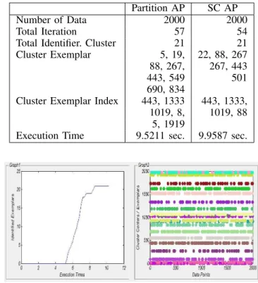
From the partition affinity propagation algorithm is iden-tified the number of cluster centers or exemplars from 2000 images are 21 exemplars with 57 iteration in 9.5211 seconds.

From the soft constraint affinity propagation algorithm is identified the number of cluster centers or exemplars from 2000 images are 21 exemplars with 54 iteration in 9.9587 seconds. Below is the detailed information including graph and log application.

TABLE V: Log Median Result of Partition and Soft-Constraint AP

Partition AP SC AP

Number of Data 2000 2000

Total Iteration 57 54

Total Identifier. Cluster 21 21

Cluster Exemplar 5, 19, 22, 88, 267 88, 267, 267, 443

443, 549 501

690, 834

Cluster Exemplar Index 443, 1333 443, 1333, 1019, 8, 1019, 88

5, 1919

Execution Time 9.5211 sec. 9.9587 sec.

Fig. 11: Graph Median Partition Affinity Propagation Result

Fig. 12: Graph Median Soft Constraint Affinity Propagation Result

From the fuzzy statistic affinity propagation algorithm is identified the number of cluster centers or exemplars from 2000 images are 3 exemplars with 64 iteration in 13.3443 seconds. Below is the detailed information including graph and log application.

To make it easier to compare the clustering result using affinity propagation approaches. We present Table VII and Table VIII that consist of all the testing results.

TABLE VI: Log Median Result of Fuzzy-Statistics AP

Fuzzy-Statistic AP

Number of Data 2000

Total Iteration 84

Total Identifier. Cluster 3 Cluster Exemplar 1159, 1671, 1734, Cluster Exemplar Index 1734, 1734, 1734, 1159, 1671 Execution Time 16.868 sec.

Fig. 13: Graph Median Fuzzy Statistic Affinity Propagation Result

TABLE VII: Testing Result with Minimum Preferences

Algorithms Minimum Preferences Exemplar Iteration Time(s)

Original 6 134 23.9285

Adaptive 7 249 43.3825

Partition 7 119 21.0428

Soft Constraint - -

-Fuzzy Statistic 3 64 13.3443

TABLE VIII: Testing Result with Median Preferences

Algorithms Median Preferences Exemplar Iteration Time(s)

Original 21 54 9.6316

Adaptive 22 134 23.0912

Partition 21 57 9.5211

Soft Constraint 21 54 9.9587

Fuzzy Statistic 3 84 16.868

From the above table original affinity propagation with minimum preferences value generates 6 cluster centers within 23.93 second after 134 iterations, and 21 cluster centers in 9.63 second with 54 iteration for the median preferences. The second algorithm, Adaptive affinity propagation takes much longer time to find the exemplars even compared to the other four approaches it is the slowest algorithm. Slow execution time is the cost of adaptive affinity propagation that has to take since it main goal is to eliminates the possible error occupance. In some cases in the middle of iteration oscillation will occur and causing the algorithm to fail to converge and need to rerun with different parameters value. Adaptive affinity propagation tries to eliminate this error with sacrificing its speed but more

certain in finding cluster centers. From the table the fastest algorithm is the partition affinity propagation that has the fastest execution time 21.04 second for minimum preference and 9.52 second for median preference compared to the other approaches. Partition affinity propagation has a goal to reduce the iteration numbers so the execution time will be faster. Compared to the original affinity propagation which is takes 134 iteration to find 6 exemplars, partition affinity propagation only takes 119 iteration to find 7 exemplars in minimum pref-erences. and partition affinity propagation takes 57 iteration to find 21 exemplars. Soft constraint affinity propagation with the median preference finds 21 exemplars with 54 iterations, the same as the original affinity propagation but slightly slower execution time since in soft constraint affinity propagation in each iteration it is comparing the diagonal matrix with its soft constraint preference (scp). But in the minimum preference the algorithm is fail to converge, it can be caused by the occupance of oscillations or the value of scp is not well set. The last algorithm, fuzzy statistic affinity propagation resulting in the smallest number of cluster centers or exemplars. It finds 3 exemplars in both minimum and median preference since it is generate its own preference using the fuzzy iterative methods. and in the median preference original affinity propagation takes 54 iteration

V. CONCLUDINGREMARKS

According to the testing results, it can be inferred that among several affinity propagation development which is ex-plained in this research Partition Affinity Propagation is the fastest one among four other approaches. Partition Affinity Propagation is slightly faster than the other since it uses an approach to divide matrix into several part to reduce the iteration numbers. On the other hand Adaptive Affinity Propagation is much more tolerant to errors, it can remove the oscillation when it occurs where the occupance of oscillation will bring the algorithm to fail to converge. Adaptive Affinity propagation is more stable than the other since it can deal with error which the other can not. And Fuzzy Statistic Affinity Propagation can produce smaller number of cluster compared to the other since it produces its own preferences using fuzzy iterative methods.

For future work, in order to produce a better algorithm of affinity propagation consider to try combining two or three algorithm compared in this research such as adaptive and partition affinity propagation or any other affinity propagation. So it can run faster and stabler in generating cluster center from massive data.

ACKNOWLEDGMENT

The authors would like to thank the Gunadarma Founda-tions for financial supports.

REFERENCES

[1] D. Dueck, “Affinity propagation: clustering data by passing messages,” Ph.D. dissertation, Citeseer, 2009.

[2] B. J. Frey and D. Dueck, “Clustering by passing messages between data points,”science, vol. 315, no. 5814, pp. 972–976, 2007.

[3] Y. Fujiwara, G. Irie, and T. Kitahara, “Fast algorithm for affinity propagation,” inIJCAI Proceedings-International Joint Conference on Artificial Intelligence, vol. 22, no. 3. Citeseer, 2011, p. 2238.

[4] J. Han, M. Kamber, and J. Pei,Data mining, southeast asia edition: Concepts and techniques. Morgan kaufmann, 2006.

[5] M. K. Hasan and C. Pal, “Experiments on visual information extraction with the faces of wikipedia,” in Twenty-Eighth AAAI Conference on Artificial Intelligence, 2014.

[6] M. K. Hasan and C. J. Pal, “Improving alignment of faces for recognition,” inRobotic and Sensors Environments (ROSE), 2011 IEEE International Symposium on. IEEE, 2011, pp. 249–254.

[7] Y. Jia, J. Wang, C. Zhang, and X.-S. Hua, “Finding image exemplars using fast sparse affinity propagation,” inProceedings of the 16th ACM international conference on Multimedia. ACM, 2008, pp. 639–642. [8] M. Leone, M. Weigtet al., “Clustering by soft-constraint affinity

prop-agation: applications to gene-expression data,”Bioinformatics, vol. 23, no. 20, pp. 2708–2715, 2007.

[9] A. Plangprasopchok, K. Lerman, and L. Getoor, “Integrating structured metadata with relational affinity propagation.” inStatistical Relational Artificial Intelligence, 2010.

[10] P. Thavikulwat, “Affinity propagation: A clustering algorithm for computer-assisted business simulations and experiential exercises,” De-velopments in Business Simulation and Experiential Learning, vol. 35, 2014.

[11] K. Wang, J. Zhang, D. Li, X. Zhang, and T. Guo, “Adaptive affinity propagation clustering,”arXiv preprint arXiv:0805.1096, 2008. [12] D.-y. Xia, F. Wu, X.-q. Zhang, and Y.-t. Zhuang, “Local and global

approaches of affinity propagation clustering for large scale data,” Journal of Zhejiang University SCIENCE A, vol. 9, no. 10, pp. 1373– 1381, 2008.

[13] C. Yang, L. Bruzzone, F. Sun, L. Lu, R. Guan, and Y. Liang, “A fuzzy-statistics-based affinity propagation technique for clustering in multi-spectral images,”Geoscience and Remote Sensing, IEEE Transactions on, vol. 48, no. 6, pp. 2647–2659, 2010.

[14] X. Zhang, F. Wu, and Y. Zhuang, “Clustering by evidence accumulation on affinity propagation,” inPattern Recognition, 2008. ICPR 2008. 19th International Conference on. IEEE, 2008, pp. 1–4.

[15] X. Zhu and B. Hammer, “Patch affinity propagation,”ICOLE 2010, p. 63, 2011.