J. Bremer
Leibniz-Institute of Atmospheric Physics, 18225 K¨uhlungsborn, Schloss-Str. 6, Germany
Received: 10 May 2007 – Revised: 13 November 2007 – Accepted: 13 November 2007 – Published: 28 May 2008
Abstract. Ground based ionosonde measurements are the most essential source of information about long-term varia-tions in the ionospheric E and F1 regions. Data of such ob-servations have been derived at many different ionospheric stations all over the world some for more than 50 years. The standard parametersfoE, h’E, and foF1 are used for trend analyses in this paper. Two main problems have to be con-sidered in these analyses. Firstly, the data series have to be homogeneous, i.e. the observations should not be disturbed by artificial steps due to technical reasons or changes in the evaluation algorithm. Secondly, the strong solar and geo-magnetic influences upon the ionospheric data have carefully to be removed by an appropriate regression analysis. Other-wise the small trends in the different ionospheric parameters cannot be detected.
The trends derived at individual stations differ markedly, however their dependence on geographic or geomagnetic lat-itude is only small. Nevertheless, the mean global trends es-timated from the trends at the different stations show some general behaviour (positive trends infoEandfoF1, negative trend inh’E) which can at least qualitatively be explained by an increasing atmospheric greenhouse effect (increase of CO2 content and other greenhouse gases) and decreasing ozone values. The positive foEtrend is also in qualitative agreement with rocket mass spectrometer observations of ion densities in the E region. First indications could be found that the changing ozone trend at mid-latitudes (before about 1979, between 1979 until 1995, and after about 1995) modi-fies the estimated meanfoEtrend.
Keywords. Atmospheric composition and structure (Ion chemistry of the atmosphere; Thermosphere-composition and chemistry) – Ionosphere (Ionosphere-atmosphere inter-actions; Solar radiation and cosmic ray effects) – Radio sci-ence (Ionospheric propagation; Remote sensing)
Correspondence to:J. Bremer ([email protected])
1 Introduction
Trend analyses with ionospheric data have mainly been initi-ated by model results of Roble and Dickinson (1989) assum-ing a doublassum-ing of the atmospheric greenhouse gases CO2and CH4in the Earth’s atmosphere. Based on these results Rish-beth (1990) and RishRish-beth and Roble (1992) predicted a low-ering of the F2-layer by about 15–20 km and of the E-layer by about 2.5 km. Additionally they prognosticated a decrease of the peak electron density of the F2-layer (decrease of foF2 by about 0.2–0.5 MHz) and an increase of the peak electron density of the F1- and E-layers (foF1increase by about 0.3– 0.5 MHz;foEincrease by 0.05–0.08 MHz). During the fol-lowing years a lot of investigations have been carried out to test these predictions using ionosonde observations at differ-ent stations. Most of these investigations deal, however, with trends in the ionospheric F2-layer (peak height, i.e. hmF2, as well as peak electron density expressed by foF2). A compi-lation of these results can be found in Bremer (2005). Trend analyses with ionosonde parameters of the E- and F1-layer are fewer and mostly restricted to one or a few stations (Bre-mer, 1992; Givishvilli et al., 1995; Sharma et al., 1999). Only some papers deal with the results of more globally dis-tributed stations (Bremer, 1998, 2001, 2004; Mikhailov and de la Morena, 2003; Bremer et al., 2004; Mikhailov, 2006).
In this present paper earlier results of trend analyses with characteristic ionosonde parameters of the ionospheric E-and F1-regions (Bremer, 1998; 2001; 2004) will be updated using data series newly extended to the year 2005. New as-pects of this paper deal with latitudinal and longitudinal vari-ations of the ionospheric trends as well as the influence of ozone variations on these trends.
2 Data analysis and methodical investigations
1190 J. Bremer: Long-term trends in the ionospheric E and F1 regions
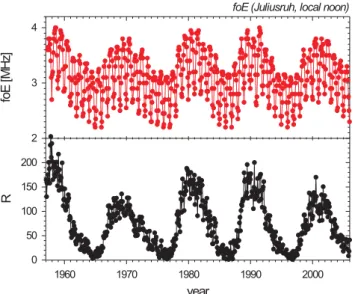
Fig. 1. Long-term variations of monthly meanfoEvalues of the ionosonde station Juliusruh at local noon (upper part) and of solar sunspot numberR(lower part).
foEvalues of the station Juliusruh (54.6◦N; 13.4◦E) are
pre-sented (upper part) together with the solar sunspot number R (lower part). Two things can obviously be remarked, firstly the foE values are markedly dependent on the solar activ-ity and secondly thefoEvalues have a pronounced seasonal variation. Moreover,foEhas also a diurnal variation, not to be seen in Fig. 1 because it is restricted to a fixed time (lo-cal noon). This variability has to be taken into consideration in the trend analyses. Therefore, the elimination of the solar and geomagnetic influences upon the observed parameters Xobs=foE,h’EorfoF1are carried out for each hour and each month separately. At first the solar and geomagnetically in-duced parts of the ionospheric parameter are estimated by the following twofold regression formula
Xt h=a+b·R+c·Ap. (1) Here R is the solar sunspot number as proxy of the solar activity,Apis the global geomagnetic activity index,bandc are the corresponding partial regression coefficients, and a is constant factor describingXt hforR=0 andAp=0. Then the difference between the observed and calculated ionospheric parameters are estimated by
1X=Xobs−Xt h (2)
or the relative differences are calculated
1X=(Xobs−Xt h)Xt h. (3) Trend analyses can be done for each hour and each month separately, but often the1Xdata series are combined to get more representative yearly mean1X values which are also used in this paper to derive linear trends according to
1X=d+e·year. (4)
Fig. 2.Long-term variations of different solar activity indices: solar sunspot numberR, solar 10.7 cm radio flux F10.7, and solar EUV proxy E10.7.
Here the valueeis the trend parameter for the individual sta-tion whereasdis a constant factor for1Xat year=0.
In Eq. (1) the solar sunspot number is used as the solar activity index. It is however also possible to use other in-dices as the solar 10.7 cm radio flux F10.7 or the EUV proxy E10.7 (Tobiska, 2001). In Fig. 2 these three indices are pre-sented for the time period between 1948 and 2005. In spite of some unusually high monthly mean values of the E10.7 index during 1957 all three indices are very strongly corre-lated (e.g. correlation coefficientsr(R, F10.7)=0.975, r(R, E10.7)=0.948). Therefore, the choice of the solar activity in-dex should not be very critical.
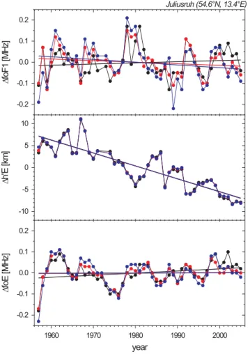
Fig. 3. Long-term trends of different ionospheric parameters (foE,
h’E,foF1) observed at the ionosonde station Juliusruh after elimi-nation of the solar and geomagnetic influences using different solar activity indices (R: black, F10.7: red, E10.7: blue).
As mentioned above the trend analyses can be made with absolute (Eq. 2) or relative differences (Eq. 3). In Fig. 4 one example is shown withfoE trends derived from ionosonde observations at the station Port Stanley (51.7◦S, 57.8◦W) using both methods. The long-term variations of the derived 1foEvalues are very similar and the derived linear trends are nearly identical if we use a meanfoEvalue of 2.2 MHz. Therefore, also the choice of both methods seems to be un-critical. In this present paper absolute differences according to Eq. (2) are used in agreement with earlier papers of the author.
3 Experimental trends from global ionosonde observa-tions
In the following the results of the trend analyses are pre-sented for the different characteristic ionospheric parameters separately. In each case only yearly 1X data series have been investigated to get most reliable data series. These data
Fig. 4.Trends infoEof the ionosonde station Port Stanley derived from absolute (lower part) and relative differences (upper part) be-tween experimental and regression model values.
series have been derived from all1X data series for each month and each hour where observation data are available, i.e. without night-time values forfoE,h’E, andfoF1as well as without winter values forfoF1. Also other missing data (e.g. caused by technical reasons) have not been included in the analyses, e.g. by use of interpolation methods. The length of the individual data series is different reaching from 15 years up to 49 years. The first year of the analysed data is 1957 as in connection with the International Geophysical Year (IGY) a lot of ionosondes started their operation in this year, the last analysed year is 2005.
3.1 Trends infoE
From 71 different globally distributed ionosonde stations in-dividualfoEtrends have been derived. In Fig. 5 these indi-vidual trends are shown in a histogram (right part). Nega-tive values are in red, posiNega-tive values in blue. The signifi-cant trends are in dark colours (confidence level greater than 95%), the non-significant trends (confidence level less than 95%) in light colours. The significance of the individual trends has been tested by the Fisher’s F parameter
F =r2·(n−2).(1−r2). (5) Here r is the correlation coefficient between1Xand year af-ter Eq. (4) and n is the number of years with data. The signif-icance levels for the F parameter can be found in Taubenheim (1969). The median value of the individual trends (marked by the arrow in the histogram) is 0.0011 MHz/year.
1192 J. Bremer: Long-term trends in the ionospheric E and F1 regions
Fig. 5.Global meanfoEtrend (left part) and histogram (right part) deduced from observations at 71 individual ionosonde stations.
Fig. 6. foEtrends in dependence on the absolute value of the lati-tude of the individual stations (upper part) and on the longilati-tude of these stations (lower part). The dashed lines characterize the mean globalfoEtrend, the full lines are the curves of the best linear fit (upper part) and sinusoidal fit (lower part) through the individual trend values.
error of this trend has been calculated with the following for-mula (Taubenheim, 1969)
Error(95%)=tβ(n−2) .p
(n−2)·
r
s2 x
.
s2
y−e21x(y).(6) Here tβ is the threshold value of the Student’s t test with a confidence level of 95%, n the number of years,sx2ands2yare the variances ofX(=foE,foF1, orh’E) and ofy(=year), and e is the regression coefficient (= trend value) from Eq. (4). ForX=foEthe estimated mean error is±0.0005 MHz/year.
Therefore, the mean globalfoEtrend is significantly different from zero. Inside of the left part of Fig. 5 the trend value with error limits is presented including the number n of years used
Fig. 7.Global meanh’Etrend (left part) and histogram (right part) deduced from observations at 33 individual ionosonde stations.
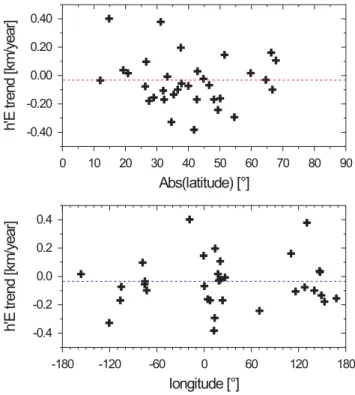
Fig. 8. h’Etrends in dependence on the absolute value of the lati-tude of the individual stations (upper part) and on the longilati-tude of these stations (lower part). The dashed lines characterize the mean globalh’Etrend.
in the mean trend analysis and the correlation coefficientr between1foEand year. Using these values the correspond-ingF parameter according to Eq. (5) can easily be estimated (F=47.9) which demonstrates a strongly significant correla-tion between 1foEand year (confidence level above 99%) thus confirming the result presented above by use of Eq. (6). The derived mean trend in the left part of Fig. 5 agrees rea-sonably with the median value of the individual trends in the right part.
strong variability of the individual trends this result is how-ever an indication of a latitudinal dependence offoEtrends. The correlation between the individual trend values and the corresponding values from the fitted curve (r=0.36) is signif-icant with a confidence level of about 99%.
3.2 Trends inh’E
Trends in the virtual height of the ionospheric E layer,h’E, have been derived from data series of 33 different ionosonde stations. These individual trends are presented in a histogram (right part of Fig. 7). Negative trends are in red, positive in blue. Significant trends are marked by dark colours, non-significant trends by light colours. The median value is
−0.068 km/year.
In the left part of Fig. 7 the mean globalh’Etrend is shown calculated from all 33 individual1h’Edata series. The mean trend is−0.029 km/year and therefore different from the
me-dian value of the individual trends in the right part of Fig. 7. The reason of this difference may be the small number of available stations and the strong differences between the in-dividual trend values producing a relatively disturbed his-togram with some peaks. In spite of the small number of available stations the mean trend is significant with more than 95% confidence as to be seen by the error which is markedly smaller than the mean trend (see numbers in the left part of Fig. 7). This result can be confirmed by the Fisher’sF test. Using the correlation coefficientr and the number of years n as presented in the left part of Fig. 7, a valueF=6.6 can be estimated due to Eq. (5) which demonstrates a significant correlation between1h’Eand year with a confidence level of more than 95%.
The dependences of theh’Etrends on the absolute value of the latitude and on the longitude of the individual ionosonde stations are presented in Fig. 8. There are no remarkable de-pendencies to be seen, probably caused by the limited num-ber of available stations. The dashed lines mark the mean h’Etrend as derived in the left part of Fig. 7.
3.3 Trends infoF1
Similar as above forfoEandh’Ethe trend results forfoF1 observations are presented in Fig. 9. In the right part of Fig. 9 the histogram is presented for the individualfoF1trends with a median value of 0.0021 MHz/year. The positive trends are presented in blue, the negative in red. The significant trends
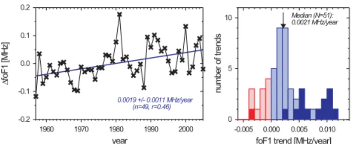
Fig. 9.Global meanfoF1trend (left part) and histogram (right part) deduced from observations at 51 individual ionosonde stations.
are characterized by dark colours, the non-significant trends by light colours.
In the left part of Fig. 9 the mean globalfoF1 trend is shown estimated from the1foF1data series of all 51 avail-able stations. The mean trend with 0.0019 MHz/year agrees reasonably with the median value of all individual trends. As the error limit is markedly smaller than the mean value (see numbers inside the left part of Fig. 9), the derived global trend is significant with more than 95%. This fact can also be confirmed by the calculation of the F value according to Eq. (5) with the r and n values shown inside of the left part of Fig. 9. The estimated valueF=12.6 indicates a significant correlation between1foF1and year with a confidence level of more than 99%.
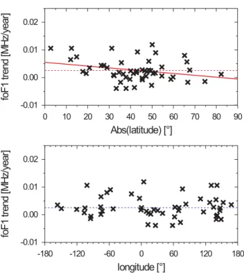
In Fig. 10 the individualfoF1trends are presented in de-pendence on the absolute values of the latitude as well as on the longitude of the available measuring stations. There seems to be a slight tendency thatfoF1trends at low latitudes become stronger similar as also observed in the upper part of Fig. 6 forfoEtrends. The derived slope of the linear regres-sion line (full red line in the upper part of Fig. 11) is due to the Fisher’sFparameter test significant with about 88% con-fidence. There is however no visible dependence of thefoF1 trends on the longitude (lower part of Fig. 10). The dashed lines in both parts of Fig. 10 mark the mean foF1trend as derived in the left part of Fig. 9.
3.4 Influence of ozone on trends infoE
From long-term observation of the total ozone content in the atmosphere over Europe (Krzyscin et al., 2005) peri-ods with different ozone trends can be detected, only small trends before 1979, a marked decrease between 1979 and 1995, and a small ozone increase after about 1995. These features can also be seen in the total ozone data series ob-served at Arosa (coordinates: 46.8◦N, 9.7◦E; data source: M¨ader, 2005, and DWD, 2005) in Fig. 11. After elimination of the solar and geomagnetically induced parts a mean to-tal ozone trend has been derived with−0.44 DU/year for the
1194 J. Bremer: Long-term trends in the ionospheric E and F1 regions
Fig. 10. foF1trends in dependence on the absolute value of the latitude of the individual stations (upper part) and on the longitude of these stations (lower part). The dashed lines characterize the mean globalfoF1trend, the full red line in the upper part is the best linear fit through the individual trend values.
Fig. 11.Long-term variation of total ozone observed at Arosa after elimination of the solar and geomagnetic influences. The red line is the linear trend for the whole interval between 1957 and 2005, the blue lines characterize the trends in different sub-intervals.
Akmaev et al., 2006) that ozone changes may influence not only the stratosphere but also the meso- and lower thermo-sphere. Therefore, it seems to be reasonable to investigate whether the different ozone trends may influence trends in the E region. In Fig. 12 the variation of mean1foEvalues
Fig. 12. Long-term variation offoEdeduced from observations at 45 stations in mid-latitudes (30–60◦N, 30–60◦S) after elimination of the solar and geomagnetic influences. The red line is the linear trend for the whole interval between 1957 and 2005, the blue lines characterize the trends in different sub-intervals.
is shown, here however estimated only from 45 stations at mid-latitudes (30–60◦S and 30–60◦N). The mean trend (red
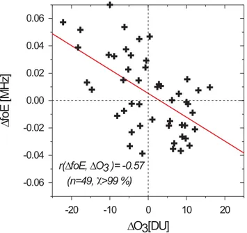
line) is identical with the mean globalfoE trend shown in Fig. 5 (left part). Also the estimated error value is similar to the value for the global trend, thus confirming the high con-fidence level of this long-term trend. ThefoEtrends in the three sub-intervals (blue lines) are quite different with a very small trend before 1979, a steep increase of the trend during the time period between 1979 and 1995, and a reduced trend after 1995. Due to the short length of these sub-intervals the estimated trends can describe only the main features of the1foEvariations and there remain some discrepancies be-tween the trend values at the boundaries of adjacent inter-vals. The confidence levels of these trends are partly very small. Only for the second interval (1979–1995) the confi-dence level is markedly higher than 95%, for the third in-terval this level is only 64% whereas in the first inin-terval the 1foEtrend is nearly zero. Nevertheless there are some simi-larities between the ozone trends in Fig. 11 and the trends in foEin Fig. 12. This statement is confirmed by the correla-tion between1foEvalues from Fig. 12 and1O3data from Fig. 11 presented in Fig. 13 with a significant correlation co-efficientr(1foE,1O3)=−0.57.
4 Discussion
Fig. 13. Correlation between 49 yearly mean values of1foE de-duced from ionosonde observations at mid-latitudes and1O3at Arosa.
Table 1.Mean global trends in different ionospheric parameters. N is the number of ionosonde stations used in the trend analyses.
Region Parameter N Mean exp. trend Error (95%)
F1 foF1 51 0.0019 MHz/year ±0.0011 MHz/year E foE 71 0.0013 MHz/year ±0.0005 MHz/year E h’E 33 −0.029 km/year ±0.020 km/year
with more than 15 years have been used; most of the series are however longer than two solar cycles, extending to 49 years at maximum.
The method used to derive long-term trends has been de-scribed in Section 2 above. As demonstrated there the choice of the solar activity index as well as the method using abso-lute or relative differences between the observed and mod-elled data is uncritical and should not influence the presented trend results markedly. But there is another trend method de-veloped by Mikhailov and de la Morena (2003) which uses quite another algorithm. These authors try to exclude long-term variations of the geomagnetic activity. Their results cannot directly be compared with the results presented in this paper. These authors believe that before about 1970 the long-term variation offoEis mainly controlled by the long-term variation of the geomagnetic activity, after that time, however, afoEincrease should be caused by anthropogenic sources.
In spite of the exclusion of non-homogeneous data series the differences between individual trends in all ionospheric
foE 0.0013 MHz/year 0.26 MHz 0.05. . . 0.08 MHz h’E −0.029 km/year −5.8 km −2.5 km
parameters analysed here are relatively strong as can be seen in the histograms presented in the right parts of Figs. 5, 7, and 9. The reasons for these differences are not quite clear, some of them may be caused by their geographical locations. E.g. there are small indications that thefoEandfoF1trends are more pronounced at low latitudes than at mid- and high latitudes (see upper parts of Figs. 6 and 10), but the confi-dence levels of the corresponding regression lines are small as already remarked above in Sects. 3.1 and 3.3.
1196 J. Bremer: Long-term trends in the ionospheric E and F1 regions
Fig. 14. Long-term variation of CO2 observed at Hawaii. The red line is the linear trend for the whole interval between 1958 and 2004, the blue lines characterize the trends in different sub-intervals.
the reduced NO density as predicted from model calculations for an increasing greenhouse effect (Roble and Dickinson, 1989; Beig, 2000).
One reason for the observed discrepancies between ob-served and modelled data in the E region may result from the fact that in the model calculations of Roble and Dickin-son (1989), Rishbeth (1990) and Rishbeth and Roble (1992) only the trends of the greenhouse gases CO2and CH4have been considered. But also ozone (Bremer and Berger, 2002; Akmaev et al., 2006) as well as water vapour trends (Akmaev et al., 2006) can amplify the modelled trends.
The influence of ozone trends on thefoEtrends is demon-strated in Figs. 11–13 above. The dates of possible trend changes have mainly been derived from long-term ozone changes (Krzyscin et al., 2005). The year 1979 is also sup-ported by stratospheric trend analyses of Labitzke and Nau-jokat (2000) with clearly changing temperature trends at this time. ThefoEtrends in the different sub-intervals in Fig. 12 are of course not only caused by the changing ozone trends but also by the CO2trends. In Fig. 14 the long-term varia-tion of CO2is presented derived from observations at Hawaii (Keeling and Whorf, 2005). Due to these measurements the CO2 trend increases steadily from the interval before 1979 with 1.03 ppmv/year until 1.82 ppmv/year, to the interval af-ter 1995. Therefore, for the explanation of thefoEtrends the influence of different greenhouse gases (CO2, CH4, O3, H2O and others) have to be taken into account. Here it should only be expressed that in agreement with model results (Ak-maev et al., 2006) ozone changes influences also long-term trends in the E region. In the globalh’Etrend the influence of ozone could, however, not be detected, probably due to the markedly reduced data volume (only data from 33 stations and not enough data after 1999).
In the F1 region no influence of ozone changes uponfoF1 trends have been found. Here the influence ozone should also be markedly smaller than in the E region as derived by Akmaev et al. (2006) in their model calculations.
It is not quite clear if the latitudinal variation of thefoE trends in the lower part of Fig. 6 is a real effect or only an artefact. However, the possibility cannot be excluded that the individual trends may depend on their latitude. In solar cycle effects of the temperature in the strato- and mesosphere some zonal asymmetric effects have been found (Hampson et al., 2006). Therefore, in the future this effect has to be investigated in more detail, e.g. for different seasons.
5 Summary and conclusions
Using data series from long-term observations at globally distributed ionosonde stations, the trends of different char-acteristic ionospheric parameters (foE,h’E,foF1) have been derived. The main results can be summarized as follows:
– The detection of relatively small long-term trends in ionospheric data series requires the careful elimination of the strong solar and geomagnetic influences as al-ways mentioned by the author in previous publications and also found by a lot of other investigators. Here a twofold regression analysis is made using different solar activity indices and the global geomagnetic Ap index. – The globally averaged mean trends (positive trends in
foE and foF1, negative h’E trend) qualitatively agree with model calculations of the effect of the increasing atmospheric greenhouse effect. However, the experi-mental trends in the E region are markedly stronger than in the model predictions.
– The derived trends at the individual stations differ markedly. There are some indications of a slight lati-tudinal dependency (stronger trends at lower latitudes infoEandfoF1), however the confidence level is rela-tively low. ThefoEtrend values slightly depend on the longitude with an indication of a simple sinusoidal vari-ation.
– Changes in the mid-latitude total ozone trends modify thefoEtrends. Therefore, stratospheric ozone changes also influence long-term variations in the lower thermo-sphere in qualitative agreement with model results. The extension of the ionospheric data series until 2005 was very helpful for these investigations.
– General remark: In trend analyses it should carefully be checked whether the investigated time interval can be analysed by a simple linear regression line (or another continuous curve) or whether it is more reliable to sub-divide the interval into different sub-periods, especially if there are physical reasons to do it.
Acknowledgements. The author is very grateful to the reviewers A. D. Danilov and M. J. Jarvis for their critical and very helpful remarks and comments to this paper.
105, 19 841–19 856, 2000.
Brasseur, G. and de Rudder, A.: The potential impact on atmo-spheric ozone and temperature of increasing trace gas concen-trations, J. Geophys. Res., 92, 10 903–10 920, 1987.
Bremer, J.: Ionospheric trends in mid-latitudes as a possible indi-cator of the atmospheric greenhouse effect, J. Atmos. Terr. Phy., 54, 1505–1511, 1992.
Bremer, J.: Trends in the ionospheric E and F regions over Europe, Ann. Geophys., 16, 986–996, 1998,
http://www.ann-geophys.net/16/986/1998/.
Bremer, J.: Trends in the thermosphere derived from global ionosonde observations, Adv. Space Res., 28(7), 997–1006, 2001.
Bremer, J.: Investigations of long-term trends in the ionosphere with world-wide ionosonde observations, Adv. Radio Sci., 2, 253–258, 2004,
http://www.adv-radio-sci.net/2/253/2004/.
Bremer, J.: Long-term trends in different ionospheric layers, Radio Sci. Bulletin, 315, 22–32, 2005.
Bremer, J., Alfonsi, L., Bencze, P., Lastovicka, J., Mikhailov, A. V., and Rogers, N.: Long-term trends in the ionosphere and up-per atmosphere parameters, Ann. Geophys., Suppl. to 47, N 2/3, 1009–1029, 2004.
Bremer, J. and Berger, U.: Mesospheric temperature trends de-rived from ground-based LF phase-height observations at mid-latitudes: comparison with model simulations, J. Atmos. Sol.-Terr. Phy., 64, 805–816, 2002.
Danilov, A. D. and Smirnova, N. V.: Long-term trends in the ion composition of the E region (in Russian), Geomagn. Aeron., 37(5), 35–40, 1997.
DWD: Ozonbulletin des Deutschen Wetterdienstes, http://www. dwd.de/ozonzentrum, 2005.
Givishvilli, G. V., Leshchenko, N. L., Shmeleva, O. P., and Ivanidze, T. G.: Climatic trends of the mid-latitude upper atmosphere and ionosphere, J. Atmos. Terr. Phy., 57, 871–874, 1995.
2001.
Keeling, C. D. and Whorf, T. P.: Atmospheric CO2records from sites in the SIO air sampling network, in: Trends: A Com-pendium of Data on Global Change, Carbon Dioxide Informa-tion Analysis Center, Oak Ridge NaInforma-tional Laboratory, U.S. De-partment of Energy, Oak Ridge, Tenn., USA, 2005.
Krzyscin, J. W., Jaruslawski, and Rajewska-Wiech, B.: Beginning of the ozone recovery over Europe?-Analysis of the total ozone data from the ground-based observations, 1964–2004, Ann. Geo-phys., 23, 1685–1695, 2005,
http://www.ann-geophys.net/23/1685/2005/.
Labitzke, K. and Naujokat, B.: The lower arctic stratosphere in win-ter since1952, SPARC Newsletwin-ter No. 15, 11–14, 2000. M¨ader, J.: Total ozone series in Arosa, Switzerland, http://www.iac.
ethz.ch/en/research/chemie/tpeter/totozon.html, 2005.
Mikhailov, A. V.: Trends in the ionospheric E-region, Phys. Chem. Earth, 31, 22–33, doi:10.1016/j.pce.2005.02.005, 2006. Mikhailov, A. V. and de la Morena, B. A.: Long-term trends of foE
and geomagnetic activity variations, Ann. Geophys., 21, 751– 760, 2003,
http://www.ann-geophys.net/21/751/2003/.
Roble, R. G. and Dickinson, R. E.: How will changes of carbon dioxide and methane modify the mean structure of the meso-sphere and thermomeso-sphere?, Geophys. Res. Lett., 16, 1441–1444, 1989.
Rishbeth, H.: A greenhouse effect in the ionosphere?, Planet. Space Sci., 38, 945–948, 1990.
Rishbeth, H. and Roble, R. G.: Cooling of the upper atmosphere by enhanced greenhouse gases – Modelling of the thermospheric and ionospheric effects, Planet. Space Sci., 40, 1011–1026, 1992. Sharma, S., Chandra, H., and Vyas, G. D.: Long term trends over
Ahmedabad, Geophys. Res. Lett., 26, 433–436, 1999.
Taubenheim, J.: Statistische Auswertung geophysikalischer und meteorologischer Daten, Akad. Verlagsgesellschaft Geest & Por-tig K.-G., Leipzig, 1969.