Abstract—Steel industry today looks for important savings in order to keep its competitiveness. One of the most affecting factor is the cost of energy, especially for the electric arc furnace (EAF) process where the energy cost could raise up to 40% of the final gross price. Based on the opportunities offered from energy markets is possible to reduce this cost in a significant way. This paper presents an integrated system for the optimization of the power purchase of a steelworks. The system consists in a series of tools interacting together in order to forecast the electric consumption of the plant basing on the planned production, identify possible deals over the markets and supporting the bidding strategy. A real life example is presented and discussed.
Index Terms—steelworks; simulation; consumption forecasting; power.
I. INTRODUCTION
HIS paper presents the work carried out to forecast the energetic consumption of a steelworks and optimize the power purchase [1]. An important part of the work has been dedicated to provide the cost of the energy consumed basing on the electricity market analysis, in order to optimize the energy purchase.
The forecasting of the best purchase profile of power is carried out by simulations based on the actual production plan. The simulation results (plant electric absorption profile hour by hour) are employed for the identification procedures of the energy purchase opportunities. In particular, is assumed as more probable consumption profile, the profile which will assure, with a 95% confidence, to have available a sufficient energy for the production operations.
The informatics system supporting the steelworks operations is composed by:
• The electric consumption module. In this model the system extracts the orders portfolio (from the planned production) and the status of the plant (from the plant automation system) and employs said data as inputs of a simulation model. The latter effects the analysis and the forecasting of the plant electric consumption, providing
Manuscript received July 2, 2014; revised July 27, 2014
Lorenzo Damiani Author is with the University of Genoa, Via Montallegro 1, 16145 Gennoa (corresponding author to provide phone: +393489194710; e-mail: [email protected]).
Pietro Giribone Author is with the University of Genoa, Via Montallegro 1, 16145 Genoa.
Roberto Revetria Author is with the University of Genoa, Via Montallegro 1, 16145 Genoa
Alessandro Testa Author is with the University of Genoa, Via Montallegro 1, 16145 Genoa.
the electric power profile for the next days of operation. • The market forecasting part. This part takes the data
from the electric energy markets (MI 1, MI 2, MI 3, MI 4 or infra-day markets, MGP or market of the day before) and stores it in a database. The market analysis and prediction is demanded to an ARIMA model which provides the forecasted costs of energy for each hour of the day and for the different markets.
• The forecasted consumption and the forecasted energy prices are the input of an optimization procedure, whose outputs are the energy price of offer, the amount of energy to be purchased and the market in which to purchase the energy.
II. PROCESS OF THE STEELWORKS
The analyzed steelworks has two baskets available for scrap, served by two cranes and an arc furnace (EAF) with 75 MVA power served by two cranes, one for scrap loading and one for bleeding and empty ladle disposal. Moreover, two ladle furnaces (LF) are available, of respectively 36 MVA and 25 MVA. A Void Degassing (VD) location is present, for the degassing operations: all castings need to undergo this position. The production can be sent directly to the continuous casting (CCO) or to one of the two casting pits (Pit 1 or Pit 2). The ladle furnace LF1 and the VD location have a direct access, while the LF2 requires a loading cart. All the castings provide the same production path: scrap loading, EAF fusion, LF treatment, VD treatment and casting (in CCO or in Pits 1 or 2).
Fig. 1. Operations in the steelworks.
An Innovative Model for Supporting
Energy-based Cost Reduction in Steel Manufacturing
Industry Using Online Real-time Simulation
Lorenzo Damiani, Pietro Giribone, Roberto Revetria, Alessandro Testa
The VD treatment lasts 40 minutes, whereas the lasting of the treatment in LF is variable between 60 and 240 minutes according to logistic congestion, to the typologies of additives (ferralloys) or to the type of steel.
The process reference parameters are the temperature of input to VD/casting and the rate of free oxygen (CELOX). All the appointments requiring a waiting for the LF treatment are managed by a lengthening of the treatment time. The production in pit (ingots) occurs with weights varying between 5 t and 85 t. The steelworks uses 6 active ladles of which 5 big ( up to 85 t) and one small (up to 63 t). The latter is kept in standby. After casting, the ladle is taken to the draining area and then to the first stand of inspection zone; then, it is taken to the zone of substitution of the porous septum and to one of the two positions of vertical heating. In the last zone, is present a non heated cot for ladles positioning. Two positions are present for the remaking of ladles and for the vertical heating and one position is dedicated to drying. Pit 2 is served by a casting cart and by stripping cranes. There is also a pass-span cart serving the three spans and another pass span cart serving the three spans and the park span, the latter containing slabs and sheets. Two other pass-span carts are needed to displace the scrap baskets.
In Figure 1 are reported the processes implemented in the simulation model. The traffic lights indicate the existence of a waiting logics between the end of a process and the next one, whereas the block “CCO” indicates the casting position, which may occur either in continuous casting or in one of the two pits. The red color in the scheme indicates a variability of the process time in function of the respect of appointments and of the results of chemical and quality analyses. The “heating” position is intended as the heating in ladle nearby the electric oven.
III. THE SIMULATION MODEL “SIM PROCESS” Sim Process is an innovative software package able to improve the execution of a steelworks production plan, through Montecarlo simulations. On the basis of the plant instant-by-instant real situation (ladles position and their state, state of the different processes etc.), time forward simulations of the plant operation are launched in real time and the electric consumption profiles are determined. Through the continuous monitoring of the electric markets it is possible to determine which is the best price to buy the electric energy, thus developing a correct planning strategy of the power purchase.
The heart of the software package is the Montecarlo simulator. The latter executes many different simulations, being the simulator a probabilistic model and not a deterministic one; therefore, each run produces a potentially different evolution of the plant in time. The synthesis of the runs in statistical terms is carried out through the DOE (Design Of Experiments) methodology, which allows to determine the confidence band of the energetic consumption final result. In particular, the model output is a consumption value for each time slot, characterized by a 95% confidence value (i.e. 95 times over 100 the consumption will have the forecasted value).
The Sim Process system is described in detail in the following, analyzing separately:
• the simulation module (input, output, features);
• the reference statistics for electric consumption definition;
• the prevision algorithm • the market analysis
• the output of the software package.
A. The simulation module
The scheme in Figure 2 reports the interaction between the simulation model (Virtual Plant) and the real plant.
Through a tracking system the state of the different plants (LF, VD, EAF, CCO etc.) and the estimated position of the various ladles are defined.
Starting from the actual state, time by time available thanks to the tracking system, the Virtual Plant is activated, simulating the forward march of the plant, producing the Gantt diagram of the activities and defining the future consumptions of the plant (see Figure 3).
Fig. 2. Interaction between virtual plant and real plant.
Fig. 3. Production Gantt diagram and energy consumption profile.
Such simulation (forecasting of the operations) is realized through the use of average expected times obtained by a statistical analysis on the previous operations recorded in the tracking system. For each minute and in correspondence of each event that may determine an update of the schedule (e.g. end of an operation, end of casting …), the simulation is run again, updating the graphical representation in the Gantt diagrams.
the furnaces. This time represents the “technological minimum” in which the ladle is engaged; to this time, in function of the situation downstream of the treatment, can be added an auxiliary time to allow the correct management of the castings.
The whole steel manufacturing process may be described by a schematization, in which only four kinds of processes-types are individuated. A process is defined as an ensemble of operations.
• Active processes:
•
these are a sequence of operations, each of which is fulfilled at the end of the previous one. Typical examples are processes in the furnace where after the melting of a scrap basket another is added and melted again. These are also called process-steps and are introduced in order to define electrical consumption profiles.
Passive processes:
• “
in these processes the different operations are in queue and are waiting to be called by a server. Typical example is the maintenance of ladles where the ladle is waiting in order to be maintained by the workers.
Wait” processes
• “
: in this kind of processes, the objects wait for the operations until they are “unlocked” by another process, this is the typical condition for appointment-like process (i.e. the empty ladle waits the EAF to be in the tapping status).
Wait until” processes:
Particular attention is posed on the general architecture of this simulation model since it has to be used on-line and in real-time with the operating plant. In this way information about the current status of the plant are taken from the “level 1” automation, the current production plan is taken from “level 2” automation and routing and operational instruction are described in the “routing” tables. In ROUTE table the sequence of status are given, in PWAIT table the wait conditions are specified and in LSEQO table the production sequence is given.
in this kind of processes one object needs to wait that other objects reach a determined condition to undergo an operation. Typical example is the EAF, for which the casting needs to reach particular conditions and one ladle needs to be free.
Simulation is running then in order to produce the various events, some of these events are expected to consume energy, so by computing all the energy consumed by each event an expected consumption profile is calculated every simulated minute. This profile is the used to estimate the total electrical consumption expected for the planned production.
B. The reference statistics
Since the overall results of the simulation are a possible evolution of the system, the resulting consumption chart (fig. 3) is just a possibility and cannot be regarded simply as the expected consumption profile; many different simulation runs, each with a different random seed, are then performed in order to sample the various possibilities. Such simulated results are then used with a statistical t-Student test in order to identify the expected consumption profile at a pre-defined significance level (i.e. alpha-0.05%).
All the statistical significance tests assume initially the
null hypothesis. When comparing two or more groups of samples, this hypothesis imposes that no difference exists between the groups for what about the considered parameter. So, the possible differences among the samples are to be attributed to the case. The decision to reject the null hypothesis is probably right, but it may also be wrong. The probability to commit this error is called level of significance of the test. The level of significance is usually set to typical values of 5% or 1%.
When the mean of a population is not known, often neither the variance σ2 is. What can be done is simply substitute the variance of the population with that of the sample (S2). When effecting this substitution, it is necessary to remember that the probability distribution is no more normal, but is described by the t of Student. It can be demonstrated that, for small samples, the difference between the mean of samples drawn from the same population and the mean of the universe, in relation to the standard error, is not a normal distribution as would occur for samples of infinite size. Using the formulas in place of words, the random variable can be written in this way:
�=�� − �
�/√� (1)
where �� is the mean of the sample, �is the mean of the population, �/√� is the standard error of the sample, being n the number of samples. According to the theory, a whole family of Student distributions exists, for each degree of freedom. For an infinite number of samples, the Student distributions tend to a normal distribution.
Therefore, the model launches n runs of simulation to determine the plant electric consumption in the hours following the present time. Samplings are object of the Student test to verify, within the level of significance of the test, if the population from which they come assures the satisfaction of the target function. In other words, the n launches tell n different stories of the plant development in time and of its consumptions. These stories constitute the statistical basis for the system output, which represents the value of energetic request of the plant in 95% of the cases.
In this way, the system calculates a profile of electric consumption estimated on the basis of the expected value of the mean consumption, for each quarter of hour; the mean has been produced by the n replications of the simulator, to which is added the semi-amplitude of the confidence band calculated through the distribution of the t of Student, which is:
����=����+�0.05,�−1∗���
_�
√�
where:
���� [MW] is the upper value of the electric consumption of the quarter of hour;
���� [MW] is the mean simulated value of the electric consumption in the quarter of hour;
���� [MW] is the difference calculated on the simulated electric consumption in the quarter of hour;
n is the number of replications;
degrees of freedom and 95% level of confidence.
C. The market forecasting algorithm
Once the expected electrical consumption profile is identified, it is necessary to investigate the future price of the electricity in the 5 available markets in order to investigate the best bid strategy for purchasing the required energy. A forecasting model was than implemented using the Box-Jenkins methodology.
The model individuation was made through the Box Jenkins procedure, which develops in 4 phases:
1) verification of the series stationarity and research of the proper transformations to make the series stationary 2) identification of the appropriate model and choice of the
model orders
3) estimation of the model coefficients
4) verification of the model on the basis of the residuals analysis and of the analysis of the previsions.
For the first point, it is useful the employ of an integrated moving average auto regressive model ARIMA(p,d,q) where the d parameter corresponds to the order of the differentiations to be executed in order to make the model stationary [2], [3], [4].
After the verification phase, the model’s orders are searched, analyzing the diagrams of global and partial auto-correlation of the series.
The global auto-correlation function [5] is the covariance function normalized on the variance, �(�).
�(�) = ���(��,��+�)
����(��)���(��+�) (2)
It oscillates between -1 and 1, and is employed to see how much the observations of a time series are correlated one the other. The partial auto-correlation function provides the degree of dependence between one observation and another, in which the effects of the intermediate values are removed.
A further extension of the ARIMA process is called moving average integrated auto-regression with seasonality (SARIMA), which adds the seasonality to the model. The seasonal part has the same structure of the non-seasonal one, having a seasonal AR factor, a seasonal MA factor and a seasonal order of integration. All these three factors act on a multiple delay of the seasonality frequency.
The SARIMA model can be seen as an
ARIMA(p,d,q)(P,D,Q)[S] process, where p is the auto-regression order AR, d is the integration/differentiation order, q is the moving average order MA, P is the seasonal auto-regression order, D is the seasonal integration/differentiation order, Q is the seasonal moving average order, S is the number of periods per season.
The parameters for the seasonal model part are researched in the same way of the non-seasonal ones, observing the global and partial auto-correlation diagrams, this time controlling the lag in multiples of S (number of periods). The estimation of the coefficients can be calculated with the minimum square method or with the maximum similarity method.
The last step of the Box Jenkins method is the verification that the model obtained is the generator of the analyzed series. To do this, it is necessary to analyze the estimated parameters and the estimation of the residuals, also verifying that the number of parameters utilized is the minimum possible. The estimations of the parameters need to be different from zero; a test on the residuals needs to be carried out in order to verify whether a seasonal component is still present; in this case, the diagrams of the auto-correlation function of the residuals will show auto-correlations.
The Ljung Box tests must verify that the errors are totally random, as generated by a white noise generator [6].
Finally, a ex-post prevision is required, so that the values forecasted by the model can be directly compared with the observed values. To estimate the model forecasting capacity, it is possible to employ the mean absolute percent error (MAPE) defined as:
����=100
� �
��+�− ���+� ��+� �
�=1
(3)
where L is the number of total observations to forecast, ���+� is the forecasted value and ��+� is the observed value.
D. The electric market analysis
The data employed for the market analysis come from the Italian electric market IPEX. It deals with 5 historical series one for each market managed by the GME (Italian Electric Market Manager). In this paragraph, only the series related to the Market of the Day Before (MGP) will be considered, but the same analysis was carried out for the four other infra-day markets (MI1, MI2, MI3, MI4). The series contains the hourly prices in €/MWh, from 1st of January to 31st of December. The observations are reported in Figure 4.
The data have been pre-processed:
• all the excessive peaks, non congruent with the data series, have been removed
• although the average price is often stationary also considering the monthly subseries, a first order differentiation has been made, to take the mean value to zero.
• at this point, the parameter of non-seasonal differentiation will be equal to 1.
From the data so processed, it is possible to pass to the analysis of auto-correlation functions, partial and global, represented in Figure 5.
Fig. 5. Global (above) and partial (below) auto-correlation diagrams.
The partial auto-correlation function (PACF) shows two initial peaks in correspondence of lags 1 and 2. These peaks give information about the parameter of the auto-regressive part, p=2. The auto-correlation function (ACF) shows a decline to zero only after the fifth lag, and successively still oscillates. This is due to seasonality and to the calculation of the ACF which, being global, takes into account the effects of the values of the intermediate lags.
From model runs with the part of non seasonal moving average q ϵ {1,2, … 5}, no positive value of q was remarked to be significant and the coefficients θi 0 < i < 5 were not
significantly different from zero. Thus, the choice of the q parameter was made to 0 according to literature.
For the seasonal part a differentiation of the first order was carried out and the parameters of the auto-regressive seasonal part and of the mobile average part were chosen.
To evaluate the forecasting performance of the model, together with the MAPE, the mean daily error (MDE) was employed, which considers the error with respect to the average value of the daily price and not with respect to the hourly price, which can oscillate of more than 100 €/MWh within the same day. The MDE [7] is defined as:
���=100
24 �
��+1− ���+1 �� ��� 24
�=1
(4)
where �����= 1
24∑ ��+�23�=0 and ���+1 is the estimated hourly price. Up to today, the average MDE for the previsions of the last 30 days is of about 8.56% with a standard deviation of 3.86%.
The following pictures (Figures 6, 7 and 8) provide some results of the activity of market analysis.
Fig. 6. Results of the market analysis tool.
Fig. 7. Results of the market analysis tool.
Fig. 8. Results of the market analysis tool.
In the figures, the lines in black represent the actual price values, the lines in grey the predicted values. Also, in the pictures are indicated the values of MAPE and MDE.
E. The output
The tool, finally, produces a comprehensive report in which is presented:
Fig. 9. Comparison among the market prices and the optimized solution.
• on the first page a table indicating the consumption of the plant for time slot and the best market on which to purchase the power in order to optimize the daily energetic cost;
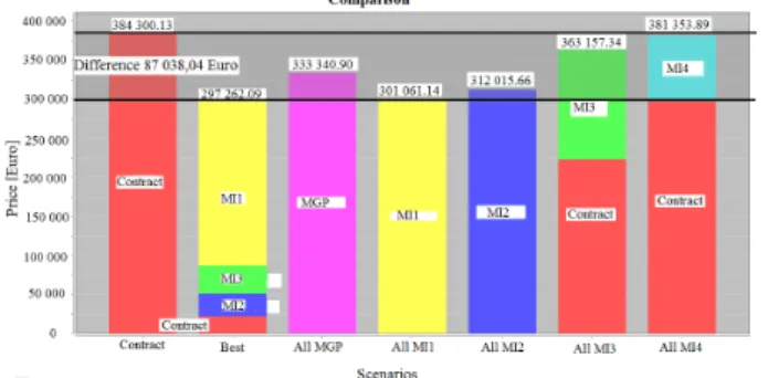
• on the third page the diagrams of the energetic consumption per market: contract, MI1, MI2, MI3, MI4, MGP (see Figure 10);
• on the fourth page, the cost of the kWh in function of the hour and of the market of purchase (see Figure 11).
Fig. 10. Composition of the markets for energy purchase.
Fig. 11. Price of the energy.
IV. RESULTS
The following Table I contains the consumptions in the first 4 days of the month of January. In the table are indicated the predicted consumption, the actual consumption and the error.
TABLEI CONSUMPTION AND ERRORS
Date Source Total 01/01/2013 Prediction [kWh] 774778.00
Consumption [kWh] 872159.20 Error [kWh] 97381.20 Error % 12.57 02/01/2013 Prediction [kWh] 3198944.40
Consumption [kWh] 2945989.20 Error [kWh] 535085 Error % 7.91 03/01/2013 Prediction [kWh] 4141000.00
Consumption [kWh] 3877623.20 Error [kWh] 517494.4 Error % 6.36 04/01/2013 Prediction [kWh] 42100000.00
Consumption [kWh] 3945766.00 Error [kWh] 449294.00 Error % 6.28
The plant average hourly consumption is 150 MWh, the average daily consumption is about 4000 MWh, whereas the total monthly consumption is 121484.8 MWh.
Figure 12 provides the valorization on the market. In the diagram are indicated the total cost for the effective consumption at the PUN (Unique National Price) of the last year (75.48 €/MWh), the cost for the effective consumption at the PUN hour by hour (as if all the purchases had been done on the MGP), the cost for the effective consumption at the real price suggested by the Sim Process system, the cost for the effective consumption at the best price of the 5 markets, the cost for the forecasted consumption.
Fig. 12. Valorization on the market.
In Table II is indicated the analysis ex post on the real consumptions for the month of January 2013.
With this analysis it is possible to calculate the savings obtained by a model of energy purchase based on purchases on the spot market according to the indications provided by the Sim Process system.
The saving is indicated as the difference of energy purchase at the hourly PUN in the MGP market, with respect to the purchase of the same energy amount on different markets (MGP, MI1, MI2, MI3, MI4) hour by hour suggested by the platform on the basis of the price forecasting in these markets.
The input of the analysis consists in the hourly consumptions of the plant [kWh] for a defined period of time. The consumptions are valorized in three different modalities: the first one is that considering the energy purchase at the hourly PUN price on the MGP. The second modality represents the energy purchases following the indications of the Sim Process system: are here employed the forecasted values calculated by the platform to find the cheapest market for each hourly purchase. Once found the market, the consumptions are valorized at the effective prices present on the database. The third modality is a benchmark, which is the price of purchase on the cheapest market looking at the results ex-post. It indicates how much the prediction platform can be improved. The output of this analysis consists in a table which shows the purchase price and the savings, and the performance with respect to the benchmark.
TABLEII RESULTS OF THE ANALYSIS
Total (Jan 2013) Euro Saving €/MWh Performance
PUN 7 822 448,00 64.39
Sim Process 7 421 645,00 61.09 - 53% Benchmark 6 961 931,00 57.31
The prices indicated are the pure purchase prices on the electric markets, net of system charges, network services and taxes.
V. CONCLUSIONS
The presented paper has described an integrated tool to provide a significant support to energy and plant managers in steel industry. Significant results were obtained from the real life application of the proposed methodologies. The obtained results are suitable for application in many other industrial cases where energy consumption plays a crucial role in the cost saving process.
REFERENCES
[1] E. Briano, C. Caballini, R. Revetria, A. Testa, M. De Leo, F. Belgrano, A. Bertolotto, Anticipation models for on-line control in steel industry: methodologies and case study, CP1303, Computing Anticipatory Systems, CASYS09 9th international conference.
[2] Ruey S. Tsay. Analysis of Financial Time Series. Wiley, 2005.. [3] J. E. Hanke, D. Wichern, A. G. Reitsch. Business Forecasting.
Prentice Hall, 2001, 7th edition.
[4] Peter J. Brockwell, Richard A. Davis. Time Series: Theory and Methods. Springer-Verlag, 1991.
[5] George E. P. Box, D. A. Pierce. Distribution of Residual Autocorrelations in Autoregressive-Integrated Moving Average Time Series Models. Journal of theAmerican Statistical Association, n° 65, pp. 1509–1526, 1970.
[6] G. M. Ljung, George E. P. Box. On a Measure of a Lack of Fit in Time Series Models. Biometrika, n° 65, pagg. 297–303, 1978. [7] E. F. Mendes, L. Oxley, M. Reale. Some new approaches to