www.atmos-chem-phys.net/11/9563/2011/ doi:10.5194/acp-11-9563-2011
© Author(s) 2011. CC Attribution 3.0 License.
Chemistry
and Physics
Re-analysis of tropospheric sulfate aerosol and ozone for the period
1980–2005 using the aerosol-chemistry-climate model
ECHAM5-HAMMOZ
L. Pozzoli1,*, G. Janssens-Maenhout1, T. Diehl2,3, I. Bey4, M. G. Schultz5, J. Feichter6, E. Vignati1, and F. Dentener1 1European Commission, Joint Research Centre, Institute for Environment and Sustainability, Ispra, Italy
2NASA Goddard Space Flight Center, Greenbelt, Maryland, USA 3University of Maryland Baltimore County, Baltimore, Maryland, USA
4Center for Climate Systems Modeling and Institute of Atmospheric and Climate Science, ETH Zurich, Zurich, Switzerland 5Forschungszentrum J¨ulich, Germany
6Max Planck Institute for Meteorology, Hamburg, Germany
*now at: Eurasia Institute of Earth Sciences, Istanbul Technical University, Turkey Received: 10 March 2011 – Published in Atmos. Chem. Phys. Discuss.: 30 March 2011 Revised: 12 August 2011 – Accepted: 29 August 2011 – Published: 16 September 2011
Abstract. Understanding historical trends of trace gas and aerosol distributions in the troposphere is essential to evalu-ate the efficiency of existing strevalu-ategies to reduce air pollution and to design more efficient future air quality and climate policies. We performed coupled photochemistry and aerosol microphysics simulations for the period 1980–2005 using the aerosol-chemistry-climate model ECHAM5-HAMMOZ, to assess our understanding of long-term changes and inter-annual variability of the chemical composition of the tro-posphere, and in particular of ozone and sulfate concentra-tions, for which long-term surface observations are avail-able. In order to separate the impact of the anthropogenic emissions and natural variability on atmospheric chemistry, we compare two model experiments, driven by the same ECMWF re-analysis data, but with varying and constant an-thropogenic emissions, respectively. Our model analysis in-dicates an increase of ca. 1 ppbv (0.055±0.002 ppbv yr−1) in global average surface O3 concentrations due to anthro-pogenic emissions, but this trend is largely masked by the larger O3anomalies due to the variability of meteorology and natural emissions. The changes in meteorology (not includ-ing stratospheric variations) and natural emissions account
Correspondence to:F. Dentener (frank.dentener@jrc.ec.europa.eu)
for the 75 % of the total variability of global average sur-face O3 concentrations. Regionally, annual mean surface O3 concentrations increased by 1.3 and 1.6 ppbv over Eu-rope and North America, respectively, despite the large an-thropogenic emission reductions between 1980 and 2005. A comparison of winter and summer O3 trends with mea-surements shows a qualitative agreement, except in North America, where our model erroneously computed a posi-tive trend. Simulated O3 increases of more than 4 ppbv in East Asia and 5 ppbv in South Asia can not be corroborated with long-term observations. Global average sulfate surface concentrations are largely controlled by anthropogenic emis-sions. Globally natural emissions are an important driver de-termining AOD variations. Regionally, AOD decreased by 28 % over Europe, while it increased by 19 % and 26 % in East and South Asia. The global radiative perturbation cal-culated in our model for the period 1980–2005 was rather small (0.05 W m−2for O
1 Introduction
Air quality is determined by the emission of primary pol-lutants into the atmosphere, by chemical production of sec-ondary pollutants and by meteorological conditions. The two air pollutants of most concern for public health, ozone (O3) and particulate matter (PM), have also strong impacts on climate. In the fourth Assessment Report of the Intergov-ernmental Panel on Climate Change (IPCC AR4), Solomon et al. (2007) estimate a Radiative Forcing (RF) from tropo-spheric ozone of +0.35 [−0.1, +0.3] W m−2, which corre-sponds to the third largest contribution to the total RF after carbon dioxide (CO2) and methane (CH4). IPCC AR4 also provides estimates for radiative forcing from aerosols. The direct RF (scattering and absorption of solar and infrared ra-diation) amounts to−0.5 [±0.4] W m−2, and the RF through indirect changes in cloud properties is estimated to−0.70 [−1.1,+0.4] W m−2.
Trends in global radiation and visibility measurements in-deed suggest an important role of aerosols. Solar radia-tion measurements showed a consistent and worldwide de-crease at the Earth’s surface (an effect dubbed “dimming”) from the 1960s. This trend reversed into “brightening” in the late 1990s in the US, Europe and parts of Korea (Wild, 2009). Similarly, an analysis of visibility measure-ments from 1973–2007 by Wang et al. (2009) suggests a global increase of AOD worldwide, except in Europe. Since, SO24−is one of the main aerosol components that determine the aerosol optical depth (Streets et al., 2009), the SO24− concentration reductions over Europe and US after the im-plementation of air quality policies may partly explain the dimming-brightening transition observed in the 1990s in Eu-rope, whereas in emerging economies such as China and India the emission of air pollutants rapidly increased since 1990.
Inter-annual meteorological variability in the last decades also strongly determined the variations of the concentrations and geographical distribution of air pollutants. For exam-ple, the El Ni˜no event in 1997–1998 and the period after the Mt. Pinatubo volcanic eruption in 1991 can explain much of the past chemical inter-annual variability of tropospheric O3, CH4and OH (Fiore et al., 2009; Dentener et al., 2003; Hess and Mahowald, 2009). In Europe, the infamous summer of 2003 led to a strong positive anomaly of solar surface radia-tion (Wild, 2009) and exacerbated ozone polluradia-tion at ground-level and throughout the troposphere (Solberg et al., 2008; Tressol et al., 2008).
Meteorological variability and changes in the precursor emissions of O3and SO24− are often concurrent processes, and their impact on surface concentrations is difficult to un-derstand from measurements alone (Vautard et al., 2006; Berglen et al., 2007). Therefore, there have been several efforts to re-analyze these trends using tropospheric chem-istry and transport models. For example, the European project REanalysis of the TROpospheric chemical
composi-tion (RETRO, Schultz et al., 2007) employed three different global models to simulate tropospheric ozone changes be-tween 1960 and 2000. Recently Hess and Mahowald (2009) analyzed the role of meteorology in inter-annual variability of tropospheric ozone chemistry.
In this paper, we extend these analyses by using a coupled aerosol-chemistry-climate simulation, and discuss our results in the light of the previous studies. We analyze the chemi-cal variability due to changes in meteorology (i.e. transport, chemistry) and natural emissions, and separate them from an-thropogenic emissions induced variability. The period 1980– 2005 was chosen because the advent of satellite observations in the 1970s introduced a discontinuity in the re-analysis of meteorological datasets (Hess and Mahowald, 2009; van Noije et al., 2006) and, as mentioned above, the considered period includes large meteorological anomalies. Particular attention will be given to four regions of the world (North America, Europe, East Asia, and South Asia) where signifi-cant changes in terms of the absolute amount of emitted trace gases and aerosol precursors occurred in the last decades. We will focus on past changes of O3and SO24−because of their importance for air quality and climate. Long measurement records are available since the 1980s and they will be used to evaluate our model results and the simulated trends. We further analyze changes in AOD, radiative perturbation (RP) and OH radical associated with changes in emissions and me-teorology.
The paper is organized as follows. In Sect. 2 the model description and experiment setup are outlined. In Sect. 3 an-thropogenic and natural emissions are described. Sections 4 and 5 present an analysis of global and regional variability and trends of O3and SO24−from 1980 to 2005. The regional analysis focuses on Europe (EU), North America (NA), East Asia (EA), and South Asia (SA) (Fig. 1, the region bound-aries were defined as in the HTAP study, Fiore et al., 2009). In Sect. 6 we will describe the anthropogenic radiative per-turbation due to changes in O3and SO24−. In Sects. 7 and 8 we will summarize the main findings and further discuss implications of our study for air quality-climate interactions.
2 Model and simulation descriptions
ECHAM5-Fig. 1. Map of the selected regions for the analysis and measurement stations with long records of O3and SO24−surface concentrations. North America (NA) [15◦N–55◦N; 60◦W–125◦W], Europe (EU) [25◦N–65◦N; 10◦W–50◦E], East Asia (EA) [15◦N–50◦N; 95◦E– 160◦E)], and South Asia (SA) [5◦N–35◦N; 50◦E–95◦E]. Triangles show the location of EMEP stations, squares of WDCGG stations, and diamonds of CASTNET stations. The stations are grouped in sub-regions: Northern Europe (NEU); Central Europe (CEU); Western Europe (WEU); Eastern Europe (EEU); Southern Europe (SEU); Western US (WUS): North-Eastern US (NEUS); Mid-Atlantic US (MAUS); Great lakes US (GLUS); Southern US (SUS).
HAMMOZ shares with many other global models and we refer for a further discussion to Ellingsen et al. (2008).
In this study a triangular truncation at wavenumber 42 (T42) resolution was used for the computation of the general circulation. Physical variables are computed on an associated Gaussian grid with a horizontal resolution of ca. 2.8◦×2.8◦ degrees. The model has 31 vertical levels from the surface up to 10 hPa and a time resolution for dynamics and chem-istry of 20 min. We simulated the period 1979–2005 (the first year is discarded from the analysis as spin-up). Me-teorology was taken from the ECMWF ERA-40 re-analysis (Uppala et al., 2005) until 2000 and from operational analy-ses (IFS cycle-32r2) for the remaining period (2001–2005). Even though we do not find any evidence for this we must note that this discontinuity may have an impact on the mete-orological variables and therefore on our analysis in the last years of the simulated period. Such discontinuities may also arise within a re-analysis data set due to the inclusion of dif-ferent data sets in the assimilation procedure. ECHAM5 vor-ticity, divergence, sea surface temperature, and surface pres-sure are relaxed towards the re-analysis data every time step with a relaxation time scale of 1 day for surface pressure and temperature, 2 days for divergence, and 6 h for vortic-ity (Jeuken et al., 1996). The relaxation technique forces the large scale dynamic state of the atmosphere as close as pos-sible to the re-analysis data, thus the model is in a consis-tent physical state at each time step but it calculates its own physics, e.g. for aerosols and clouds. The concentrations of CO2and other GHGs, used to calculate the radiative budget, were set according to the specifications given in Appendix II of the IPCC TAR report (Nakicenovic et al., 2000). In Ap-pendix A we provide a detailed description of the chemical and microphysical parameterizations included in ECHAM5-HAMMOZ. A detailed description of the ECHAM5 model can be found in Roeckner et al. (2003).
Two transient simulations were conducted:
– SREF: reference simulation for 1980–2005 where me-teorology and emissions are changing on an hourly-to-monthly basis;
– SFIX: simulation for 1980–2005 with anthropogenic emissions fixed at year 1980, while meteorology, nat-ural and wildfire emissions change as in SREF.
3 Emissions
3.1 Anthropogenic emissions
drivers as for BC and OC, and extended to the period 1980– 2006 (Streets et al., 2009) using annual fuel-use trends and economic growth parameters included in the IMAGE model (National Institute for Public Health and the Environment, 2001). Except for biomass burning, the BC, OC, and SO2 anthropogenic emissions were provided as annual averages. Primary emissions of SO24− are calculated as constant frac-tion (2.5 %) of the anthropogenic sulfur emissions. The SO2 and primary SO24− emissions from international ship traffic for the years 1970, 1980, 1995, and 2001, were based on the EDGAR 2000 FT inventory (van Aardenne et al., 2001) and linearly interpolated in time, using total emission estimates from Eyring et al. (2005a,b). The emissions of CO, NOx, and VOCs were available only until the year 2000. There-fore, we used for 2001–2005 the 2000 emissions, except for the regions where significant changes were expected between 2000 and 2005, such as US, Europe, East Asia and South East Asia (defined as in Fig. 1), for which derived emission trends of CO, NOx, and VOCs were applied to year 2000. The emission ratios between the period 2001–2005 and the year 2000 from the USEPA (http://www.epa.gov/ttn/chief/ trends/), EMEP (http://www.emep.int/), and REAS (http: //www.jamstec.go.jp/frcgc/research/p3/emission.htm) emis-sion inventories were applied to year 2000 emisemis-sions used for this study over the US, Europe, and Asia.
Table 1 summarizes the total annual anthropogenic emis-sions for the years 1980, 1985, 1990, 1995, 2000, and 2005. Global emissions of CO, VOCs and BC were relatively con-stant during the last decades, with small increases between 1980 and 1990, decreases in the 1990s and renewed increase between 2000 and 2005. During these 25 yr, global NOxand OC emissions increased up to 10 %, while sulfur emissions decreased by 10 %. However, these global numbers mask that the global distribution of the emission largely changed, with reductions over North America and Europe, balanced by strong increases in the economically emerging countries, such as China and India. Figure 2 shows the relative trends of anthropogenic emissions used during this study over the 4 se-lected world regions. In Europe and North America there is a general decrease of emissions of all pollutants from 1990 on. In East Asia and South Asia anthropogenic emissions gen-erally increase although for EA there is a decrease around 2000.
For the period 1980–2000, our global amounts of emission from anthropogenic sources, which are based on RETRO, are lower by more than 10 % for CO and NOx, and they are higher by more than 40 % for VOCs, when compared to the new emission inventory prepared by Lamarque et al. (2010) in support of the Intergovernmental Panel on Climate Change (IPCC) Fifth Assessment Report (AR5). For the pe-riod 2001–2005 several studies have recently shown signifi-cant changes in regional emissions, especially in Asia (e.g. Richter et al. (2005); Zhang et al. (2009); Klimont et al. (2009)). In our study, compared to the projection for year 2005 of Lamarque et al. (2010), which includes the
refer-Table 1. Global anthropogenic emissions of CO [Tg yr−1], NOx[Tg(N) yr−1], VOCs [Tg(C) yr−1], SO2[Tg(S) yr−1], SO42− [Tg(S) yr−1], OC [Tg yr−1], and BC [Tg yr−1].
1980 1985 1990 1995 2000 2005
CO 673.7 680.1 713.8 685.3 655.4 678.6
NOx 34.2 33.7 36.1 36.4 36.7 37.2
VOCs 84.6 85.0 87.9 84.8 80.5 84.3
SO2 67.1 67.2 66.2 61.0 58.8 59.0
SO42− 1.8 1.8 1.8 1.7 1.6 1.6
OC 7.8 8.2 8.3 8.7 8.5 8.7
BC 4.9 4.9 4.9 4.8 4.7 4.9
ences cited above, we applied: significantly lower emission reductions between 1980 and 2005 for CO and SO2in EU; larger reductions for BC and OC in both EU and NA; lower emission changes except for CO in EA; similar emission changes except for NOxand SO2in SA (Fig. 2).
3.2 Natural and biomass burning emissions
Some O3 and SO24− precursors are emitted by natural pro-cesses, which exhibit inter-annual variability due to chang-ing meteorological parameters (temperature, wind, solar ra-diation, clouds and precipitation). For example, VOC emis-sions from vegetation are influenced by surface temperature and short wavelength radiation, NOx is produced by light-ning and associated with convective activity, dimethyl sulfide (DMS) emissions depend on the phytoplankton blooms in the oceans and wind speed, and some aerosol species, such as mineral dust and sea salt, are strongly dependent on surface wind speed. Inter-annual variability of weather will therefore influence the concentrations of tropospheric O3 and SO24− and may also affect the radiative budget. The emissions from vegetation of CO and VOCs (isoprene and terpenes) were calculated interactively using the Model of Emissions of Gases and Aerosols from Nature (MEGAN) (Guenther et al., 2006). The total annual natural emissions in Tg(C) of CO and biogenic VOCs (BVOCs) for the period 1980– 2005 range from 840 to 960 Tg(C) yr−1with a standard de-viation of 26 Tg(C) yr−1(Fig. 3a), which corresponds to 3 % of the annual mean natural VOC emissions for the consid-ered period. 80 % of these total biogenic emissions occur in the tropics.
opposite trends over the same period (Schultz et al., 2007). An annual constant contribution of 9.3 Tg(N) yr−1 is in-cluded in our simulations for NOxemissions from microbial activity in soils (Schultz et al., 2007).
DMS, predominantly emitted from the oceans, is an SO24− aerosol precursor. Its emissions depend on seawater DMS concentrations associated with phytoplankton blooms (Ket-tle and Andreae, 2000) and model surface wind speed, which determines the DMS sea-air exchange (Nightingale et al., 2000). Terrestrial biogenic DMS emissions follow Pham et al. (1995). The total DMS emissions are ranging from 22.7 to 24.4 Tg(S) yr−1, with a standard deviation of 0.3 Tg(S) yr−1 or 1 % of annual mean emissions (Fig. 3c). The highest DMS emissions correspond to the 1997–1998 ENSO event. Since we have used a climatology of seawater DMS concentrations instead of annually varying concentra-tions, the variability may be misrepresented.
The emissions of sea salt are based on Schulz et al. (2004). The strong dependency on wind speed results in a range from 5000–5550 Tg yr−1 (Fig. 3e) with a standard deviation of 2 %.
Mineral dust emissions are calculated online using the ECHAM5 wind speed, hydrological parameters (e.g. soil moisture), and soil properties, following the work of Tegen et al. (2002) and Cheng et al. (2008). The total mineral dust emissions have a large inter-annual variability (Fig. 3d), ranging from 620 to 930 Tg yr−1, with a standard deviation of 72 Tg yr−1, almost 10 % of the annual mean average. Min-eral dust originating from the Sahara and over Asia con-tribute on average 58 % and 34 % to the global mineral dust emissions, respectively.
Biomass burning, from tropical savannah burning, de-forestation fires, and mid-and high latitude forest fires are largely linked to anthropogenic activities but fire severity (and hence emissions) are also controlled by meteorologi-cal factors such as temperature, precipitation and wind. We use the compilation of inter-annual varying biomass burning emissions published by Schultz et al. (2008), who used liter-ature data, satellite observations and a dynamical vegetation model in order to obtain continental-scale emission estimates and a geographical distribution of fire occurrence. We con-sider emissions of the components CO, NOx, BC, OC, and SO2, and apply a time-invariant vertical profile of the plume injection height for forest and savannah fire emissions. Fig-ure 3f shows the inter-annual variability for CO, NOx, and OC biomass burning emissions, with different peaks, such as in year 1998 during the strong ENSO episode.
Other natural emissions are kept constant during the en-tire simulation period. CO emissions from soil and ocean are based on the Global Emission Inventory Activity (GEIA) as in Horowitz et al. (2003), amounting to 160 and 20 Tg yr−1, respectively. Natural soil NOx emissions are taken from the ORCHIDEE model (Lathiere et al., 2006), resulting in 9 Tg(N) yr−1. SO
2volcanic emissions of 14 Tg(S) yr−1are from Andres and Kasgnoc (1998) and Halmer et al. (2002).
Since in the current model version secondary organic aerosol (SOA) formation is not calculated online, we applied a monthly varying OC emission (19 Tg yr−1) to take into ac-count the SOA production from biogenic monoterpenes (a factor of 0.15 is applied to monoterpene emissions of Guen-ther et al., 1995), as recommended in the AEROCOM project (Dentener et al., 2006).
4 Variability and trends of O3and OH during
1980–2005 and their relationship to meteorological variables
In this section we analyze the global and regional variability of O3and OH in relation to selected modeled chemical and meteorological variables. Section 4.1 will focus on global surface ozone, Sect. 4.2 will look into more detail to regional differences in O3, and for Europe and the US, compare the data to observations. Section 4.3 will describe the variabil-ity of the global ozone budget, and Sect. 4.4 will focus on the related changes in OH. As explained earlier, we will sep-arate the influence of meteorological and natural emission variability from anthropogenic emissions by differencing the SREF and SFIX simulations.
4.1 Global surface ozone and relation to meteorological variability
In Fig. 4 we show the ECHAM5-HAMMOZ SREF inter-annual monthly anomalies (difference between the monthly value and the 25-yr monthly average) of global mean surface temperature, water vapor, and surface concentrations of O3. SO24−, total column AOD and methane-weighted OH tropo-spheric concentrations will be discussed in later sections. To better visualize the inter-annual variability over 1980–2005, in Fig. 4, we also display the 12-months running average of monthly mean anomalies for both SREF (blue) and SFIX (red) simulations.
1980 1985 1990 1995 2000 2005
ï70
ï60
ï50
ï40
ï30
ï20
ï10 0
10 a) Anthropogenic emission changes over EU
%
CO:95.63 Tg yrï1 VOC:20.66 Tg(C) yrï1 NOx:7.53 Tg(N) yrï1 SO2:25.65 Tg(S) yrï1
BC:1.31 Tg yrï1
OC:1.63 Tg yrï1
1980 1985 1990 1995 2000 2005
ï60
ï50
ï40
ï30
ï20
ï10 0
10 b) Anthropogenic emission changes over NA
%
CO:127.40 Tg yrï1 VOC:26.11 Tg(C) yrï1 NOx:7.53 Tg(N) yrï1 SO2:12.89 Tg(S) yrï1
BC:0.68 Tg yrï1
OC:0.87 Tg yrï1
1980 1985 1990 1995 2000 2005
ï20 0 20 40 60 80 100 120 140
c) Anthropogenic emission changes over EA
%
CO:98.17 Tg yrï1
VOC:10.83 Tg(C) yrï1
NOx:2.96 Tg(N) yrï1
SO2:10.65 Tg(S) yrï1
BC:1.42 Tg yrï1
OC:1.94 Tg yrï1
19800 1985 1990 1995 2000 2005 50
100 150 200 250 300 350
d) Anthropogenic emission changes over SA
%
CO:60.15 Tg yrï1
VOC:5.53 Tg(C) yrï1
NOx:0.98 Tg(N) yrï1
SO2:1.47 Tg(S) yrï1
BC:0.39 Tg yrï1
OC:1.16 Tg yrï1
Fig. 2.Percentage changes in total anthropogenic emissions (CO, VOC, NOx, SO2, BC and OC) from 1980 to 2005 over the four selected
regions as shown in Fig. 1:(a)Europe, EU;(b)North America, NA;(c)East Asia, EA;(d)South Asia, SA. In the legend of each regional plot, the total annual emissions for each species are reported for the year 1980. The colored points represent the percentage changes in regional emissions between 1980 and 2005 in Lamarque et al. (2010) which includes recent assessments in the projections for the year 2005.
Fig. 3.Total annual natural and biomass burning emissions for the period 1980–2005:(a)biogenic CO and VOCs emissions from vegetation;
Table 2.Average, standard deviation (SD) and relative standard deviation (RSD, standard deviation divided by the mean) of globally averaged variables in this work for the simulation with changing anthropogenic emission and with fixed anthropogenic emissions (1980–2005). Three dimensional variables are density weighted and averaged between the surface and 280 hPa. Three dimensional quantities evaluated at the surface are prefixed with Sfc. The standard deviation is calculated as the standard deviation of the monthly anomalies (the monthly value minus the mean of all years for that month).
SREF SFIX
Average SD RSD Average SD RSD
Sfc O3(ppbv) 36.45 0.826 0.0227 35.97 0.627 0.0174
O3(ppbv) 48.37 1.1020 0.0228 47.64 0.8851 0.0186
CO (ppbv) 0.103 0.000416 0.0402 0.101 0.000529 0.0519
OH (molecules cm−3×10⁶) 1.20 0.016 0.013 1.18 0.029 0.024
HNO3(pptv) 129.11 14.70 0.1139 125.73 13.91 0.1106
Emi S (Tg yr−1) 104.2 3.49 0.0336 108.09 0.47 0.0043
SO2(pptv) 231.7 15.02 0.0648 246.9 8.70 0.0352
Sfc SO4−2(µg m−3) 1.12 0.071 0.0640 1.18 0.061 0.0515
SO4−2(µg m−3) 0.69 0.028 0.0406 0.72 0.025 0.0352
Fig. 5. Maps of surface O3concentrations and the changes due to anthropogenic emissions and natural variability. In the first column we show 5 yr averages (1981–1985) of surface O3concentrations over the selected regions, Europe, North America, East Asia, and South Asia. In the second column(b)we show the effect of anthropogenic emission changes in the period 2001–2005 on surface O3concentrations, calculated as the difference between SREF and SFIX simulations. In the third column(c)the natural variability of O3concentrations is shown, which is due to natural emissions and meteorology in the simulated 25 yr, calculated as the difference between the 5 yr average periods (2001–2005) and (1981–1985) in the SFIX simulation. The combined effect of anthropogenic emissions and natural variability is shown in column(d)and it is expressed as the difference between the 5 yr average period (2001–2005)–(1981–1985) in the SREF simulation.
The 25-yr global surface O3 average is 36.45 ppbv (Ta-ble 2) and increased by 0.48 ppbv compared to the SFIX simulation, with year 1980 constant anthropogenic emis-sions. About half of this increase is associated with anthro-pogenic emission changes (Fig. 4c (grey area)). The inter-annual monthly surface ozone concentrations varied by up to ±2.17 ppbv (1σ=0.83 ppbv), of which 75 % (0.63 ppbv in SFIX) was related to natural variations- especially the 1997– 1998 ENSO event.
4.2 Regional differences in surface ozone trends, variability, and comparison to measurements
Global trends and variability may mask contrasting regional trends. Therefore we also perform a regional analysis for North America (NA), Europe (EU), East Asia (EA) and South Asia (SA) (see Fig. 1). To quantify the impact on surface concentrations after 25 yr of changing anthropogenic emission, we compare the averages of two 5-yr periods, 1981–1985 and 2001–2005. We considered 5-yr averages to reduce the noise due to meteorological variability in these two periods.
In Fig. 5 we provide maps for the globe, Europe, North America, East Asia and South Asia (rows), showing in the first column (a) the reference surface concentrations, and in the other 3 columns relative to the period 1981–1985, the isolated effect of anthropogenic emission changes (b), mete-orological and natural emission changes (c), and combined changes (d). The global maps provide insight into inter-regional influences of concentrations.
Fig. 6. Trends of the observed (OBS) and calculated (SREF and SIFX) O3and SO24−seasonal anomalies (DJF and JJA) averaged over each group of stations as shown in Fig. 1: Northern Europe (NEU); Central Europe (CEU); Western Europe (WEU); Eastern Europe (EEU); Southern Europe (SEU); Western US (WUS): North-Eastern US (NEUS); Mid-Atlantic US (MAUS); Great lakes US (GLUS); Southern US (SUS). The vertical bars represent the 95 % confidence interval of the trends. The number of stations used to calculate the average seasonal anomalies for each subregion is shown in parentheses. Further details in Appendix B.
description of the data used for these summary figures, and their statistical comparison with model results.
We note here that O3and SO24−in ECHAM5-HAMMOZ were extensively evaluated in previous studies (Stier et al., 2005; Pozzoli et al., 2008a,b; Rast et al., 2011), showing in general a good agreement between calculated and observed SO24−and an overestimation of surface O3concentrations in some regions. We implicitly assume that this model bias does not influence the calculated variability and trends (Fig. B1 in Appendix B).
4.2.1 Europe
In Fig. 5e we show the SREF 1981–1985 annual mean EU surface O3(i.e. before large emission changes) correspond-ing to an EU average concentration of 46.9 ppbv. High an-nual average O3concentrations up to 70 ppbv are found over the Mediterranean basin, and lower concentrations between 20 to 40 ppbv in Central and Eastern Europe. Figure 5f shows the difference in mean O3concentrations between the SREF and SFIX simulation for the period 2001–2005. The de-cline of NOx and VOC anthropogenic emissions was 20 % and 25 %, respectively (Fig. 2a). Annual averaged surface O3concentration increases by 0.81 ppbv between 1981–1985 and 2001–2005. The spatial distribution of the calculated trends shows a strong variation over Europe: the computed O3increased between 1 and 5 ppbv over Northern and
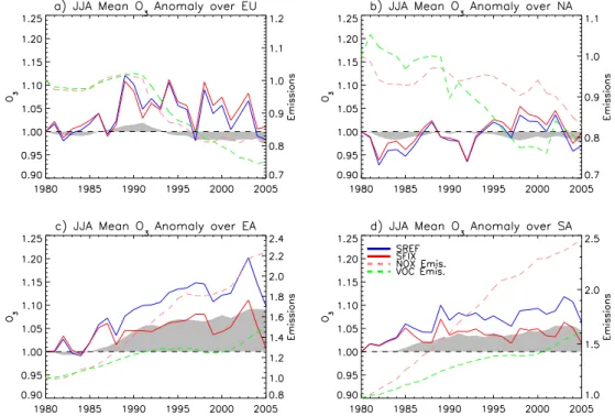
Fig. 7. Winter (DJF) anomalies of surface O3 concentrations averaged over the selected regions (shown in Fig. 1). On the left y-axis anomalies of O3surface concentrations for the period 1980–2005 are expressed as the ratios between seasonal means for each year and the year 1980. The blue line represents the SREF simulation (changing meteorology and changing anthropogenic emissions), the red line the SFIX simulation (changing meteorology and fixed anthropogenic emissions at the level of 1980), while the gray area indicates the SREF-SFIX difference. On the right y-axis the green and pink dashed lines represent the changes, i.e. the ratio between each year and 1980, of total annual VOC and NOxemissions, respectively.
caused upward trends in Northern and Central Europe, and downward trends in Southern Europe.
The regional responses of surface ozone can be compared to the HTAP multi-model emission perturbation study of Fiore et al. (2009), which considered identical regions and is thus directly comparable to this study. They found that the 20 % reduction over EU of all HTAP emissions deter-mined an increase of O3 by 0.2 ppbv in winter, and an O3 decrease by−1.7 ppbv in summer (average of 21 models), to a large extent driven by NOxemissions. Considering similar annual mean reductions in NOxand VOC emissions over Eu-rope from 1980–2005, we found a stronger emission driven increase of up to 3 ppbv in winter, and a decrease of up to 1 ppbv in summer. An important difference between the two studies may be the use of a spatially homogeneous emis-sion reduction in HTAP, while the emisemis-sions used here gener-ally included larger emission reductions in Northern Europe while emissions in Mediterranean countries remained more or less constant.
The calculated and observed O3 trends for the period 1990–2005 are relatively small compared to the inter-annual variability. In winter (DJF) (Fig. 6) measured trends con-firm increasing ozone in most parts of Europe. The observed trends are substantially larger (0.3–0.5 ppbv yr−1) than the model results (0–0.2 ppbv yr−1), except in Western Europe (WEU). In summer (JJA) the agreement of calculated and observed trends is small: in the observations they are close to zero for all European regions with large 95 % confidence intervals, while calculated trends show significant decreases (0.1–0.45 ppbv yr−1) of O
3. Despite seasonal O3trends not being well captured by the model, the seasonally averaged modeled and measured surface ozone concentrations are rea-sonably well correlated for a large number of stations (Ap-pendix B). In winter the simulated inter-annual variability seemed to be somewhat underestimated, pointing to miss-ing variability commiss-ing from e.g. stratosphere-troposphere or long-range transport. In summer the correlations are gener-ally increasing for Central Europe and decreasing for West-ern Europe.
Our results are generally in good agreement with previous estimates of observed O3 trends, e.g. Jonson et al. (2006); Lamarque et al. (2010); Cui et al. (2011); Wilson et al. (2011). In those studies they reported observed annual O3 trends of 0.32–0.40 ppbv yr−1for stations in central Europe, which are comparable with the observed trends calculated in our study (Fig. B3 in Appendix B). In Mace Head Lamar-que (2010) reported an increasing trend of 0.18 ppbv yr−1, comparable to our study (Fig. B3 in Appendix B). Jonson et al. (2006) reported seasonal trends of O3ranging between 0.13 and 0.5 ppbv yr−1 in winter (JF) and between −0.59 and−0.12 ppbv yr−1in summer (JJA). Wilson et al. (2011) calculated positive annual O3 trends in Central and North-Western Europe (0.14–0.41 pbbv yr−1), and significant nega-tive annual trends at 11 % of sites mainly located in Eastern and South-Western Europe (−1.28–−0.24 pbbv yr−1).
4.2.2 North America
Computed annual mean surface O3 over North America (Fig. 5i) for 1981–1985 was 48.3 ppbv. Higher O3 concentra-tions are found over California and in the continental outflow regions, Atlantic and Pacific Oceans, and the Gulf of Mex-ico, and lower concentrations north of 45◦N. Anthropogenic NOxin NA decreased by 17 % between 1980 and 2005, par-ticularly in the 1990s (−22 %) (Fig. 2b). These emission reductions produced an annual mean O3 concentration de-crease up to 1 ppbv over all the Eastern US, 1–2 ppbv over the Southern US, and 1 ppbv in the Western US. Changes in anthropogenic emissions from 1980 to 2005 (Fig. 5j) re-sulted in a small average increase of ozone by 0.28 ppbv over NA, where effects on O3of emission reductions in the US and Canada were balanced by higher O3concentrations mainly over the tropics (below 25◦N). Changes in
meteorol-ogy and natural emissions (Fig. 5k) increased O3 between 1 and 5 ppbv over the continent, and reduced O3 by up to 5 ppbv over Western Mexico and the Atlantic Ocean (aver-age of 0.89 ppbv over the entire region). Thus natural vari-ability was the largest driver of the over-all average regional increase of 1.58 ppbv in SREF (Fig. 5l). Over NA natu-ral variability is the main driver of summer (JJA) O3 fluc-tuations from −7 % to 5 % (Fig. 8b). In winter (Fig. 7b), the contribution of emissions and chemistry is strongly in-fluencing these relative changes. Computed and measured summer concentrations were better correlated than those in winter (Appendix B). However, while in winter, an analy-sis of the observed trends seems to suggest 0–0.2 ppbv yr−1 O3increases, the model predicts small O3decreases instead, though these differences are not often significant (see also Appendix B). In summer modeled upward trends (SREF) are not confirmed by measurements, except for the Western US (WUS). These computed upward trends were strongly deter-mined by the large-scale meteorological variability (SFIX), and the model trends solely based on anthropogenic emis-sion changes (SREF-SFIX) would be more consistent with observations.
Despite the difficulty in comparing trends calculated with different methods and for different periods, our observed trends are qualitatively in good agreement with previous studies over the Western US: Oltmans et al. (2008) observed positive trends at some sites, but no significant changes at others; Jaffe and Ray (2007) estimated positive O3 trends of 0.21–0.62 ppbv yr−1in winter and 0.43–0.50 ppbv yr−1in summer; Parrish et al. (2009) found 0.43±0.17 ppbv yr−1 in winter and 0.24±0.16 ppbv yr−1 in summer O
4.2.3 East Asia
In East Asia, we calculated an annual mean surface O3 con-centration of 43.6 ppbv for 1981–1985. Surface O3is less than 30 ppbv over North-Eastern China, and influenced by continental outflow conditions, up to 50 ppbv concentrations are computed over the Northern Pacific Ocean and Japan (Fig. 5m). Over EA, anthropogenic NOxand VOC emissions increased by 125 % and 50 %, respectively, from 1980 to 2005. Between 1981–1985 and 2001–2005 O3is reduced by 10 ppbv in North Eastern China, due to reaction with freshly emitted NO. In contrast, O3concentrations increase close to the coast of China by up to 10 ppbv, and up to 5 ppbv over the entire north Pacific, reaching North America (Fig. 5b). For the entire EA region (Fig. 5n) we found an increase of annual mean O3concentrations of 2.43 ppbv. The effect of meteo-rology and natural emissions is generally significantly posi-tive, with an EA-wide increase of 1.6 ppbv, and up to 5 ppbv in northern and southern continental EA (Fig. 5o). The com-bined effect of anthropogenic emissions and meteorology is an increase of 4.13 ppbv in O3concentrations (Fig. 5p). Dur-ing this period, the seasonal mean O3concentrations were increasing by 3 % and 9 % in winter and summer, respec-tively (Figs. 7c and 8c). The effect of natural variability on the seasonal mean O3concentrations shows opposite effects in winter and summer: a reduction between 0 and 5 % in win-ter, and an increase between 0 and 10 % in summer. The 3 long-term measurement datasets at our disposal (not shown) indicate large inter-annual variability of O3 and no signifi-cant trend in the time period from 1990 to 2005, therefore they are not plotted in Fig. 6.
4.2.4 South Asia
Of all 4 regions, the largest relative change in anthropogenic emissions occurred over SA: NOx emissions increased by 150 %, VOC by 60 %, and sulfur by 220 %. South Asian O3inter-annual variability is rather different from EA, NA, and EU, because the SA region is almost completely situ-ated in the tropics. Meteorology is highly influenced by the Asian monsoon circulation, with the wet season in June– August. We calculate an annual mean surface O3 concen-tration of 48.2 ppbv, with values between 45 and 60 ppbv over the continent (Fig. 5q). Note that the high concentra-tions at the northern edge of the region may be influenced by the orography of the Himalaya. The increasing anthro-pogenic emissions enhanced annual mean surface O3 con-centrations by on average 4.24 ppbv (Fig. 5r), and more than 5 ppbv over India and the Gulf of Bengal. In the NH winter (dry season) the increase in O3concentrations of up to 10 % due to anthropogenic emissions is more pronounced than in the summer (wet season), with an increase of only 5 % in JJA (Figs. 7d and 8d). The effect of meteorology produced an an-nual mean O3increase of 1.15 ppbv over the region and more than 2 ppbv in the Ganges valley and in the southern Gulf of
Bengal (Fig. 5s). The total variability in seasonal mean O3 concentrations is on the order of 5 %, both in winter and sum-mer (Figs. 7d and 8d). In 25 yr, the computed annual mean O3concentrations increased by 5.12 ppbv over SA, approxi-mately 75 % of which are related to increasing anthropogenic emissions (Fig. 5t). Unfortunately, to our knowledge no such long-term data of sufficient quality exist in India.
4.3 Variability of the global ozone budget
We will now discuss the changes in global tropospheric O3. To put our model results in a multi-model context, we show in Fig. 9 the global tropospheric O3budget along with budget terms derived from Stevenson et al. (2006). O3budget terms were calculated using an assumed chemical tropopause, with a threshold of 150 ppbv of O3. The annual globally integrated chemical production (P), loss (L), surface deposition (D), and stratospheric influx (Sinf=L+D−P) terms are well in the range of those reported by Stevenson et al. (2006), though O3burden and lifetime are at the high end. In our study, the variability in production and loss are clearly determined by meteorological variability, with the 1997–1998 ENSO event standing out. The increasing turnover of tropospheric ozone manifests in gradually decreasing ozone lifetimes (−1 day from 1980 to 2005), while total tropospheric ozone burden increases from 370 to 380 Tg, caused by increasing produc-tion and stratospheric influx.
Further, we compare our work to a re-analysis study by Hess and Mahowald (2009), which focused on the relation-ship between meteorological variability and ozone. Hess and Mahowald (2009) used the chemical transport model (CTM) MOZART2 to conduct two ozone simulations from 1979 to 1999 without considering the inter-annual changes in emis-sions (except for lightning emisemis-sions) and is thus very com-parable to our SFIX simulation. The simulations were driven by two different re-analysis methodologies: the National Center for Environmental Prediction/National Center for At-mospheric Research (NCEP/NCAR) re-analysis; the output of the Community Atmosphere Model (CAM3, Collins et al., 2006), driven by observed sea surface temperatures (SNCEP and SCAM in Hess and Mahowald (2009), respectively). The comparison of our model (in particular the SFIX simulation) driven by the ECMWF ERA-40 re-analysis with Hess and Mahowald (2009) provides insight in the extent to which these different approaches impact the inter-annual variabil-ity of ozone. In Table 3 we compare the results of SFIX with the two Hess and Mahowald (2009) model results. We ex-cluded the last 5 yr of our SFIX simulation in order to allow direct statistical comparison with the period 1980–2000.
4.3.1 Hydrological cycle and lightning
The variability of photolysis frequencies of NO2 (JNO2) at
Table 3. Average, standard deviation (SD) and relative standard deviation (RSD, standard deviation divided by the mean) of globally averaged variables in this work, SCAM and SNCEP(Hess and Mahowald, 2009) (1980–2000). Three dimensional variables are density weighted and averaged between the surface and 280 hPa. Three dimensional quantities evaluated at the surface are prefixed with Sfc. The standard deviation is calculated as the standard deviation of the monthly anomalies (the monthly value minus the mean of all years for that month).
ERA-40 (this work SFIX) SCAM (Hess, 2009) SNCEP (Hess, 2009)
Average SD RSD Average SD RSD Average SD RSD
SfcT (K) 287 0.112 0.000391 287 0.116 0.000403 287 0.121 0.00042
SfcJNO2(s−1×10⁻³) 2.13 0.0121 0.00567 2.43 0.00454 0.00187 2.39 0.00814 0.00341
LNO (TgN yr−1) 3.91 0.153 0.0387 4.71 0.118 0.0251 2.79 0.211 0.0759
PRECT (mm day−1) 2.95 0.0331 0.011 2.42 0.0145 0.006 2.4 0.0389 0.0162
Q(g kg−1) 4.72 0.060 0.0127 3.46 0.0411 0.0119 3.38 0.0361 0.0107
O3(ppbv) 47.79 0.819 0.01714 46 0.192 0.00418 48.4 0.752 0.0155
Sfc O3(ppbv) 36.1 0.595 0.0165 29.8 0.122 0.0041 31.2 0.468 0.015
CO (ppbv) 0.100 0.000450 0.04482 0.083 0.000449 0.00542 0.0847 0.000388 0.00458
OH (mole mole−1×10¹⁵) 63.1 1.269 0.02012 73.5 0.707 0.00962 70.4 0.847 0.012
HNO3(pptv) 127 13.95 0.1096 121 1.22 0.0101 121 1.49 0.0123
Fig. 9. Global tropospheric O3 budget calculated for the period 1980–2005 for the SREF (blue) and SFIX (red) ECHAM5-HAMMOZ simulations:(a)chemical production (P);(b)chemical loss (L);(c)surface deposition (D);(d)stratospheric influx (Sinf=L+D−P);(e)
tropospheric burden (BO3);(f)lifetime (τO3=BO3/(L+D)). The black points for the year 2000 represent the mean±standard deviation budgets as found in the multi model study of Stevenson et al. (2006).
JNO2values are ca. 10 % lower in our SFIX (ECHAM5)
sim-ulation compared to the two simsim-ulations reported by Hess and Mahowald (2009). This may be due to a different rep-resentation of the cloud impact on photolysis frequencies (in presence of a cloud layer lower rates at surface and higher rates above) as calculated in our model using Fast-J.2 (see
processes involving the hydrological cycle, especially in the NH summer in the tropics. The computed production of NOx from lightning (LNO) of 3.91 Tg yr−1 in our SFIX simu-lation resides between the values found in the NCEP- and CAM-driven simulations of Hess and Mahowald (2009), de-spite the large uncertainties of lightning parameterizations (see Sect. 3.2).
4.3.2 Variability, re-analysis and nudging methods
The global multi annual averages of the meteorological vari-ables and gas concentrations at the surface and in the tropo-sphere are rather similar in the 3 simulations (Table 3). O3is ranging from 46 to 48.4 ppbv, while 20 % higher values are found for surface O3in our SFIX simulation. Our global tro-pospheric average of CO concentrations is 15 % higher than in Hess and Mahowald (2009), probably due to different bio-genic CO and VOCs emissions. Despite larger amounts of water vapor, and lower surface JNO2 in SFIX, our calcu-lated OH tropospheric concentrations are smaller by 15 %. Remarkable differences compared to Hess and Mahowald (2009) are found in the inter-annual variability. In general the variability calculated in our SFIX simulation is closer to the SNCEP simulation of Hess and Mahowald (2009), but our model exhibits a larger inter-annual variability of global O3, CO, OH, and HNO3 than the CAM-driven simulation analysis by Hess and Mahowald (2009). This likely indi-cates that nudging with different re-analysis datasets (such as ECMWF and NCEP), or only prescribing monthly averaged sea-surface temperatures, can give significantly different an-swers on the processes that govern inter-annual variations in the chemical composition of the troposphere. The variability of OH (calculated as the relative standard deviation, RSD) in our SFIX simulation is higher by a factor of 2 than those in SCAM and SNCEP, and CO, HNO3up to a factor of 10. We speculate that these differences point to differences in the hydrological cycle among the models, which influence OH through changes in cloud cover and HNO3through different washout rates. A similar conclusion was reached by Auvray et al. (2007), who analyzed ozone formation and loss rates from the ECHAM5-MOZ and GEOS-CHEM models for dif-ferent pollution conditions over the Atlantic Ocean. Since the methodology used in our SFIX simulation should be rather comparable to that used for the NCEP-driven MOZART2 simulation, we speculate that in addition to the differences in re-analysis (NCEP/NCAR and ECMWF/ERA-40), also dif-ferent nudging methodologies may strongly impact the cal-culated inter-annual variabilities.
4.4 OH variability
The main processes that contribute to the OH variabil-ity are both meteorological and chemical. Dentener et al. (2003) found that OH variability for the period 1979–1993 was mainly driven by meteorological processes, i.e.
However, we do not want to over-interpret this decline, since in this period we used meteorological data from the opera-tional ECMWF analysis instead of ERA-40 (Sect. 2). On the other hand we have no evidence of other discontinuities in our analysis, and the magnitude of the OH changes was similar to earlier changes in the period 1980–1995.
5 Surface and column SO24−
In this section we analyze global and regional sulfate sur-face concentrations (Sect. 5.1) and the global sulfate budget (Sect. 5.2) including their variability. The regional analysis and comparison with measurements follows the approach of the ozone analysis above.
5.1 Global and regional surface sulfate
Global average surface SO24− concentrations are 1.12 and 1.18 µg(S) m−3 for the SREF and SFIX runs, respectively (Table 2). Anthropogenic emission changes induce a de-crease of ca. 0.1 µg(S) m−3SO24−between 1980 and 2005 in SREF (Fig. 4e). Monthly anomalies of SO24−surface concen-trations range from−0.1, to 0.2 µg(S) m−3. The 12-month running averages of monthly anomalies are in the range of ±0.1 µg(S) m−3for SREF, and about half of this in the SFIX simulation. The anomalies in global average SO24−surface concentrations do not show a significant correlation with me-teorological variables on the global scale.
5.1.1 Europe
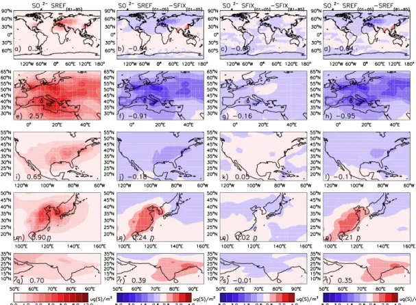
For 1981–1985 we compute an annual average SO24−surface concentration of 2.57 µg(S) m−3(Fig. 10e), with the largest values over the Mediterranean and Eastern Europe. Emis-sion controls (Fig. 2a) reduced SO24−surface concentrations (Figs. 10f, 11a, and 12a) by almost 50 % in 2001–2005. Fig-ures 10f and g show that emission reductions and meteoro-logical variability contribute ca. 85 % and 15 % respectively, to the overall differences between 2001–2005 and 1981– 1985, indicating a small but significant role for meteorolog-ical variability in the SO24− signal. Figure 10h shows that the largest SO24−decreases occurred in Southern and North-Eastern Europe. In Figs. 11a and 12a we display seasonal differences in the SO24−response to emissions and meteoro-logical changes. SFIX European winter (DJF) surface sulfate varies±30 % compared to 1980, while in summer (JJA) con-centrations are between 0 and 20 % larger than in 1980. The decline of European surface sulfur concentrations in SREF is larger in winter (50 %) than in summer (37 %).
Measurements mostly confirm these model findings. In-deed, inter-annual seasonal anomalies of SO24− in winter (Appendix B) generally correlate well (R >0.5) at most sta-tions in Europe. In summer, the modeled inter-annual vari-ability is always underestimated (normalized standard
devi-ation of 0.3–0.9), most likely indicating an underestimate in the variability of precipitation scavenging in the model over Europe. Modeled and measured SO24− trends are in good agreement in most European regions (Fig. 6). In winter the observed declines of 0.02–0.07 µg(S) m−3yr−1 are un-derestimated in NEU and EEU, and overestimated in the other regions. In summer the observed declines of 0.02– 0.08 µg(S) m−3yr−1 are overestimated in SEU, and under-estimated in CEU, WEU, and EEU.
5.1.2 North America
The calculated annual mean surface concentration of sul-fate over the NA region for the period 1981–1985 is 0.65 µg(S) m−3. Highest concentrations are found over the Eastern and Southern US (Fig. 10i). NA emissions reduc-tions of 35 % (Fig. 2b) reduced SO24−concentrations on av-erage by 0.18 µg(S) m−3), and up to 1 µg(S) m−3 over the Eastern US (Fig. 10j). Meteorological variability results in a small overall increase of 0.05 µg(S) m−3(Fig. 10k). Changes in emissions and meteorology can almost be combined lin-early (Fig. 10l). The total decline is thus 0.11 µg(S) m−3: −20 % in winter and−25 % in summer between 1980–2005, indicating a fairly low seasonal dependency.
Like in Europe, also in North America measured inter-annual seasonal variability is smaller than in our calcu-lations in winter and larger in summer (Appendix B). Observed winter downward trends are in the range of 0–0.03 µg(S) m−3yr−1 in reasonable agreement with the range of 0.01–0.06 µg(S) m−3yr−1 calculated in the SREF simulation. In summer, except for the Western US (WUS), observed SO24− trends range between −0.08 and −0.05 µg(S) m−3yr−1, and the calculated trends decline only between 0.03–0.04 µg(S) m−3yr−1) (Fig. 6). We suspect that a poor representation of the seasonality of anthropogenic sul-fur emissions contributes to both the winter overestimate and the summer underestimate of the SO24−trends.
5.1.3 East Asia
Fig. 10.As Fig. 5 but for SO24−surface concentrations.
5.1.4 South Asia
Annual and regional average SO24− surface concentrations of 0.70 µg(S) m−3 (1981–1985) increased by on average 0.39 µg(S) m−3, and up to 1 µg(S) m−3over India, due to the 220 % increase in anthropogenic sulfur emissions in 25 yr. The alternation of wet and dry seasons is greatly influencing the seasonal SO24−concentration changes. In winter (dry sea-son), following the emissions, the SO24− concentrations in-crease two-fold. In the wet season (JJA) we do not see a sig-nificant increase in SO24−concentrations and the variability is almost completely dominated by the meteorology (Figs. 11d and 12d). This indicates that frequent rainfall in the monsoon circulation keeps SO24− low regardless of increasing emis-sions. In winter we calculated a ratio of 0.45 between SO24− wet deposition and total SO24−production (both gas and liq-uid phases), while during summer months about 1.24 times more sulfur is deposited in the SA region than is produced.
5.2 Variability of the global SO24−budget
We now analyze in more detail the processes that contribute to the variability of surface and column sulfate. Figure 13 shows that inter-annual variability of the global SO24−burden is largely determined by meteorology in contrast to the
Fig. 11. Winter (DJF) anomalies of surface SO24−concentrations averaged over the selected regions (shown in Fig. 1). On the left y-axis anomalies of SO24−surface concentrations for the period 1980–2005 are expressed as the ratios between seasonal means for each year and the year 1980. The blue line represents the SREF simulation (changing meteorology and changing anthropogenic emissions), the red line the SFIX simulation (changing meteorology and fixed anthropogenic emissions at the level of 1980), while the gray area indicates the SREF-SFIX difference. On the right y-axis the pink dashed line represents the changes, i.e. the ratio between each year and 1980, of total annual sulfur emissions.
Fig. 13.Global tropospheric SO24−budget calculated for the period 1980–2005 for the SREF (blue) and SFIX (red) ECHAM5-HAMMOZ simulations:(a)total sulfur emissions;(b)SO24−liquid phase production;(c)SO24−gaseous phase production;(d)surface deposition;(e)
SO24−burden;(f)lifetime.
6 Variability of AOD and anthropogenic radiative perturbation of aerosol and O3
The global annual average total aerosol optical depth (AOD) ranges between 0.151 and 0.167 during the period 1980– 2005 (SREF), which is slightly higher than the range of model/measurement values (0.127–0.151) reported by Kinne et al. (2006). The monthly mean anomalies of total AOD (Fig. 4f, 1σ=0.007 or 4.3 %) are determined by variations of natural aerosol emissions, including biomass burning; the changes in anthropogenic SO2 emissions discussed above only cause little differences in global AOD anomalies. The effect of anthropogenic emissions is more evident at the re-gional scale. Figure 14a shows the AOD 5-yr average cal-culated for the period 1981–1985, with a global average of 0.155. The changes in anthropogenic emissions (Fig. 14b) decrease AOD over a large part of the Northern Hemisphere, in particular over Eastern Europe, and they largely increase AOD over East and South Asia. The effect of meteorology and natural emissions is smaller, ranging between−0.05 and 0.1 (Fig. 14c), and it is almost linearly adding to the effect of anthropogenic emissions (Fig. 14d).
In Fig. 15 and Table 5 we see that over EU the reduc-tions in anthropogenic emissions produced a 28 % decrease in AOD, and 14 % over NA. In EA and SA the increasing emissions, and particularly sulfur emissions, produced an
in-Table 4. Relationships, in Tg(S) per Tg(S) emitted, calculated for the period 1980–2005 between sulfur emissions and SO24−burden
(B), SO24−production from SO2in-cloud oxidation (In-cloud), and SO24−gaseous phase production (Cond) over Europe (EU), North America (NA), East Asia (EA), and South Asia (SA).
EU NA EA SA
slope R2 slope R2 slope R2 slope R2
B (×10−3) 2.21 0.86 0.79 0.12 2.86 0.79 5.36 0.90 In-cloud 0.31 0.97 0.38 0.93 0.25 0.79 0.18 0.90 Cond 0.08 0.93 0.09 0.70 0.17 0.85 0.37 0.98
crease of AOD of 19 % and 26 %, respectively. The variabil-ity in AOD due to natural aerosol emissions and meteorology is significant. In SFIX the natural variability of AOD is up to 10 % over EU, 17 % over NA, 8 % over EA, and 13 % over SA. Interestingly, over NA the resulting AOD in the SREF simulation does not show a large signal. The same re-sults were qualitatively found also from satellite observations (Wang et al., 2009), where the AOD decreased only over Eu-rope, no significant trend was found for North America, and it increased in Asia.
Table 5.Globally and regionally (EU, NA, EA, and SA) averaged effect of changing anthropogenic emissions (SREF-SFIX) during the 5-yr periods 1981–1985 and 2001–2005 on: surface concentrations of O3(ppbv), SO24−(%), and BC (%); total aerosol optical depth (AOD) (%) and total column O3(DU); the total anthropogenic aerosol radiative perturbation at top of the atmosphere (RPTOAaer ), at surface (RPSURFaer ) (W m−2), and in the atmosphere (RPATMaer =(RPTOAaer −RPSURFaer ); the anthropogenic radiative perturbation of O3(RPO3); correlations calcu-lated over the entire period 1980–2005 between anthropogenic RPTOAaer and1AOD; between anthropogenic RPSURFaer and1AOD; between
RPATMaer and1AOD; between RPATMaer and1BC; between anthropogenic RPO3 and1O3at surface; between anthropogenic RPO3 and1O3
column. High correlation coefficients are highlighted in bold.
GLOBAL EU NA EA SA
1O3[ppb] 0.98 0.81 0.27 2.44 4.25
1SO24−[%] −10 −36 −25 27 59
1BC [%] 0 −43 −34 30 70
1AOD [%] 0 −28 −14 19 26
1O3[DU] 1.18 1.35 1.54 2.85 2.99
RPTOAaer [W m−2] 0.02 1.26 0.39 −0.53 −0.54
RPSURFaer [W m−2] −0.03 2.05 0.71 −1.19 −1.83
RPATMaer [W m−2] 0.05 −0.79 −0.32 0.66 1.29
RPO3[W m−2] 0.05 0.05 0.06 0.12 0.15
slope R2 slope R2 slope R2 slope R2 slope R2
RPTOAaer [W m−2] vs.1AOD −17.86 0.85 −16.1 0.99 −16.99 0.97 −13.57 0.99 −13.84 0.99
RPSURFaer [W m−2] vs.1AOD −1.32 0.24 −26.71 0.99 −28.10 0.97 −28.95 0.99 −47.57 0.99
RPATMaer [W m−2] vs.1AOD −4.62 0.03 10.61 0.93 11.11 0.68 15.38 0.97 33.73 0.98
RPATMaer [W m−2] vs.1BC [ %] 0.35 0.11 1.73 0.99 0.95 0.99 1.92 0.97 1.74 0.99
RPO3[mW m−2] vs.1O3[ppbv] 42.8 0.91 35.2 0.65 51.3 0.49 46.7 0.94 36.0 0.97
RPO3[mW m−2] vs.1O3[DU] 40.8 0.99 36.4 0.99 44.2 0.99 44.1 0.99 49.1 0.99
1981–1985 and 2001–2005. We define the difference be-tween the instantaneous clear-sky total aerosol and all sky O3 RF of the SREF and SFIX simulations, as the total aerosol and O3short-wave radiative perturbation due to an-thropogenic emissions, and we will refer to them as RPaer and RPO3, respectively.
6.1 Aerosol radiative perturbation
The instantaneous aerosol radiative forcing (RF) in ECHAM5-HAMMOZ is diagnostically calculated from the difference in the net radiative fluxes including and excluding aerosol (Stier et al., 2007). For aerosol we focus on clear sky radiative forcing, since unfortunately a coding error pre-vents us from evaluating all-sky forcing. In Fig. 15 we show, together with the AOD (see before), the evolution of the nor-malized RPaer, at the top-of-the-atmosphere (RPTOAaer ) and at the surface (and RPSurfaer ).
For Europe, the AOD change by−28 % (mainly due to changes in removal of SO24−aerosol) leads to an increase of RPTOAaer of 1.26 W m−2and RPSurfaer of 2.05. The 14 % AOD reduction in NA corresponds to a RPTOAaer of 0.39 W m−2and RPSurfaer of 0.71 W m−2. In EA and SA, AOD increased by 19 % and 26 %, corresponding to a RPTOAaer of −0.53 and −0.54 W m−2, respectively, while at surface we found RP
aer of −1.19 W m−2 and−1.83 W m−2. The larger difference
between TOA and surface forcing in South Asia compared to the other regions indicates a much larger contribution of BC absorption in South Asia.
Globally, we found a significant correlation between the anthropogenic aerosol radiative perturbation at the top of the atmosphere with the percentage changes in AOD due to an-thropogenic emissions (Table 5, R2=0.85 for RPTOAaer vs. 1AOD), while there is no correlation between anthropogenic aerosol radiative perturbation and anthropogenic changes in AOD (1AOD) or BC (1BC) at the surface and in the at-mosphere. Within the four selected regions the correlation between anthropogenic emission induced changes in AOD and RPaer at the top-of-the-atmosphere, surface and the at-mosphere is much higher (R2>0.93 for all regions except for RPATMaer over NA; Table 5).
We calculate a relatively constant RPTOAaer between−17 to −13 W m−2 per unit AOD around the world; and a larger range of−48 to−26 W m−2per unit AOD for RP
Fig. 14.Maps of total aerosol optical depth (AOD) and the changes due to anthropogenic emissions and natural variability. We show(a)the 5-yr averages (1981–1985) of global AOD;(b)the effect of anthropogenic emission changes in the period 2001–2005 on AOD, calculated as the difference between SREF and SFIX simulations;(c)the natural variability of AOD, which is due to natural emissions and meteorology in the simulated 25 yr, calculated as the difference between the 5-yr average periods (2001–2005) and (1981–1985) in the SFIX simulation;
(d)the combined effect of anthropogenic emissions and natural variability expressed as the difference between the 5-yr average period (2001–2005)–(1981–1985) in the SREF simulation.
6.2 Ozone radiative perturbation
For convenience and completeness, we also present in this section a calculation of O3 RP diagnosed using ECHAM5-HAMMOZ O3 columns, in combination with all-sky radia-tive forcing efficiencies provided by D. Stevenson (personal communication, 2008; for a further discussion, Gauss et al., 2006). Table 5 and Fig. 5 show that O3total column and sur-face concentrations increased by 1.54 DU (1.58 ppbv) over NA, 1.35 DU (1.28 ppbv) over EU, 2.85 (4.13 ppbv) over EA, and 2.99 DU (5.12 ppbv) over SA in the period 1980– 2005. The RPO3 over the different regions reflect the total
column O3changes, 0.05 W m−2over EU, 0.06 W m−2over NA, 0.12 W m−2over EA, and 0.15 W m−2over SA. As ex-pected, the spatial correlation of O3 columns and radiative perturbations is nearly 1, also the surface O3concentrations in EA and SA correlate nearly as well with the radiative per-turbation. The lower correlations in EU and NA suggest that a substantial fraction of the ozone production from emissions in NA and EU takes place above the boundary layer (Table 5).
7 Summary and conclusions
We used the coupled aerosol-chemistry-climate general circulation model ECHAM5-HAMMOZ, constrained with 25 yr of meteorological data from ECMWF, and a compila-tion of recent emission inventories, to evaluate the response of atmospheric concentrations, aerosol optical depth and ra-diative perturbations to anthropogenic emission changes and natural variability over the period 1980–2005. The focus of our study was on O3and SO24−, for which most long-term surface observations in the period 1980–2005 were available. The main findings are summarized in the following points.
– We compiled a gridded database of anthropogenic CO, VOC, NOx, SO2, BC, and OC emissions, utilizing reported regional emission trends. Globally, anthro-pogenic NOx and OC emissions increased by 10 %, while sulfur emissions decreased by 10 % from 1980 to 2005. Regional emission changes were larger, e.g. all components decreased by 10–50 % in North Amer-ica and Europe, but increased between 40–220 % in East and South Asia.
Fig. 15. Annual anomalies of total aerosol optical depth (AOD) averaged over the selected regions (shown in Fig. 1). On the left y-axis anomalies of AOD for the period 1980–2005 are expressed as the ratios between annual means for each year and 1980. The blue line represents the SREF simulation (changing meteorology and changing anthropogenic emissions), the red line the SFIX simulation (changing meteorology and fixed anthropogenic emissions at the level of 1980), while the gray area indicates the SREF-SFIX difference. On the right y-axis the pink and green dashed lines represent the clear-sky aerosol anthropogenic radiative perturbation at the top of the atmosphere (RPTOAaer ) and at the surface (RPSurfaer ), respectively.
found a rather small global inter-annual variability for biogenic VOCs emissions (3 % of the multi-annual av-erage), DMS (1 %), and sea salt aerosols (2 %). A larger variability was found for lightning NOx emis-sions (5 %) and mineral dust (10 %). Generally we could not identify a clear trend for natural emissions, except for a small decreasing trend of lightning NOx emissions (0.017±0.007 Tg(N) yr−1).
– The impacts of natural variability (including meteorol-ogy, biogenic VOC emissions, biomass burning emis-sions and lightning) on surface ozone, tropospheric OH and AOD are often larger than the impacts due to an-thropogenic emission changes. Two important meteo-rological drivers for atmospheric composition change – humidity and temperature – are strongly correlated. The moderate correlation (R=0.43) of the global mean an-nual surface ozone concentration and surface tempera-ture suggests important contributions of other processes to the tropospheric ozone budget.
– The set-up of this study does not allow to specifically in-vestigate the contribution of meteorological parameters to changes in the chemical composition except in a few cases where major events such as the 1997–1998 ENSO lead to strong enhancements of surface ozone and AOD
beyond the response that is expected from the changes of natural emissions.
– Global surface O3 increased in 25 yr on average by 0.48 ppbv due to anthropogenic emissions, but 75 % of the inter-annual variability of the multi-annual monthly surface ozone was related to natural variations.
calculated over a large fraction of the US. Annual av-erages hid some seasonal discrepancies between model results and observed trends. In East Asia, we computed an increase of surface O3by 4.1 ppbv, 2.4 ppbv from an-thropogenic emissions and 1.6 ppbv contribution from meteorological changes. The scarce long-term obser-vational datasets (mostly Japanese stations) do not con-tradict these computed trends. In 25 yr, annual mean O3concentrations increased by 5.1 ppbv over SA, with approximately 75 % related to increasing anthropogenic emissions. Confidence in the calculations of O3and O3 trends is low, since the few available measurements sug-gest much lower O3over India.
– The tropospheric O3 budget and variability agree well with earlier studies by Stevenson et al. (2006) and Hess and Mahowald (2009). During 1980–2005 we calculate an intensification of tropospheric O3chemistry, leading to an increase of global tropospheric ozone by 3 % and a decreasing O3lifetime by 4 %. Comparing similar re-analysis studies, such as our study and Hess and Ma-howald (2009), it is shown that the choice of the re-analysis product and nudging method has strong im-pacts on variability of O3and other components. For instance the comparison of our study with an alter-native data assimilation technique presented by Hess and Mahowald (2009), i.e. prescribing sea-surface-temperatures (often used in climate modeling time slice experiments) resulted in substantially less agreement. Even if the main large-scale meteorological patterns are captured by prescribing SSTs in a GCM simulation, the modeled dynamics in a GCM constrained by a full nudging methodology should be closer to the observed meteorology. Therefore we suggest that it is also more consistent when comparing simulated chemical compo-sition with observations. However, we have not per-formed the simulations with prescribed SSTs ourselves, and the forthcoming ACC-Hindcast and ACC-MIP pro-grams should shed the light on this matter.
– Global OH, which determines the oxidation capacity of the atmosphere, decreased by−0.27 % yr−1due to nat-ural variability, of which lightning was the most im-portant contributor. Anthropogenic emissions changes caused an opposite trend of 0.25 % yr−1 thus nearly balancing the natural emission trend. Calculated inter-annual variability is in the order of 1.6 %, in disagree-ment with the earlier study of Prinn et al. (2005) of large inter-annual fluctuations on the order of 10 %, but closer to the estimates of Dentener et al. (2003) (1.8 %) and Montzka et al. (2011) (2 %).
– The global inter-annual variability of surface SO24− (10 %) is strongly determined by regional variations of emissions. Comparison of computed trends with mea-surements in Europe and North America showed in
gen-eral good agreement. Seasonal trend analysis gave ad-ditional information. For instance, in Europe, mea-surements suggest similar downward trends of 0.05– 0.1 µg(S) m−3yr−1 in both summer and winter, while simulated surface SO24−downward trends are somewhat stronger in winter than in summer. In North America, in winter the model reproduces the observed SO24− de-clines well in some, but not all regions. In summer computed trends are generally underestimated by up to 50 %. We expect that a misrepresentation of temporal variations of emissions, together with non-linear oxida-tion chemistry, could play a role in these winter-summer differences. In East and South Asia the model results suggest increases of surface SO24−by ca. 30 %, however to our knowledge no datasets are available that could corroborate these results.
– Trend and variability of sulfate columns are very dif-ferent from surface SO24−. Despite a global decrease of SO24− emissions from 1980 to 2005, global sulfate burdens were not significantly changing, due to a south-ward shift of SO2emissions, which determines a more efficient production and longer lifetime of SO24−.