www.geosci-model-dev.net/8/1299/2015/ doi:10.5194/gmd-8-1299-2015
© Author(s) 2015. CC Attribution 3.0 License.
The terminator “toy” chemistry test: a simple tool to assess errors in
transport schemes
P. H. Lauritzen1, A. J. Conley1, J.-F. Lamarque1, F. Vitt1, and M. A. Taylor2 1National Center for Atmospheric Research, Boulder, Colorado, USA
2Sandia National Laboratories, Albuquerque, New Mexico, USA Correspondence to:P. H. Lauritzen ([email protected])
Received: 22 October 2014 – Published in Geosci. Model Dev. Discuss.: 10 December 2014 Revised: 4 April 2015 – Accepted: 17 April 2015 – Published: 4 May 2015
Abstract. This test extends the evaluation of transport schemes from prescribed advection of inert scalars to reac-tive species. The test consists of transporting two interacting chemical species in the Nair and Lauritzen 2-D idealized flow field. The sources and sinks for these two species are given by a simple, but non-linear, “toy” chemistry that represents com-bination (X+X→X2) and dissociation (X2→X+X). This chemistry mimics photolysis-driven conditions near the solar terminator, where strong gradients in the spatial distribution of the species develop near its edge. Despite the large spatial variations in each species, the weighted sum XT=X+2X2 should always be preserved at spatial scales at which molec-ular diffusion is excluded. The terminator test demonstrates how well the advection–transport scheme preserves linear correlations. Chemistry–transport (physics–dynamics) cou-pling can also be studied with this test. Examples of the con-sequences of this test are shown for illustration.
1 Introduction
Tracer transport is a basic component of any atmospheric dy-namical core. Typically, transport accuracy is evaluated in ideal tests before being developed further or implemented in full models. Several tests for 2-D passive and inert trans-port exist in the literature (Williamson et al., 1992; Nair and Machenhauer, 2002; Nair and Jablonowski, 2008; Nair and Lauritzen, 2010). To facilitate the intercomparison of trans-port operators under challenging flow conditions, Lauritzen et al. (2012) proposed a standard suite of tests that was ex-ercised by a number of state-of-the-art schemes in Lauritzen et al. (2014). These tests evaluate each advection scheme’s
ability to transport an inert tracer with respect to a wide range of diagnostics as well as the ability of each transport scheme to maintain non-linear tracer correlations between pairs of tracers (Lauritzen and Thuburn, 2012). While such evalu-ations provide useful information about the ability of each transport operator to advect inert scalars, these idealized tests do not shed light on how transport methods perform under forced conditions, e.g., how the method interacts with sub-grid-scale processes.
to the advection–diffusion equations in a shallow water flow. The linearized system has analytic solutions (Turing, 1952) that can be used to assess the accuracy of the numerical solu-tion to the differential equasolu-tions. Pudykiewicz (2006, 2011) solved the full non-linear system, which is basically a forced advection–diffusion equation with flow prescribed from the shallow water solution, and examined the solutions qualita-tively since the analytic solution is not known. Similar ideal-ized systems for reactive species have been developed in the context of convective boundary layers (e.g., Kristensen et al., 2010).
The test we develop in this paper extends the Nair and Lauritzen (2010) test to two reactive species, adding one ex-tra level of complexity while retaining the simplicity of an-alytic prescribed flow and known anan-alytic solution. The in-spiration for the idealized chemical reactions is photolysis-driven chemistry in which sunlight strongly influences the production and loss processes, creating very steep gradi-ents in the individual tracer distributions near the terminator boundary (as observed for chlorine species and bromine in the stratosphere; see, e.g., Anderson et al., 1991; Salawitch et al., 2009; Brasseur and Solomon, 2005). Hence, these re-action coefficients lead to strong gradients coinciding with a “terminator-like” line (Lander and Hoskins, 1997). Another inspiration for this test is that the atomic concentration for each air parcel is conserved (up to the scales where molecu-lar diffusion matters), while the molecumolecu-lar species react non-linearly with each other, e.g., total organic and inorganic chlorine in the stratosphere (Edouard et al., 1996; Strahan et al., 2011; Prather and Jaffe, 1990). So, by choosing the ini-tial condition for two tracers so that the total amount (i.e., the total weighted mass of a chemical constituent X) is a constant throughout the domain, then the atomic concentration should remain constant in space and time (as long as the chemistry exactly conserves the total of the constituents). This concept is used in this test case so that an analytic solution for the atomic concentration is readily available irrespective of the complexity of the flow and non-linearity of the chemical re-actions.
The paper is organized as follows. In Sect. 2, the idealized chemistry, referred to as “toy chemistry”, is defined. An anal-ysis in terms of steady-state solutions is presented. The trans-port operator is discussed in the context of linear tracer cor-relations in Sect. 3. The combination of the “toy” chemistry forcing with advection prescribed by the Nair and Lauritzen (2010) wind field (see Appendix A) defines the terminator test. The discrete terminator test is defined in Sect. 4. Sec-tion 5 shows example soluSec-tions from the Community Atmo-sphere Model (CAM) Finite-Volume dynamical core (CAM-FV; Lin, 2004) and the CAM Spectral Elements dynamical core (CAM-SE; Dennis et al., 2012). In particular, we show that the terminator test exacerbates errors associated with the preservation of linear relations and limiters as well as high-lights differences in chemistry–transport (physics–dynamics)
coupling approaches. The summary and conclusions are in Sect. 6.
2 Toy chemistry
In this section, we use the nomenclature X to describe the number density (the number of molecules of compound X divided by the number of molecules of dry air; see Andrews et al., 1987). A molecule composed of two atoms X is written as X2. The number density associated with the total number of atoms X (in X and X2) is denoted by XT.
The non-linear toy chemistry equations for X2and X are
X2→k12X, (1)
X+X→k2X2, (2)
wherek1andk2are the reaction rates of the production path-ways for X and X2, respectively. The reactions are designed to conserve the total number of X atoms
XT=X+2X2. (3)
The kinetic equations corresponding to the above system (Eqs. 2 and 1) are given by
dX
dt =2k1X2−2k2X X, (4)
dX2
dt = −k1X2+k2X X, (5)
where d/dtis the material (or total) derivative d/dt=∂/∂t+ v· ∇ andv is the wind vector. It is easily verified that the weighted sum of X and X2is conserved along characteristics of the flow
dXT dt =
d
dt[X+2X2] =0. (6)
If the initial condition for XT is constant (as we assume here), XT is not a function of time and is therefore equal to its initial value.
XT=X(t )+2X2(t ),
=X(0)+2X2(0), (7)
and, hence, X2(t )=1
2(XT−X(t )) . (8)
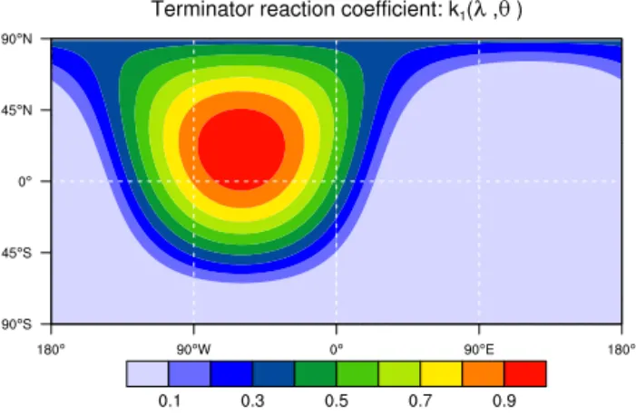
The reaction coefficient, k1, represents the photolytic breaking of molecule X2and can be represented as the co-sine of the solar zenith angle for when the sun’s zenith is at
Figure 1.Contour plot of the terminator-“like” reaction coefficient
k1(λ, θ )whereλandθare longitude and latitude, respectively.
k1(λ, θ )=max [0,sinθsinθc
+cosθcosθccos(λ−λc)], (9)
k2(λ, θ )=1, (10)
whereλandθ are longitude and latitude, respectively, and
(λc, θc)are chosen as (20◦N, 300◦E) to align with the flow field. The terminator is the continuous boundary between day and night regions. These reaction rates produce very steep gradients in the X species near the terminator. This setup is of direct application to the real atmosphere as the total chlo-rine in the stratosphere is conserved (except for molecular diffusion), while photolysis and chemical reactions partition the various components and lead to narrow gradients across the terminator.
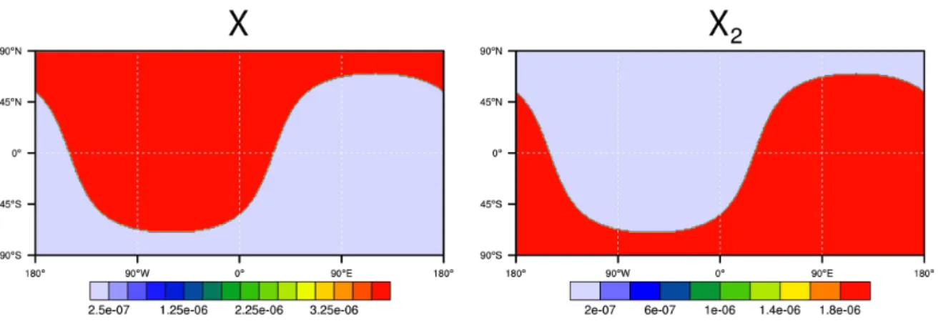
An analytic steady-state solution of the chemical concen-trations for the condition of no flow is derived in Appendix B. The initial condition is specified as being the steady-state so-lution under no flow (see Fig. 2). Reaction rates are quite rapid compared to the model time steps as shown in Ap-pendix C.
3 Transport operator and correlations
Let T be the discrete transport operator that advances, in time, the numerical solution to the passive and inert conti-nuity equation for species X and X2:
Dφ
Dt =0, φ=eX,eX2, (11)
at grid point or grid cell i(in this equation,eX refers to the volume mixing ratio of X (Andrews et al., 1987), which is related to the number density of X through scaling by the fixed ratio of the atomic weight of X to the molecular weight of dry air):
φin+1=φin+1ttracerT(φjn), j ∈H, φ=eX,eX2, (12) wherenis the time-level index,1ttracerthe time step for the transport operator, and His the set of indices defining the stencil required byT to updateφn
i. Note that the transport operator may not solve the prognostic equation forφin ad-vective form as used in Eqs. (4) and (5). For example, it is common practice for finite-volume schemes to base the dis-cretization on a flux-form formulation of the continuity equa-tion (here written without forcing terms):
∂(ρ φ)
∂t = −∇ ·(
vρ φ) , (13)
where ρ is air density. To deduce the mixing ratio from Eq. (13), one needs to solve the continuity equation for air. For a non-divergent wind field and an initial condition ofρ
that is constant, the exact solution forρ is that it remains constant in time and space. For the terminator test, in which we use a non-divergent flow field and constant initial con-dition forρ (if applicable), it has been found to be crucial to solve forρ rather than to prescribe the analytic solution forρ. Usually, a transport scheme using ρ φas a prognos-tic variable will not preserve aρ φ=constant initial condi-tion, whereas it will preserve a constant mixing ratio. So, if
ρ is analytically prescribed,φ will not be preserved in ar-eas where it would otherwise be constant. Such errors can be exacerbated by the terminator chemistry. For a fuller discus-sion of tracer–air coupling, see, e.g., Lauritzen et al. (2011) and Nair and Lauritzen (2010).
For the theoretical discussion, it is convenient to define the property “semi-linear”: a transport operatorT is semi-linear if it satisfies
T(aφi+b)=aT(φi)+bT(1)=aT(φi)+b, (14) for any constantsa andb (Lin and Rood, 1996; Thuburn and McIntyre, 1997). A semi-linear transport operator pre-serves linear correlation between two trace species. Note that the semi-linear property subsumes that the transport operator preserves a constant mixing ratio
T(b)=b. (15)
Since XTis simply the weighted sum of just two species, XT will be conserved in the numerical model ifT is semi-linear. The semi-linear property, however, does not imply that a weighted (linear) sum of more than two species is con-served (Lauritzen and Thuburn, 2012). The chemical reac-tions (Eqs. 1 and 2), even in discrete form, will preserve the sum of species. Consequently, a semi-linear transport opera-tor combined with the terminaopera-tor chemistry will produce no error in XT.
Figure 2.Contour plots of the steady-state solutions, assuming no flow, for X (left) and X2(right), respectively, computed from initial
conditions X=4.0×10−6and X2=0.
Lin and Rood (1996) show that their scheme, based on the widely used piecewise parabolic method (PPM; Colella and Woodward, 1984) for reconstructing sub-grid-scale tracer fields, preserves linear correlations. The CSLAM scheme (Lauritzen et al., 2010), also based on polynomials, preserves linear correlations (see the proof in Appendix A of Harris et al., 2010). An example of a scheme that is not semi-linear is the transport operator based on rational functions described in Xiao et al. (2002), due to the non-linearity of the recon-struction function.
Typically, transport operators are not applied in their unlimited versions in full models. Shape-preserving fil-ters are applied to ensure physically realizable solutions such as the prevention of negative mixing ratios or un-physical oscillations in the numerical solutions (e.g., Dur-ran, 2010). The filter method/algorithm depends on the advection scheme formulation and discretization. Finite-volume discretizations that are based on cell-average prog-nostic variables (ρφ) usually make use of either sub-grid-cell reconstruction function filters, e.g., van Leer type 1-D limiters (Lin et al., 1994), or flux-limiting methods such as flux-corrected transport (Zalesak, 1979). The reconstruc-tion filter can be applied for schemes that are based on La-grangian or Eulerian finite-volume discretizations, where the integration is based on swept areas (in either dimensionally split 1-D operators such as Lin and Rood, 1996, or fully 2-D) that span the domain without gaps or overlaps. Exam-ples of reconstruction function filters are Colella and Wood-ward (1984) and Lin and Rood (1996). Limiting through flux correction, where low-order shape-preserving fluxes are op-timally blended with higher-order fluxes, can only be ap-plied in flux-form schemes. For discretizations based on a non-conservative form (advective form), where the prognos-tic variables are mixing ratioφ rather thanρφ, tracer mass conservation is not inherent, and is usually restored a poste-riori with ad hoc methods (e.g., Priestley, 1993; Gravel and Staniforth, 1994). Since the mass-restoration algorithm may alterφ, the mass-fixer and shape-preservation algorithms are
intrinsically related. Usually, this problem is solved using optimization/variational methods (e.g., White and Dongarra, 2011). For methods where the prognostic variables are repre-sented by series expansions (e.g., Galerkin methods), shape preservation can also be enforced with optimization methods (e.g., Guba et al., 2014).
Shape-preserving filters may render an otherwise semi-linear transport operator non-semi-semi-linear. Some limiters, however, are semi-linear. For example, van Leer type 1-D limiters (Lin et al., 1994) preserve linear correlations (Lin and Rood, 1996). Flux-corrected transport limiters with and without selective limiting preserve linear correlations (Blossey and Durran, 2008; Harris et al., 2010). The lim-iter by Barth and Jespersen (1989) that scales the reconstruc-tion funcreconstruc-tions, so that it is within the range of the surround-ing cell average values, preserves linear correlations (Harris et al., 2010). Positive definite limiters that insure positivity-preservation and “clipping” algorithms that simply remove negative values (see, e.g., Skamarock and Weisman, 2009, for applications in a weather forecast model) are certain to violate linear correlations as the filter only affects the species that is about to become negative, and not the other species. Note that “clipping” may occur in the physical parameteri-zation package. A posteriori filters (e.g., optimiparameteri-zation-based shape-preserving filters) may or may not be semi-linear, and the details of the implementation can affect the semi-linearity (e.g., iteration thresholds, logic in the code).
We note that, instead of advecting each species separately by solving the advection equations in Eqs. (11) or (13) with
dis-tributions in the stratosphere. For idealized tests to evaluate how well families of species that add up to a constant are preserved, see, e.g., Lauritzen and Thuburn (2012).
4 Discrete terminator test
Coupling the chemistry parameterization with advection can be done in multiple ways. A common approach in weather/climate modeling is to update the species evolu-tion in time incrementally by first updating the mixing ra-tios with respect to sub-grid-scale forcings (chemistry) and then to apply the transport operator based on the chemistry-updated state (or in reverse order). Since the computation of the sub-grid-scale tendencies in full models is computa-tionally costly, the dynamical core (in this case, the transport scheme) is usually subcycled with respect to chemistry. For fast chemistry, this may be reversed.
A model will operate with a chemistry (physics) time step 1tchem, a tracer time step 1ttracer and a chemistry– transport (physics–dynamics) coupling time step 1tcpl. For example, in the default CAM-SE setup, 1ttracer=300 s,
1tchem=1800 s and1tcpl=600 s. Hence, the chemistry ten-dencies, FX andFX2, are computed every 30 min, and the species are updated every 600 s with the chemistry tenden-cies. A detailed description of the CAM-SE implementation of physics–dynamics coupling in terms of its namelist vari-ables is given in Appendix E.
It is, of course, up to the model developer to choose which coupling method and time step to use. To facilitate comparison, the model developer is encouraged to use the analytically computed forcing terms FX and FX2 given in Appendix F, and to use a chemistry (physics) time step of 1tchem=1800 s. The initial conditions are given by the steady-state asymptotic solutions Eqs. (B14) and (B15) with a mixing ratio of XT=4×10⁻⁶(Fortran code for the initial conditions is given in Appendix G and in the Supplement).
For simplicity, the velocity field for the transport opera-torT is prescribed. We use the deformational flow of Nair and Lauritzen (Case 2; 2010) that was also used in the stan-dard test case suite of Lauritzen et al. (2012, 2014). For completeness, the components of the non-divergent veloc-ity vector V(λ, θ, t ) and the stream function are repeated in Appendix A. The test is run for 12 days (or 5 non-dimensional time units) exactly as prescribed in Nair and Lauritzen (2010). Note that the test case methodology can be applied in any velocity field, including a full 3-D dynamical core.
5 Results
It is the purpose of this section to show exploratory termina-tor test results. An in-depth analysis of why the limiters do not preserve linear relations (and the derivation of possible remedies) is up to the scheme developers.
5.1 Model setup
Terminator test results are shown for two dynamical cores (transport schemes) available in the CAM: CAM-FV (Lin, 2004) and CAM-SE (Dennis et al., 2012), which are docu-mented within the framework of CAM in Neale et al. (2010). The transport scheme in CAM-FV is the widely used finite-volume scheme of Lin and Rood (1996). CAM-SE performs tracer transport using the spectral element method based on degree 3 polynomials. Further details on CAM-SE are given in Appendix H.
As discussed in detail in Nair and Lauritzen (2010) and briefly in Sect. 3, care must be taken in the handling of the tracer mixing ratio and tracer mass coupling for schemes that prognose tracer mass. In general, the transport scheme will not preserve a constant tracer density field (ρφ=constant), since the discrete divergence operator is non-zero despite the analytical wind field being non-divergent (zero divergence). However, the scheme will preserve a constant mixing ratio if
φis recovered fromρφby dividing the tracer density by the prognosed air densityρ. If one does not prognoseρand sim-ply specifies the analytic solution (ρ=constant), a constant mixing ratio will not be preserved.
For all simulations, the chemistry (physics) time step is
1tchem=1800 s. The horizontal resolution is approximately 1◦: for CAM-FV, that is the 0.9×1.25 configuration (192 latitudes and 288 longitudes) and, for CAM-SE, it is the NE30NP4 configuration in which there are 30×30 ele-ments on each cubed-sphere panel and 4×4 Gauss–Lobatto– Legendre (GLL) quadrature points in each element. The tracer time step1ttraceris 900 s for CAM-FV and 300 s for CAM-SE. During the tracer transport scheme time step, the analytic winds of Nair and Lauritzen (2010) are held constant following the CAM-Chem setup (Lamarque et al., 2012). Unless explicitly stated otherwise, the coupling time step for CAM-SE is1tcpl=600 and1tcpl=1800 for CAM-FV. For details on CAM chemistry–transport coupling, see Ap-pendix E.
The sample results shown next are divided into four sec-tions: first of all, baseline results for CAM-FV and CAM-SE using their default configurations. Next, results from experi-ments varying the limiter in CAM-SE are presented. Then, the consequences of using different chemistry–transport (physics–dynamics) coupling methods (in CAM-SE) are dis-cussed. Lastly, the results are quantified.
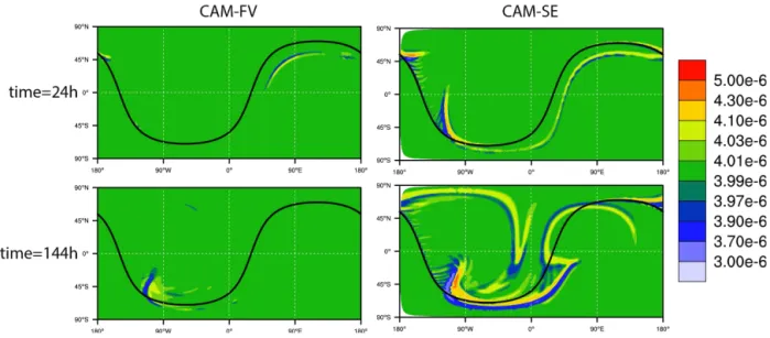
Figure 3.Contour plots of XTfor (left column) CAM-FV and for (right column) CAM-SE in ftype=0 configuration at day 1 (upper row)
and day 6 (lower row), respectively. Solid black line is the location of the terminator line. Note that the contour levels are not linear.
Lagrangian trajectories of the prescribed flow. This is most visible for CAM-SE at day 6 (see Fig. 3 and/or the anima-tions in the Supplement).
CAM-FV transport is based on the dimensionally split Lin and Rood (1996) scheme. The scheme produces errors in XTsince the limiter used in CAM-FV (described in Ap-pendix B of Lin, 2004) does not strictly conserve linear rela-tions. The errors appear to be largest when the flow is aligned with the terminator at a 45◦angle (see the animation in the Supplement). In that situation, the dimensionally split ap-proach is most challenged; the shape-preserving limiter is not strictly shape-preserving in the cross direction since the one-dimensional limiters are only applied in the coordinate directions (Lauritzen, 2007).
CAM-SE does not preserve linear relations either and the errors in XT are about an order of magnitude larger than CAM-FV. The CAM-SE limiter is optimization based (us-ing least squares) and guarantees no under- or over-shoots at the element level while maintaining mass conservation at the element level (Guba et al., 2014). While the optimization-based limiter preserves linear relations with exact arithmetic, its present implementation in CAM-SE does not lead to such preservation (most likely due to iteration thresholds, if-statements, etc., that can be non-linear).
To further understand this behavior, we have performed some tests (not shown) turning the chemistry off and ad-vecting linearly correlated cosine hills and linearly correlated step functions. The cosine hills areC0continuous (the func-tion is continuous but its derivatives are not) and the limiter exactly preserves the linear relationship. For the step func-tions, which are discontinuous distribufunc-tions, the correlation preservation is only maintained up to O(10−8) due to an
O(10−8)overshoot in one of the tracers. So, the advection operator introduces anO(10−8)error. The terminator
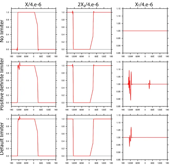
chem-Figure 4.Contour plot of XTat day 1 using CAM-SE in ftype=1
configuration where (upper) no limiter, (middle) a positive definite limiter, and the default CAM-SE limiter are applied, respectively. The solid black line depicts the location of the terminator line. Note that the contour levels are not linear.
Figure 5.Cross sections of day 1 (left column) X, (middle column) 2×X2, and (right column) XTat 45◦S based on CAM-SE with (top row)
no limiter, (middle row) positive definite limiter, (lower row) and default limiter, respectively. Results are normalized by 4×10⁻⁶(the initial value of XT).
trace down exactly where in the implementation this error is introduced and to find a remedy. The terminator test is de-signed to enable scheme developers to test their scheme in setups that are directly relevant to some of the issues seen in chemistry application. In this particular case, the terminator test clearly exacerbates small errors in correlation preserva-tion that may be easily overlooked in inert transport testing (such as the tests in Lauritzen et al., 2012).
5.3 CAM-SE: limiter experiments
In addition to the quasi-monotone mass-conservative limiter used by default in CAM-SE, the model has options for per-forming tracer advection without any limiter and with a pos-itive definite limiter. Results for terminator test runs using
When using a positive definite limiter, Gibbs phenomena are eliminated near the base of the terminator, but not near the maximum. This obviously violates linear relations and pro-duces large errors in XT. Similar results are expected from mass-filling algorithms in which negative values are simply set to 0. This emphasizes the importance of using carefully designed limiters in transport schemes for applications in which preservation of linear pre-existing relations is impor-tant, e.g., chemistry applications (for a fuller discussion, see, e.g., Lauritzen and Thuburn, 2012).
5.4 CAM-SE: chemistry–tracer (physics–dynamics) coupling experiments
As explained in Sect. 4, the tracer transport (dynamics) and chemistry (physics) can be coupled in various ways. Here, we discuss results based on different coupling time steps,1tcpl, in CAM-SE.
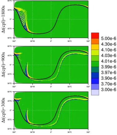
In Fig. 6, XT is shown using 1tcpl=1800 s, 1tcpl= 600 s, and 1tcpl=300 s, respectively1. In all experiments, the tracer time step nd chemistry time step are held fixed:
1ttracer=300 s and 1tchem=1800 s, respectively. The ex-periments evaluate the sensitivity to coupling time-step size, in other words, how often the species are adjusted with chem-istry tendencies.
Near the western edge of the terminator (located at approx-imately 130◦W in Fig. 5) where the gradients are steepest, the errors in XTare largest for1tcpl=1800 s. The chemistry adjustments that steepen the gradients are largest at the west-ern edge and consequently produce states that challenge the limiters more. When the chemistry tendency is added gradu-ally throughout the tracer transport, the errors are reduced as
1tcplis decreased.
At the eastern edge of the terminator (located at approxi-mately 30◦E in Fig. 5), the gradients are less steep compared to the western edge. In fact, the location of the gradient near the eastern edge propagates (see animation in Supplement), whereas the gradients at the western edge of the terminator are static in space. The chemistry tendencies in this area are not stationary in space and are weaker, so the transport signal is larger. This means that, for any given point in the eastern area, the state used for computing the chemistry tendencies changes during the tracer subcycling. As a result, the gradi-ents will have propagated during the transport step, but the chemistry tendencies will steepen gradients in the “old” lo-cation. This “inconsistency” is present with1tcpl6=1tchem. For1tcpl=1800 s, the chemistry update is based on the “cor-rect” in time state. The temporal inconsistency in the state used for computing chemistry tendencies for 1tcpl=600 s and 1tcpl=300 s produces an increase in errors near the eastern edge of the terminator compared to1tcpl=1800 s.
1In terms of the CAM-SE namelist, these configurations
cor-respond to (a) ftype=1, nsplit=1, rsplit=6, (b) ftype=0, nsplit=2, rsplit=3, and (c) ftype=0, nsplit=6, rsplit=1.
Figure 6. Contour plots of XT at day 1 using CAM-SE based
on (upper) 1tcpl=1800 s, (middle) 1tcpl=900 s, and (lower)
1tcpl=300 s, respectively. In all simulations, the tracer and
chem-istry time step is constant:1ttracer=300 s and1tchem=1800 s,
respectively.
Physical parameterization packages may contain code that sets negative mixing ratios to 0. Or, similarly, there may be code that prevents tendencies from being added to the state if it is 0 or negative. The terminator test may be a useful tool to diagnose such alternations in large complicated codes. 5.5 Quantification of XTerrors
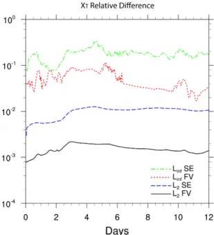
To quantify the errors introduced in the terminator test, we suggest computing standard error norms for XT. The global normalized error norms used areℓ2(t )andℓ∞(t )(e.g., Williamson et al., 1992):
ℓ2(t )= s
I[(XT(t )−XT(0))2]
I[(XT(0))2] , (16)
ℓ∞=
max∀λ,θ|XT(t )−XT(0)| max∀λ,θ|XT(0)|
, (17)
I (φ)= 1
4π
2π Z
0 π/2 Z
−π/2
φ (λ, θ, t )cosθdλdθ. (18)
As a reference, we show the time evolution ofℓ2(t )and
ℓ∞(t )for CAM-FV and CAM-SE in Fig. 7.
6 Conclusions
A simple idealized toy chemistry test case is defined. It con-sists of advecting two reactive species (X and X2) in the Nair and Lauritzen (2010) flow field. The simplified non-linear chemistry creates strong gradients in the species similar to what is observed for photolysis-driven species in the strato-sphere. The forcing terms for the continuity equations for X and X2are computed analytically over one time step (assum-ing no advection) and Fortran codes for comput(assum-ing the forc-ing terms are provided in the Supplement. Hence, model de-velopers who have already set up the standard test case suite of Lauritzen et al. (2012) can, with modest effort, set up the terminator test by adding the forcing terms to their codes. As in the test case of Nair and Lauritzen (2010), this forced advection problem has an analytic solution.
The toy chemistry, by design, does not disrupt pre-existing linear relations between the species. So, the only source of error is from the transport scheme and/or the chemistry– transport (physics–dynamics) coupling. The terminator test is set up so that XT is a constant, so any deviation from constancy is an error in the preservation of linear correla-tions. Many transport schemes preserve linear relations when no shape-preserving limiter/filter is applied and are there-fore not challenged with respect to conserving XT. However, many shape-preserving limiters/filters render the transport scheme non-conserving with respect to XT. While preser-vation of linear correlations can indeed be verified in inert advection setups, the terminator chemistry exacerbates the non-conservation problem through the constant forcing that creates very steep gradients. It is demonstrated in this paper that the terminator test is useful for challenging the limiters with strong grid-scale forcing. In particular, it is shown that positive definite limiters severely disrupt linear correlations near the terminator.
In addition, the terminator test assesses the accuracy of chemistry–tracer (physics–dynamics) coupling methods in an idealized setup. Different coupling methods (such as those available in CAM-SE) lead to different distributions of XT. Also, a chemistry–transport (physics–dynamics) coupling layer or the physical parameterization package may contain code that sets negative mixing ratios to 0 and/or contain if-statements that prevent tendencies being added to the state if it is 0 or negative. The terminator test may be a useful tool to diagnose such alternations in large complicated codes.
Figure 7.Time evolution of standard error normsℓ2andℓ∞for XT using the CAM-FV and CAM-SE dynamical cores. Note that
theyaxis is logarithmic.
The terminator test is easily accessible to advection scheme developers from an implementation perspective since the software engineering associated with extensive parame-terization packages is avoided. The test forces the model de-veloper to consider how their scheme is coupled to sub-grid-scale parameterizations and, if solving the continuity equa-tion in flux form, forces the developer to consider tracer– air mass coupling. Also, the idealized forcing proposed here has an analytic formulation, and the continuous set of forced transport equations has, contrary to the Brusselator forcing, an analytic solution for the weighted sum of the correlated species, irrespective of the flow field.
Appendix A: Idealized flow field
In the terminator test, we use the deformational flow of Nair and Lauritzen (Case 2; 2010). The components of the non-divergent velocity vectorV(λ, θ, t )and the stream function
u= −∂ψ
∂θ, (A1)
v= 1
cosθ ∂ψ
∂λ, (A2)
are given by
u(λ, θ, t )=10R
T sin
2(λ′)sin(2θ )cos π t
T
+2π R
T cos(θ ) (A3)
v(λ, θ, t )=10R T sin(2λ
′)cos(θ )cos π t
T
, (A4)
ψ (λ, θ, t )=10R
T sin
2(λ′)cos2(θ )cos π t
T
−2π R
T sin(θ ), (A5)
respectively, whereλis longitude,θis latitude,tis time and the underlying solid-body rotation is added through the trans-lationλ′=λ−2π t /T. The period of the flow isT =12 days andR=6.3172×10⁶m (in non-dimensional unitsT =5 and
R=1). Schemes based on characteristics, e.g., Lagrangian and semi-Lagrangian schemes, may use the semi-analytic trajectory formulas given in (Nair and Lauritzen, 2010). Note that it is not necessary to use an analytic flow field for this test case setup. In fact, one may use winds from a weather or climate model simulation.
Appendix B: Analytic solution for no flow
To gain more insight into the toy chemistry (and to formulate “spun-up” initial conditions), it is useful to consider the spe-cial case of no flow. Forv=0, the prognostic equations for X and X2(Eqs. 4 and 5, respectively) can be solved analyt-ically. Assume the reaction rates are positive (and non-zero fork2),
k1≥0, (B1)
k2>0 (B2)
and the mixing ratios are non-negative,
X(0)≥0, (B3)
X2(0)≥0. (B4)
From the kinetic Eqs. (4) and (5) above, as well as the conservation Eq. (3), we can write
dX
dt =k1(XT−X)−2k2XX. (B5)
For (algebraic) convenience, define the quantities
r= k1
4k2
, (B6)
D=pr2+2rXT, (B7)
E(t )=e−4k2Dt. (B8)
Completing the square on the right-hand side leads to the expression
dX
dt = −2k2[(X+r)
2−D2]. (B9)
The right-hand side can be factored, and the following par-tial fraction expansion can be constructed:
dX
(X+r)−D−
dX
(X+r)+D= −4Dk2dt. (B10)
Integration of each of these terms from time t=0 to t
yields the expression ln
(X(t )+r−D)(X(0)+r+D) (X(t )+r+D)(X(0)+r−D)
= −4Dk2t, (B11) leading to the solutions Eq. (B12). The analytic solution for X(t )is
X(t )= (
D(X(0)(X(0)++r)(1r)(1+−E(t ))E(t ))++D(1D(1−+E(t ))E(t ))−r ifr >0,
X(0)
1+2k2tX(0) ifr=0. (B12) X2(t )=1
2(XT−X(t )) . (B13)
For long times, X(t )and X2(t )converge to the steady-state solutions
limt→∞X(t )=D−r, (B14)
limt→∞X2(t )= 1
2(XT−D+r) , (B15)
Appendix C: Local linear convergence
If the flow is slow compared to the rate at which the chem-istry returns to equilibrium, then the concentrations will stay near the steady-state solution derived in Appendix B. Under these conditions, the rate of convergence to the steady-state solution can be computed. For convenience, define Xsas the right-hand side of Eq. (B14). From Eq. (B5), a perturbation from steady state,ǫ(t )=X(t )−Xs, can be seen to solve the equation
dǫ(t )
dt = −k1ǫ(t )−4k2Xsǫ(t )−2k2ǫ
2(t ), (C1)
which implies a locally linearized convergence rate forǫ(t )
of
−k1−4k2Xs. (C2)
Since the maximum of X is 4×10⁻⁶andk2=1, this con-vergence rate is dominated byk1∈ [0,1]. It is clear that the reaction convergence is very rapid in regions of sunlight and much slower in dark regions. Peak rates in this computation are 1 s−1.
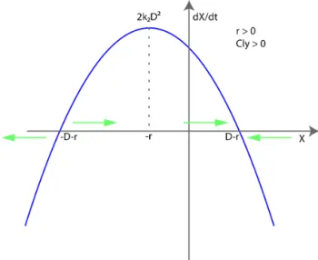
Appendix D: Stability of chemical kinetics
Relation Eq. (B9) is plotted in Figs. D1 and D2. As can be seen in Fig. D1, fork1>0, X converges toD−r. Fork1=0, Fig. D2 shows that X converges to 0 for values greater than 0, but diverges for X<0. While X should never be negative, numerical errors can lead to negative values. This divergence is slow, in the sense that the divergence is algebraic, as can be seen in Eq. (B12). The divergence is also slow in the sense that the time required to double a negative X concentration is
t2= − 1
4k2X. (D1)
Thus, for very small (negative) X, the time will have to be particularly large. However, for time of 2·t2, the solution is singular, reaching a value of−∞.
Appendix E: CAM-SE chemistry–tracer (physics–dynamics) coupling
The different levels of subcycling used in CAM-SE are explained via pseudo-code in Algorithm 1 using CAM-SE namelist conventions: nsplit and rsplit. The outer time-stepping loop starts with a call to chemistry that computes the chemistry tendencies over the entire chemistry time step
1tchem. The full chemistry tendencies are divided into nsplit adjustments of equal size and, in each iteration of the nsplit loop, the adjustments are added to the state. The tracer transport scheme may not be stable on the chemistry time
Figure D1.Whenk1>0, or equivalentlyr >0, there is a single
stable limit point. X will converge toD−ras long as X>−D−r.
Figure D2.Whenk1=0, or equivalentlyr=0, X converges to 0, but if, for some numerical reason, X is made negative, the kinetic equations will make the concentrations even more negative.
Algorithm 1 Pseudo-code explaining the different levels of subcycling and chemistry–transport (physics–dynamics) coupling used in CAM-SE.
Outer loop advances solution1tchemin time:
fort=1,2, . . .do
Compute chemistry tendenciesFi,i=X,X2
forns=1,2, . . .,nsplitdo
Update state with chemistry/physics tendencies:
Ci=Ci+1tnsplitchemFi,i=X,X2
forrs=1,2, . . .,rsplitdo
subcycling of tracer advection:
Ci=Ci+nsplit1tchem×rsplitT(Ci),i=X,X2
step (1tchem) or the coupling/adjustment time step (1tcpl=
1tchem/nsplit), so it must be subcycled with respect to the chemistry adjustments. The number of iterations of the tracer transport subcycling loop is rsplit. Note that, since the nsplit and rsplit loops are nested, the tracer time step is1ttracer=
1tchem (nsplit×rsplit).
We distinguish between the nsplit=1 and nsplit>1 con-figurations and refer to them as ftype=1 and ftype=0, re-spectively, based on CAM-SE namelist terminology (ftype refers to forcing type)2. In the CAM code, if ftype=1, the state is updated with chemistry (physics) tendencies in the physics code, whereas for ftype=0, the adjustments take place in the dynamical core. CAM-FV uses an ftype=1 con-figuration (with the caveat that the chemistry tendencies are added after the transport is complete) and CAM-SE supports both ftype=0 and ftype=1. The current default CAM-SE uses ftype=0, where the tendencies are split into nsplit equal-sized adjustments.
In full model runs, if the physics time step is large, the ftype=1 coupling method may produce large physics ten-dencies that drive the state much out of balance. When the dynamical core is given the physics updated state that is strongly (and locally) out of balance, the dynamical core may produce excessive gravity waves. To alleviate this, one may choose to update the state with respect to physics tendencies throughout the tracer subcycling. This approach of adding the physics tendencies as several equal-sized adjustments is the ftype=0 configuration that was explained above.
For the 1◦ setup (NE30NP4), we use the stan-dard/recommended configuration with rsplit=3 and nsplit=2 (see the pseudo-code in Algorithm 1), so that for every third tracer time step, half of the chemistry tenden-cies are added to the state. In terms of tracer, chemistry and coupling time steps, this configuration corresponds to 1ttracer=300 s, 1tchem=1800 s and 1tcpl=600 s. CAM-FV uses ftype=1 configuration where the chemistry tendencies are added once3. For CAM-FV, 1ttracer=900 s,
1tchem=1800 s and1tcpl=1800 s.
2When running the 3-D CAM-SE dynamical core, nsplit defines
the vertical remapping time step; if ftype=0, then nsplit also de-fines the adjustment time step, whereas if ftype=1, then nsplit only defines the remapping time step, as the full adjustments are added at the beginning of dynamics only.
3Note however that, in CAM-FV, the tendencies are added after
tracer transport and not before.
Appendix F: Analytic chemical forcing term
The analytic solution of the equations leads to an explicit solution for the change in concentrations during a time step with no flow.
FXn= −L1tchem
× (X
n−D+r)(Xn+D+r) 1+E(1tchem)+1tchemL1tchem(Xn+r)
, (F1)
where Xn is the value of X at the beginning of thenth time step,
L1tchem =
1−e−4k2D1tchem
D1tchem ifD >0
4k2 ifD=0,
(F2)
and, by conservation,
FXn 2 = −
1 2F
n
X. (F3)
In implementation,L1tchem needs some care. As 4k2D1t approaches machine precision, it is useful to simply use the formula forD=0 rather than the expression forD >0.
Appendix G: Fortran code
In terms of Fortran code, the analytical forcing is given by ! dt is size of chemistry/physics ! time step
XT = X + 2.0*X2
r = k1/(4.0*k2)
d = sqrt(r*r + 2.0*r*XT) e = exp(-4.0*k2*d*dt)
if(abs(d*k2*dt).gt. 1e-16) el = (1.0-e)/(d*dt) else
el = 4.0*k2 endif
f_X = -el * (X-d+r) * (X+d+r)/ (1.0 + e + dt*el*(X+r))
f_X2 = -f_X/2.0
The reaction rates are defined by
! k1 and k2 are reaction rates k1_lat_center = 20.0 ! degrees k1_lon_center = 300.0 ! degrees k1 = max(0.d0,
sin(lat)*sin(k1_lat_center) + cos(lat)*cos(k1_lat_center)
The initial condition is defined by XT = 4.0e-6
r = k1/(4.0*k2)
d = sqrt(r*r + 2.0*XT*r)
X = d-r
X2 = XT/2.0 - (d-r)/2.0
These specifications are implemented in Fortran code in the Supplement.
Appendix H: CAM-SE time-stepping
The Supplement related to this article is available online at doi:10.5194/gmd-8-1299-2015-supplement.
Acknowledgements. NCAR is sponsored by the National Science Foundation (NSF). Jean-François Lamarque, Andrew Conley and Francis Vitt were partially funded by the Department of Energy (DOE) Office of Biological & Environmental Research under grant number SC0006747. Mark Taylor was supported by the Depart-ment of Energy Office of Biological and EnvironDepart-mental Research, work package 12-015335, “Applying Computationally Efficient Schemes for BioGeochemical Cycles”. Thanks to Oksana Guba for discussions on the CAM-SE limiter. The authors are grateful to Michael Prather for the many discussions on simplified chemistry. We thank the reviewers for their constructive comments that greatly improved the manuscript.
Edited by: F. O’Connor
References
Anderson, J., Toohey, D., and Brune, W.: Free radicals within the Antarctic vortex: the role of CFCs in Antarctic ozone loss, Sci-ence, 251, 39–46, doi:10.1126/science.251.4989.39, 1991. Andrews, D. G., Holton, J. R., and Leovy, C. B.: Middle
atmo-sphere dynamics, Academic Press, San Diego, 1987.
Barth, T. and Jespersen, D.: The design and application of upwind schemes on unstructured meshes, in: Proc. AIAA 27th Aerospace Sciences Meeting, Reno, 1989.
Blossey, P. N. and Durran, D. R.: Selective monotonicity preser-vation in scalar advection, J. Comput. Phys., 227, 5160–5183, 2008.
Brasseur, G. and Solomon, S.: Aeronomy of the Middle Atmo-sphere, Springer, 3rd Edn., 2005.
Colella, P. and Woodward, P. R.: The Piecewise Parabolic Method (PPM) for gas-dynamical simulations, J. Comput. Phys., 54, 174–201, 1984.
Dennis, J. M., Edwards, J., Evans, K. J., Guba, O., Lauritzen, P. H., Mirin, A. A., St-Cyr, A., Taylor, M. A., and Worley, P. H.: CAM-SE: A scalable spectral element dynamical core for the Com-munity Atmosphere Model, Int. J. High Perform. C., 26, 74–89, doi:10.1177/1094342011428142, 2012.
Douglass, A. R., Stolarski, R. S., Strahan, S. E., and Connell, P. S.: Radicals and reservoirs in the GMI chemistry and transport model: Comparison to measurements, J. Geophys. Res., 109, D16302, doi:10.1029/2004JD004632, 2004.
Durran, D.: Numerical Methods for Fluid Dynamics: With Appli-cations to Geophysics, vol. 32 of Texts in Applied Mathematics, Springer, 2nd Edn., 516 pp., 2010.
Edouard, S., Legras, B., and Zeitlin, V.: The effect of dynamical mixing in a simple model of the ozone hole, J. Geophys. Res., 101, 2156–2202, doi:10.1029/96JD00856, 1996.
Gravel, S. and Staniforth, A.: A mass-conserving semi-Lagrangian scheme for the shallow-water equations, Mon. Wea. Rev., 122, 243–248, 1994.
Guba, O., Taylor, M., and St-Cyr, A.: Optimization-based limiters for the spectral element method, J. Comput. Phys., 267, 176–195, doi:10.1016/j.jcp.2014.02.029, 2014.
Harris, L. M., Lauritzen, P. H., and Mittal, R.: A flux-form ver-sion of the Conservative Semi-Lagrangian Multi-tracer transport scheme (CSLAM) on the cubed sphere grid, J. Comput. Phys., 230, 1215–1237, doi:10.1016/j.jcp.2010.11.001, 2010.
Kinnmark, I. P. and Gray, W. G.: One step integration methods with maximum stability regions, Math. Comput. Simulat., 26, 87–92, doi:10.1016/0378-4754(84)90039-9, 1984a.
Kinnmark, I. P. and Gray, W. G.: One step integration methods of third-fourth order accuracy with large hyperbolic stability lim-its, Math. Comput. Simulat., 26, 181–188, doi:10.1016/0378-4754(84)90056-9, 1984b.
Kristensen, L., Lenschow, D. H., Gurarie, D., and Jensen, N. O.: A simple model for the vertical transport of reactive species in the convective atmospheric boundary layer, Bound.-Lay. Meteorol., 134, 195–221, doi:10.1007/s10546-009-9443-x, 2010.
Lamarque, J.-F., Emmons, L. K., Hess, P. G., Kinnison, D. E., Tilmes, S., Vitt, F., Heald, C. L., Holland, E. A., Lauritzen, P. H., Neu, J., Orlando, J. J., Rasch, P. J., and Tyndall, G. K.: CAM-chem: description and evaluation of interactive at-mospheric chemistry in the Community Earth System Model, Geosci. Model Dev., 5, 369–411, doi:10.5194/gmd-5-369-2012, 2012.
Lander, J. and Hoskins, B. J.: Believable scales and parameterizations in a spectral transform model, Mon. Wea. Rev., 125, 292–303, doi:10.1175/1520-0493(1997)125<0292:BSAPIA>2.0.CO;2, 1997.
Lauritzen, P. H.: A stability analysis of finite-volume advection schemes permitting long time steps, Mon. Weather Rev., 135, 2658–2673, 2007.
Lauritzen, P. and Thuburn, J.: Evaluating advection/transport schemes using interrelated tracers, scatter plots and numeri-cal mixing diagnostics, Q. J. Roy. Meteor. Soc., 138, 906–918, doi:10.1002/qj.986, 2012.
Lauritzen, P. H., Nair, R. D., and Ullrich, P. A.: A conserva-tive semi-Lagrangian multi-tracer transport scheme (CSLAM) on the cubed-sphere grid, J. Comput. Phys., 229, 1401–1424, doi:10.1016/j.jcp.2009.10.036, 2010.
Lauritzen, P. H., Ullrich, P. A., and Nair, R. D.: Atmospheric trans-port schemes: desirable properties and a semi-Lagrangian view on finite-volume discretizations, in: Numerical Techniques for Global Atmospheric Models, Lecture Notes in Computational Science and Engineering, edited by: Lauritzen, P. H., Nair, R. D., Jablonowski, C., and Taylor, M., Springer, 80 pp., 2011. Lauritzen, P. H., Skamarock, W. C., Prather, M. J., and
Tay-lor, M. A.: A standard test case suite for two-dimensional lin-ear transport on the sphere, Geosci. Model Dev., 5, 887–901, doi:10.5194/gmd-5-887-2012, 2012.
Lin, S.-J.: A “vertically Lagrangian” finite-volume dynamical core for global models, Mon. Weather Rev., 132, 2293–2307, 2004. Lin, S.-J. and Rood, R. B.: Multidimensional flux-form
semi-Lagrangian transport schemes, Mon. Weather Rev., 124, 2046– 2070, 1996.
Lin, S.-J., Chao, W. C., Sud, Y. C., and Walker, G. K.: A class of the van Leer-type transport schemes and its application to the moisture transport in a general circulation model, Mon. Weather Rev., 122, 1575–1593, 1994.
Nair, R. D. and Jablonowski, C.: Moving vortices on the sphere: a test case for horizontal advection problems, Mon. Weather Rev., 136, 699–711, 2008.
Nair, R. D. and Lauritzen, P. H.: A class of deformational flow test cases for linear transport problems on the sphere, J. Comput. Phys., 229, 8868–8887, doi:10.1016/j.jcp.2010.08.014, 2010. Nair, R. D. and Machenhauer, B.: The mass-conservative
cell-integrated semi-Lagrangian advection scheme on the sphere, Mon. Weather Rev., 130, 649–667, 2002.
Neale, R. B., Chen, C.-C., Gettelman, A., Lauritzen, P. H., Park, S., Williamson, D. L., Conley, A. J., Garcia, R., Kinnison, D., Lamarque, J.-F., Marsh, D., Mills, M., Smith, A. K., Tilmes, S., Vitt, F., Cameron-Smith, P., Collins, W. D., Iacono, M. J., Easter, R. C., Ghan, S. J., Liu, X., Rasch, P. J., and Taylor, M. A.: Description of the NCAR Community Atmosphere Model (CAM 5.0), NCAR Technical Note, National Center of Atmospheric Re-search, 2010.
Prather, M. and Jaffe, A. H.: Global impact of the Antarctic ozone hole: Chemical propagation, J. Geophys. Res., 95, 3473, doi:10.1029/JD095iD04p03473, 1990.
Priestley, A.: A quasi-conservative version of the semi-Lagrangian advection scheme, Mon. Wea. Rev., 121, 621–632, doi:10.1175/1520-0493(1993)121<0621:AQCVOT>2.0.CO;2, 1993.
Prigogine, I.: From Being to Becoming: Time and Complexity in the Physical Sciences, W. H. Freeman & Co, San Francisco, 1981. Prigogine, I. and Lefever, R.: Symmetry-breaking
instabili-ties in dissipative systems, J. Chem. Phys., 48, 1695–1700, doi:10.1063/1.1668896, 1968.
Pudykiewicz, J. A.: Numerical solution of the reaction-advection-diffusion equation on the sphere, J. Comput. Phys., 213, 358– 390, doi:10.1016/j.jcp.2005.08.021, 2006.
Pudykiewicz, J. A.: On numerical solution of the shal-low water equations with chemical reactions on icosahe-dral geodesic grid, J. Comput. Phys., 230, 1956–1991, doi:10.1016/j.jcp.2010.11.045, 2011.
Salawitch, R. J., Canty, T., Müller, R., Santee, M. L., Schofield, R., Stimpfle, R. M., Stroh, F., Toohey, D. W., and Urban, J.: Sect. 3. Workshop Report: The Role of Halogen Chemistry in Polar Stratospheric Ozone Depletion, in: Workshop for an Initiative under the Stratospheric Processes and Their Role in climate (SPARC) Project of the World climate Research Programme, June 2008, Cambridge, UK, 2009.
Skamarock, W. C. and Weisman, M. L.: The impact of positive-definite moisture transport on NWP precipitation forecasts, Mon. Weather Rev., 137, 488–494, doi:10.1175/2008MWR2583.1, 2009.
Spiteri, R. and Ruuth, S.: A new class of optimal high-order strong-stability-preserving time discretization methods, SIAM J. Numer. Anal., 40, 469–491, doi:10.1137/S0036142901389025, 2002.
Strahan, S. E., Douglass, A. R., Stolarski, R. S., Akiyoshi, H., Bekki, S., Braesicke, P., Butchart, N., Chipperfield, M. P., Cugnet, D., Dhomse, S., Frith, S. M., Gettelman, A., Hardiman, S. C., Kinnison, D. E., Lamarque, J.-F., Mancini, E., Marchand, M., Michou, M., Morgenstern, O., Nakamura, T., Olivi , D., Paw-son, S., Pitari, G., Plummer, D. A., Pyle, J. A., Scinocca, J. F., Shepherd, T. G., Shibata, K., Smale, D., Teyssèdre, H., Tian, W., and Yamashita, Y.: Using transport diagnostics to understand chemistry climate model ozone simulations, J. Geophys. Res., 116, 2156–2202, doi:10.1029/2010JD015360, 2011.
Thuburn, J. and McIntyre, M.: Numerical advection schemes, cross-isentropic random walks, and correlations between chemical species, J. Geophys. Res., 102, 6775–6797, 1997.
Turing, A.: The chemical basis of morphogenesis, Philos. T. R. Soc. Lon. B, 37–72, 1952.
White, J. B. and Dongarra, J. J.: Performance High-Resolution Semi-Lagrangian Tracer Transport on a Sphere, J. Comput. Phys. 230, 6778–6799, 2011.
Williamson, D. L., Drake, J. B., Hack, J. J., Jakob, R., and Swarz-trauber, P. N.: A standard test set for numerical approximations to the shallow water equations in spherical geometry, J. Comput. Phys., 102, 211–224, 1992.
Xiao, F., Yabe, T., Peng, X., and Kobayashi, H.: Conser-vative and oscillation-less atmospheric transport schemes based on rational functions, J. Geophys. Res., 107, 4609, doi:10.1029/2001JD001532, 2002.