THE SIGNIFICANCE OF
TRAVELLER’S
ROUTE
KNOWLEDGE FOR CHOICE OF COMMUTING
MODE OF TRANSPORT
Lukasz Kruk
ii The Significance of Traveller’s Route Knowledge for Choice of Commuting Mode of
Transport
Dissertation supervised by:
Lledó Museros Cabedo
Werner Kuhn
Marco Painho
iii ACKNOWLEDGEMENTS
This thesis deals as much with geographic information as with psychological and
cognitive approaches to such information. This is inspired by some of the classes
about the nature of geographic information I have attended during the course of
the MSc in Geospatial Technologies programme as well as my Mother’s, Prof.
iv ABSTRACT
Travelling in a city is an essential part of everyone’s life, whether it is the routine daily commute or navigating to a previously unknown place, and can be
accomplished with a variety of means of transport. This thesis explores how
personal, first-hand route knowledge influences choice of mode of transport. This is
motivated by the premise that human-oriented approach for computer systems
design can be of significant benefit to the user. Public (bus, train, tram, metro) and
private (bicycle, car, on foot) means of transport are considered and compared.
Collected survey data analysed with a logistic regression method does not show any
relationship between route knowledge and choice of mode of transport.
KEYWORDS
Route knowledge
Wayfinding
Transport mode choice
Mental map
v INDEX
Acknowledgements ... iii
Abstract ... iv
Keywords... iv
Index of figures ... vi
1. Introduction ... 1
1.1. Overview and motivation ... 1
1.2. Aim and approach ... 2
2. Background and literature review ... 4
2.1. Cognitive science ... 4
2.2. Representations ... 6
2.3. Scale ... 7
2.4. Environment ... 9
2.5. Cognitive spaces ... 10
2.6. Mental map ... 16
2.7. Related work ... 20
3. Methodology: data collection and analysis ... 23
3.1. Questionnaire ... 24
3.2. Data pre-processing ... 27
3.3. Exploratory analysis ... 28
3.4. Statistical analysis ... 35
3.5. Particular examples and geographic visualisation ... 37
3.6. Partial conclusions ... 40
4. Formalisation ... 42
4.1. Ontology extension ... 43
4.2. Future work – simulation extension ... 44
5. Conclusions ... 45
6. Appendix 1 – questionnaire ... 46
6.1. English ... 46
6.2. Polish ... 46
6.3. Spanish ... 47
7. Appendix 2 – questionnaire results ... 48
vi INDEX OF FIGURES
Figure 1 Cognitive spaces (adapted from: Montello 1993) ... 15
Figure 2 Travel distance histogram. ... 30
Figure 3 Distance against route familiarity box plot ... 31
Figure 4 Transport mode dependence on distance box plot. ... 33
Figure 5 Breakdown of transport modes according to distance ... 34
Figure 6 Route knowledge plotted against the route length. ... 34
Figure 7 Unknown (left) and known (right) routes broken down into various modes of transport. Vertical axis normalised for comparison. ... 35
Figure 8 Trips in the Tricity, Poland area. ... 38
Figure 9 Trips in the Münster, Germany area... 38
Figure 10 Münster walking and cycling trips. X axis represents distance, Y axis represents route familiarity. ... 39
1 1. INTRODUCTION
Travelling in our own city is an everyday activity each of us undertakes. A number of
decisions are made and a lot of considerations have to be taken into account for
every commute. Questions such as: where is the start and the end of the trip? what
is the trip length and what means of transport are available between them? what
would be the preferred mean of transport? what is the route itself like? are only
some of those considerations and they describe the focus of this thesis. The
interplay between these factors is the specific topic for data collection and analysis.
Some of the fundamental concepts employed in this paper are directly related to
National Center for Geographic Information and Analysis’ Research Initiative 21:
Formal Models of the Common Sense Geographic Worlds (Mark, Egenhofer, &
Hornsby, 1997) and the “Naive Geography” paper (Egenhofer & Mark, 1995). The
latter is also an inspiration for the interest in the topic.
1.1. OVERVIEW AND MOTIVATION
Geographic Information Systems (GIS) are relatively new tools that are used to deal
with spatial information. Their origins are dated back to 1960’s, but the bodies of
knowledge on which they build, such as geography and cartography, stem from
ancient times. Some of psychological concepts are just as relevant today as when
they were first published centuries ago. And yet, even now – or perhaps especially
now – we still struggle with the very nature of the data and information we are
dealing with. The human cognitive and spatial reasoning mechanisms are very
sophisticated and have been a subject of extensive research throughout decades
(Tolman, 1948)(Piaget, 1964)(Montello, 1993). GISs however lack similar
capabilities. What geographers used to take for granted and what people
effortlessly deal with on a daily basis using common sense – requires explicit
2 One of spatial tasks that come naturally and often unconsciously to people is
wayfinding. Based on some knowledge of the environment – often fragmentary,
incomplete, or even inconsistent and self-contradictory – one is often able to move
between two locations in a fairly efficient manner (Egenhofer & Mark, 1995). This
happens in situations when one knows exactly the relationship between their
current location and the destination as well as the exact route they are going to
follow, but also in situations when one is to go to an earlier unknown place or using
a new route (Montello, 2009).
The practical differences between these two situations – when the route is known
and when the route is unknown to the traveller – and the implications of each will
be further explored in this thesis.
1.2. AIM AND APPROACH
The goal of this is study is to investigate how detailed, personal knowledge of the
route along which a person would travel in a city could influence this travel’s mode
of transport. Such a route knowledge is a representation of a sequence of locations
that constitute the route and is gained directly by following the route (Werner,
Krieg-Brückner et al., 1997).
One might suppose that it is more convenient for the traveller to use public means
of transport in an unfamiliar environment because they only need to worry about
recognising that they have arrived at the destination (passive travel - Montello,
2009), rather than go through the process of how to arrive there. Conversely,
walking, cycling or driving might be preferable in familiar environments where
navigation is not a concern because the traveller knows the route (active travel).
The hypothesis to be tested then is this: the first-hand familiarity of the route to the
traveller influences their choice of mode of transport for any given trip. “Trip”
3 within a city area. Should the hypothesis find support, a formal way of describing it
will be proposed. For example, a model that would distinguish between familiar and
unfamiliar environments could be a basis for a wayfinding application. Such an
application could suggest a bicycle in an area that is familiar and a bus in an area
that is unfamiliar to the traveller. Data has been collected via a questionnaire and
analysed to find evidence supporting the hypothesis stated above. However, no
such evidence has been found and the initially planned formalisation of the
hypothesis is not feasible.
The initial idea for the practical part of this thesis to extend the existing Umwelt
model (Ortmann & Michels, 2011) by including the distinction between “known”
and “unknown” routes has been rendered pointless by the data analysis. The conclusions made based on the survey data do not justify modelling relationship
between the traveller’s route knowledge and travel distance. However, the data indicates a clear influence of travel distance over the mode of transport. This
relationship can be also put other way around – that any particular mode of
transport is only used for trips of certain length. A beginning of an attempt to
4 2. BACKGROUND AND LITERATURE REVIEW
This research theme draws largely on body of psychological and cognitive sciences.
Extensive literature is available and an attempt to summarise the key terms (each
under its own section) is made in this chapter, starting with an overview of the field
and proceeding to specific concepts.
Cognitive science is a field dealing, among other things, with how knowledge about
one’s surroundings is acquired, processed, stored and used. These are all key
factors relevant for wayfinding tasks. Scale is a heavily used term with more than
one common meaning and defining it is necessary for any discussion that follows.
The term environment can also be used to denote a number of distinct concepts –
all of them related with “surroundings” or “habitat” – and the precise way in which
it is used needs definition. Cognitive spaces describe a human-oriented partitioning
of environment into “larger” and “smaller” classes. Such a perspective is important
for realising that a subjective human perception has great influence over spatial
thinking. Mental map is a tool used by people to remember environment from
personal experience and directly influences any spatial task within this
environment.
At the end of the chapter examples of work that deal with similar problem using
similar approach are briefly discussed.
2.1. COGNITIVE SCIENCE
Literature produced by GI specialists attempting to summarize the subject
enumerates a number of perspectives on human cognition developed by
philosophers, psychologists and knowledge theoreticians over the years (Montello
& Freundschuh, 2005), here however we will only briefly discuss the most prevalent
approaches. The central concept to any discourse on human cognition nowadays is
5 of empirical and rationalist approaches(Kant, 1781, pp. 160-167), it states that
knowledge, rather than obtained directly from the surrounding world by an agent,
is constructed within their mind based on sensory signals (Montello & Freundschuh,
2005). It is then stored as a representation which rather than being a direct image of
the real-world phenomena is a metaphor of it. As a metaphor would, the
representation is more accurate in some and less accurate in other aspects about
the phenomena. It differs based on the conditions in which it was created as well as
from individual to individual (Kavouras & Kokla, 2008).
Such a concept stems from two great traditional philosophical perspectives on
cognition: rationalism, stating that knowledge is a result of reasoning and
empiricism, which argues that our source of knowledge is an experience. Those two
opposing ideas were successfully merged by Immanuel Kant who, in his Critique of
Pure Reason, argued that both experience and reasoning contribute to expanding
one’s knowledge. Such an approach gives foundations to modern constructivism. Having such solid grounds and many practitioners(Hua Liu & Matthews, 2005),
constructivism isn’t a homogeneous theory, but rather one that has a number of branches. Two of the most prominent – and most clearly distinguished – ones are
Piaget’s genetic and Vygotsky’s environmental (situated) constructivisms.
The genetic perspective means that knowledge acquired in the cognitive process
has to fit pre-defined (genetic) mental structures. It is stored, organized and
updated accordingly, and depends largely on individual . This means, that individual
characteristics such as character or gender should be taken into the account when
considering one’s cognitive process (Kwan, 2002). This is distinguished from environmental perspective saying that human’s environment shapes and
determines the individual (Vygotski, 1978, pp. 88-90), which in turn influences their
cognitive abilities. Such an approach gives great importance to cultural factors and
6 It is now recognized that geospatial knowledge constitutes a unique problem for
cognition research (Mark, Egenhofer, & Hornsby, 1997): its continuous spatial and
temporal dimensions provide a reference system for all the other phenomena
(interestingly, this idea has also been described by Kant as early as 1781). This is a
system that we are accustomed to think in naturally. It is not however the case with
digital computers, whose structure for data storage and processing typically favours
precision over fuzziness and hard logic over descriptive uncertainty. In other words,
geographic space as understood by humans (or at least as it is thought to be
understood) is difficult to represent accordingly in finite, binary computer systems
for artificial intelligence use (Schuurman, 2006). It is therefore appropriate to find
out if this limitation is either acceptable or possible to overcome (Goodchild,
Egenhofer, Kemp, & Mark, 1999).
2.2. REPRESENTATIONS
Cognitive science generally concerns itself with studying representations of objects
(categories). It has been suggested that such studies in themselves are inherently
flawed (Mark, Egenhofer, & Hornsby, 1997). In order to have a sound grasp of the
phenomenon we should never separate object’s mental representation from the
object itself (Kant, 1781, p. 183). This is the place where epistemology meets
ontology. These two traditional branches of philosophy have been tackling general
questions about the existence since ancient times and form an extremely broad
body of knowledge to draw from.
Ontology has been widely accepted by the GIS community as a study of real-world
phenomena and their relationships with one another. The word ‘ontology’ has even
been accepted to denote – perhaps somewhat clumsily – a structured
categorization of objects together with their descriptions in information sciences.
However, as defined when it was first introduced (Gruber, 1995), this term refers to
7 at three levels: representation language format, agent communication protocol,
and specification of the content of shared knowledge”. So rather than the studied
object itself, ontology here describes its abstraction – or, a structure of those
abstractions and their relationships to each other.
Epistemology (along with “epistemologies” (Schuurman, 2006)) on the other hand is
just beginning to get in focus of the researchers in GIScience. It refers to study of
mental representations – our concepts – of real objects. The objective here
therefore rather than capture the essence of the thing in itself (Kant, 1781) is to
define how is it represented. Traditionally, this would refer to a human mind but for
contemporary applications it is just as important to tackle such representations in
computer systems.
It is important to always keep in mind this general overview when considering the
more specific concepts outlined below. Especially important is the relationship
between the real world, its perception and its various representations, both human-
and computer oriented.
2.3. SCALE
Scale is a fundamental concept in reasoning about GI, and yet there is a lack of clear
and commonly agreed upon definition of scale, especially in context of computer
systems. While having a critical importance, it is one of the basic concepts that is
used to define many others, and yet in itself – presents a number of different
interpretations.
While data can be stored – and analysed – at a range of different “scales” by current
GISs, functionality that results from that fact rarely goes beyond visualization at
several “zoom” levels. A question of meaningful visualisation of GI at different
scales is one that cartographers have been tackling long before computer systems
8 and reasoning with it however goes deeper than cartographic representations, as it
concerns the nature of the data itself rather than just its visualisation.
The term scale can be used to denote a number of distinct concepts.
If understood as the magnitude of a phenomenon (e.g. elevation above the sea
level), scale might even be a defining criterion for this phenomenon’s classification (e.g. as lowlands or as a mountain). Furthermore, such a usage of the word “scale”
can be both absolute or relative: Wierzyca is a prominent landform in northern
Poland exceeding 300m elevation above sea level and thus it is considered to be
góra (a mountain) according to the most common (albeit not the only) Polish
definition of the term. It does not however fulfil a similar criterion for common
Spanish definition of montaña which requires at least 700m elevation. This can lead
to significant ambiguity. Scale as the phenomenon magnitude is the meaning of the
term that will be used further in this thesis.
Scale can also be used to describe the extent (spatial or non-spatial) of inquiry, for
example, a “large-scale study” means one that encompasses a significant area or population. Another meaning of the term has been always associated with paper
maps in the cartographic tradition. Bar and fraction scales are typical means of
indicating the relation between the size of real world phenomena and their
representation on the map (representative fraction). It should be also noted that
the persistence of this meaning is so strong that it often finds its way into digital
datasets’ metadata where it becomes largely irrelevant because of GISs’ ability to visualise data at different –to avoid using the term “scale” again – zoom levels.
The final meaning of the term scale may be understood as the level of detail
(Montello & Golledge, 1999), (Goodchild, 2011). This is to indicate what is the finest
(smallest) phenomenon that can be represented in the particular dataset.
Scale poses then a number of open research questions, as identified by several
9 Freundschuh, 2005) and its implications on GIS design have been mentioned
numerous times (Egenhofer & Mark, 1995), (Mackaness & Chaudhry, 2009). Better
understanding of what part does scale play in nature of geographic phenomena and
human cognition of such phenomena might lead to improving both how GI data can
be represented and reasoned about as well as simplify user experience when using
geospatial applications (Egenhofer & Mark, 1995).
2.4. ENVIRONMENT
The concept of an environment may seem to be a straightforward one, but its
importance for this thesis calls for a closer look. The common notion of the term
means surroundings or conditions for a subject (agent). This is the meaning of the
term when it is used without a prefix.
A detailed description and classification of various types of environments is
provided by Bennet(2010). There are four distinct types identified: immediate,
affective, local and global.
The immediate environment is one in physical contact with the subject. It directly
affects the subject and can do so either over time (temporally extended immediate
environment) or as a single event in a point in time (instantaneous immediate
environment). It is not so much made up of objects, but rather of factors that
influence the subject and only exists on the subject’s surface. Affective environment
consists of features that are not in direct contact with the subject, but determine
the immediate environment. For example, air in the room belongs to one’s affective environment, but the air’s properties (odourless, transparent) that directly
influence the subject are the immediate environment. The local environment is one
that is in proximity to the subject – for example within certain radius, or close
enough to include elements of the affective environment. Global environment
consists of all areas that share a defining criteria – for example a global city
10 A different approach is however also possible. In case of a person travelling in a city
their surroundings are the city features, most easily perceived by sight: buildings
and squares, streets, bike lanes and sidewalks, greenery and advertisements, road
signs and traffic lights. However not all of these are necessary always relevant.
Depending on the task at hand, some of these may be essential for completing
certain activity while others may be useless. For example, sidewalk is of little use to
a car driver and advertisements are typically irrelevant for navigation. They serve
their purposes in different situations, but their usefulness is always
context-dependant.
It is possible to identify environment elements for each example of a city commute
that are particularly relevant. For example, in cases of cycling these will be streets,
bike lanes, traffic lights, and so on while in cases of a public transport trips they
could include bus or metro stations and walkways that lead to them. Environment
elements that have an essential function for a given task collectively make up a
“functional environment” – or Umwelt (Smith & Varzi, 1999), (Ortmann & Michels, 2011) – for this particular task. So depending on the current need, different
elements of the environment are selected by the agent as relevant.
2.5. COGNITIVE SPACES
If scale is a dimension encompassing the whole possible range, from the smallest to
the largest, of the phenomena, then it is possible for us to partition it into
subdivisions based on human cognitive process. That means that depending on how
we perceive, conceptualise and reason about and within spaces of different scales,
we can identify a number of its distinct types. Numerous such distinctions have
been made.
A number of human-oriented classifications of seemingly continuous realm of scale
have been proposed (Gaerling & Golledge, 1987), (Mark, Frank et al., 1989), (Mark,
11 different sizes has been proposed by Freundschuh and Egenhofer (1997) as a means
of conceptualizing different ways humans deal with large- and small-sized
environments. From simple small-and-large space contrast to more elaborate
distinctions based on human abilities of cognition and interaction of environment,
these classifications partition the continuous “space of spaces” into more-or-less
vaguely defined classes.
The simplest one is binary, based on opposition of “small” and “large”, “near” and
“far” (Downs & Stea, 1977)(Ittelson, 1973). The basis of distinguishing between the
two is the need for movement necessary to appreciate the contents of the space:
small-scale space is visible from a single viewpoint and no movement is necessary in
order to experience – at least visually – the phenomena and objects within it. Or, to
put it other way around – what can be seen from a single viewpoint constitutes a
small-scale space. Conversely, large-scale spaces require movement in order to be
experienced. This contrast is clearly very much context-dependent: The field of view
one enjoys from the top of a hill is much different from one available indoors.
Because of that, what according to this distinction, is a small-scale space in one case
may in fact encompass a many times larger in metric terms area than a large scale
space in another case.
The large-scale spaces then are, according to Ittelson, experienced directly thanks
to movement through them. The act of locomotion allows for apprehending larger
environment that it would be possible from a single location. During this process a
representation of the environment is constructed. Such a representation has been
termed as a mental map (Tolman, 1948).
Another, more complex partition of scale into cognitive spaces describes three
types: small, medium and large (Mandler, 1983). Both medium and large-scale
spaces in this classification require viewing from multiple points to be apprehended
completely. In the medium-scale space one might not be able to see all the parts of
12 the relationship between all the objects directly. In the large-scale space however
the objects themselves are too spread out for the observer to see and relate all of
them together – in order to do so a representation such as a mental map is needed.
Another classification (Gaerling & Golledge, 1987) makes an important relation
between cognitive spaces explicit. While there are also three classes of spaces
identified, a hierarchical structure of knowledge about them is noted.
4 classes of cognitive spaces: A, B, C, and D have been also delimited by David Zubin
(Mark & Freundschuh, 1989). The A space is a space of type A objects, B space
contains type B objects and so on. This model is meant to distinguish between
objects of significantly different scales. The A space is a space of manipulable
objects that can be easily picked up, rotated in one’s hands and seen from all
angles. These objects are no larger than human body. In contrast to that, type B
objects are larger than human body are not manipulable easily or at all. They can be
however seen from a single viewpoint and perspective. A house can be seen in such
a way, provided one stands far away from it not to have to move their head or shift
gaze to see it entirely. However, in this way, only one or two walls of the house can
be seen, and since as an object a house cannot be manipulated, one has to walk
around it to see it from all sides. A mental model of it has to therefore be
constructed from multiple viewpoints as it is impossible to see the house from all
sides directly at one moment. If such a model is constructed using multiple
perspectives, then it is a type C object. Type C objects have been also termed as
“scenes”. They extend beyond a single view angle and thus require shifting one’s gaze to be appreciated fully. Since they can’t be seen in their entirety at any one time, their representations have to be constructed mentally. Finally, type D objects
(termed also “territories”) are too large to be seen directly as a whole and their representations can only be constructed piece by piece from multiple parts. They
13 The crucial factor by which the objects and their spaces in Zubin’s categorisation are
distinguished is how they can be perceived. Can they be viewed from one or more
angles? Can they be seen from one perspective, or do they require scanning or
locomotion to fully appreciate. However, the classes A through D exhibit
incremental changes in size, even if this change is often vague because certain
objects can be classified differently depending on the context. Objects of “higher” (D being the highest) types can also be used to relate objects of “lower” types.
Because of this fact it can be inferred that the spaces A through D have an ordinal
relationship with one another, not unlike the hierarchical structure proposed by
Gaerling and Golledge.
Daniel Montello’s (Montello, 1993), (Montello & Golledge, 1999) distinction is even more elaborate. A spectrum of spaces is introduced: miniscule, figural, vista,
environmental and gigantic. The miniscule space is one that contains objects and
phenomena too small for humans to experience directly on their own. Either a
technological aid such as a microscope or a representation such as a drawing is
necessary for their apprehension. Those objects are therefore beyond our direct
perception. Next, the figural space is the space of objects projectively smaller than
human body. Those objects can be seen without help and manipulated by humans.
Within the figural, a pictorial and a 3D objects spaces were identified by Montello.
Pictorial space would contain drawings, maps and other flat representations – such
as these used to show objects that fall into the miniscule space (see Figure 1). The
3D object space is the space of manipulable objects proper. A tabletop is a typical
example of figural space and can easily contain objects both in pictorial and 3D
object spaces. Because objects that are projectively, rather than absolutely, smaller
than the human body, large, but far-away objects can also fall into the figural space.
The vista cognitive space, as the name suggests, encompasses what is visible. This
means that objects and phenomena that can be seen from a single standpoint make
up the vista space. It is can be highly variable in absolute size: in one situation it will
14 span a vast horizon if seen from a top of a hill in the countryside. Objects in the
figural space, those that can be manipulated, are necessarily contained also in the
vista space and constitute a subset of it. The environmental space is much larger
than human body and in order to be appreciated a travel within it is necessary. It
may be too large to be seen from a single standpoint or parts of it may be obscured
so that it is not entirely visible. In order to construct a mental representation of it, it
is therefore necessary to experience it, over time, from different points of view by
travel. Lastly, the geographic, or – as later renamed – gigantic, space is the one that
is too large to be appreciated by direct perception – in this way it is similar to the
miniscule space. As they are too large for us to experience them directly, knowledge
of them is best structured using representations such as maps (again, examples of
15
Figure 1 Cognitive spaces (adapted from: Montello 1993)
If such a partition functions in human perspective, a question arises if it could – and
should – be also represented in GISs. And while this approach would be in contrast
with continuous nature of geographical space as described by Tobler’s First Law of Geography (Tobler, 1970), it has been proposed that it might be beneficial
especially to users who aren’t GI experts (Egenhofer & Mark, 1995), (Harris, 1996).
We typically think of certain phenomena using only some of the full range of
cognitive spaces. To reach for one’s glasses is an example of an action carried out in
a figural space as it deals with physically manipulating a small object. A
meteorological low travelling across the continent on the other hand is much too
large to appreciate directly and is therefore an example of a geographical space
phenomenon. It could be however seen on a meteorological chart where it
becomes an example of a pictorial space object. gigantic (geographical)
environmental
vista
figurative
miniscule
16 The above examples demonstrate that certain actions and phenomena can be
typically conceptualised, experienced, and carried out in a particular cognitive
space. No arbitrary quantitative metric distinctions between the spaces can be
easily assigned because the distinctions are vague. This vagueness is a result of the
conceptualisations being context-dependant.
Context-dependant variability of cognitive space delimitation means that a different
cognitive space might be employed depending on a place where the agent is
located. Consider a person in a room, when their field of view (their cognitive vista
space) is limited by the four walls and doesn’t extend beyond few meters and contrast it with the same person stepping outside of the building when the visible
area abruptly increases. Similarly, a person in a densely built-up city centre will be
not able to see as far as one in a high vantage point in a rolling hills countryside.
Certain objects, areas and phenomena may ‘shift’ between spaces depending on the situation and level of knowledge about them. A geographic space of a vast new
city can gradually turn into environmental space as one gets to know the area
better. Projectively small objects of the figural space become parts of vista space
once one moves closer to them.
In most typical situations spatial navigation tasks – especially ones that are confined
to the limits of a city area – take place in the environmental cognitive space. The
notes above pertaining to it remain valid for the rest of this thesis.
2.6. MENTAL MAP
A mental map is a spatial representation with main purpose being allowing for
knowing one’s location and for movement through environment (Siegel & White,
1975).
Mental map was first described (with a healthy dose of humour) by Tolman (1948)
17 subsequently mentally represent our immediately surrounding geographic space.
The research was conducted by testing how rats behave in artificial mazes, how do
various conditions influence their navigation performance and how do they adapt
to changing situations. Tolman proposes that a mental map consists of paths and
routes and includes “environmental relationships” between them. “Strip-like” or “narrow” and “comprehensive” varieties of mental maps are identified. Map of a narrow type can be thought of as a one-dimensional route between origin and
destination. Its 1D character doesn’t mean that the route is a straight line, but
rather that there are no branches or alternative routes included in the map – one
can only move forward or backward along the route. In contrast, comprehensive
maps include more full information about the environment such as a number of
alternative, equivalent routes between the origin and the destination. In practice,
most mental maps available to agents are somewhere between the two types: one
typically has a better knowledge of the city they live in than just one route between
his home and office, but also hardly ever does one have a complete knowledge of
all the streets, buildings and other features. A mental map may be more
comprehensive in areas which one visits frequently, such as the surroundings of
one’s home, and more narrow in places only visited seldom. Tolman argues that results of his experiment point to conclusions that are just as relevant for humans
as for his lab animals.
Studies of this concept were also famously conducted by Jean Piaget (Piaget, 1964),
(Blades, 1991). His research focused on children learning about their environment.
He investigated how children of various ages learn and reason about space by
understanding how spatial thinking abilities are formed and acquired. Piaget
identifies stages in child’s development in regard to spatial orientation. The first stage is characterised by lack of permanence. Little is memorised and recalled from
memory. Things and places that are seen can be interacted with, those that are not
seen – cannot. Places can be recognised upon encountering them, but they are just
18 disappear to. Because of that, no spatial relationship model can exist between
places and no mental map can be built. In the second stage a concept permanence
of objects appears, however without ascribing conservation of properties to those
objects. For example, an amount of liquid poured from a tall glass into a wide one is
commonly thought in the second stage to change volume. It is still the same object,
but with different properties. Mental representations are therefore possible and, as
described by Piaget, used for navigation in two ways: a) for recognising known
objects (landmarks) and places and relations between them in order to follow a
route and b) for recalling and describing the route from memory. It is often
however, that rather than the environment itself, it is the child’s movement through the environment that is better remembered. The resulting knowledge is
therefore not a fully-functional mental map yet. The third stage of development
sees more attention drawn to objects as such. They can be seen as important
landmarks and they can be positioned relative to one another. There is however
lack of ability of abstract thinking meaning that direct experience influences heavily
the mental representation. The resulting representation reflects the way knowledge
about the objects has been acquired, for example important or often visited places
are mentally placed closer than they are in reality. Only the last stage allows for
abstract reasoning that provides solutions to this problem and allows constructing
comprehensive mental maps of the environment.
Siegel and White (Siegel & White, 1975) have noted that a similar cognitive process
to the one proposed by Piaget occurs also in adults when they familiarise
themselves with new environments. There is a sequence of building a mental
representation of space that gets progressively more complex and complete.
However, in adults, this sequence cannot be explained by gradual development of
cognitive capabilities as it can be in children. There has to be then another reason
for this similarity. Their explanation is that familiarity with the environment arises
gradually, through repeated direct experience – most importantly, locomotion
19 The mental map then is essentially a representation of a naive geographic space. It
is highly subjective and prone to many errors and misconceptions, and yet we use it
as a reliable tool for orientation. It tends to be mentally (re)constructed on demand
from memory to solve a specific problem at hand and can be each time different
according to the intended goal.
Because of its selective use, human mental maps are typically full of inaccuracies
and simplifications. Disjoint areas tend to be represented as completely
independent, different mental ‘scales’ are used for travel inside and outside of the
city, topological relationships are often preserved at the cost of absolute positioning
(Egenhofer & Mark, 1995). Furthermore, we tend to think of the geographic space
as flat, almost like a paper map. Vertical dimension is rarely significant for everyday
activities and is easily omitted. Such simplifications account for mental map’s ease
of use, without burdening the user with unnecessary details. For example, if a
person follows the same route in two different directions they would see objects
along the road from different perspectives. When asked for directions they might
identify different landmarks depending on the direction in which the route is
followed – even if objectively speaking some are clearly more prominent than
others.
There are key elements that make up a mental map – landmarks and routes (Siegel
& White, 1975). At least two interpretations of what a landmark is exist: standout
features of the environment and “unique configurations of perceptual events”.
While the first definition means that a somehow conspicuous element is prominent
in the environment, the second one allows any unique point to be considered as a
landmark. For its owner, his own house is a landmark, even if it is just one of a row
of near-identical buildings for everyone else. A tall church tower on the other hand
can be easily recognised by anyone. The more unique the landmark the easier it is
recognised, especially by persons previously unfamiliar with it. How landmarks are
20 of a journey can also be regarded as landmarks. It must be also noted that the
landmark itself is not very useful for navigation purposes. It is the relation between
the landmark and other elements of the environment (destination, other landmark)
that allow it to be utilised. Routes are representations of the environment fitting
the way in which one expects to move. Rather than representing features of
environment itself, they are more concerned with one’s locomotion in this environment. They also tend to be rather intuitive and conjured in mind
automatically for the purpose of travel rather than require purposeful recalling from
memory (although that is also possible of course). If a landmark is any unique
configuration of perceptual events – so any unambiguously recognisable place –
then a route can be considered as a sequence of such landmarks.
Siegel & White also note that mental maps often follow patterns described by
gestalt principles. Environment features may be for example grouped together or
arranged along straight lines, when in reality they are not.
One final note here is to remark on an interesting apparent similarity between
construction of a mental map and ‘shift’ of a cognitive space described at the end of the previous section. As one learns particular environment better and better –
constructs a more comprehensive mental map of it – they may also start to think
about it differently. A map is no longer needed for navigation and the spatial
representation is available from first-hand experience.
2.7. RELATED WORK
Two previous studies provide examples of how real-world phenomena and their
human conceptualisations can be represented formally for use in computer
systems.
The first one (Smith & Varzi, 1999) describes how the niche constitutes a crucial
21 concept can be applied to other domains than natural sciences as well. Its meaning
is complex: the niche, in its biological sense, is the environment that surrounds its
subject. It depends on physical, biological and chemical parameters that have to be
within a range that is suitable for the subject. In this sense it is similar to the term
habitat. The study however uses the term niche to denote a particular location in
space-time currently occupied by the subject. It is its physical location in any given
moment. It is also the point (or rather – surface) of contact between the subject and
its environment through which all the interactions between the two must take
place. Because of that last property, it is a suitable concept for modelling location of
the subject and its capabilities in that location. To use our example of an urban
dweller and traveller, the city, as it makes up traveller’s environmental niche, allows
for a range of activities through various elements that collectively make up the city
itself. Those elements that are relevant for a particular task make up the functional
environment described earlier.
The second study (Timpf, Volta et al., 1992) proposes a model of multi-level abstract
human representations of the U.S. Interstate Highway Network. It recognises that a
complete journey utilising the Network is conceptualised at three levels – planning,
instructional and driver level – and that people switch between them naturally.
Every element of the network, such as a highway or an interchange, is represented
differently at each level, and each level requires different approach from the driver
and calls for different actions – or at least different conceptualisations of actions.
For example, at the driver level, the driver has to be concerned with fine-grained
tasks such as lane change in order to take a highway exit, while at higher levels the
task is generalised and does not involve so much detail. The model formalisation is
presented as a possible basis for a Human Navigation System for Interstate Highway
travel which is further develped in a follow-up work (Timpf & Kuhn, 2003). The
whole idea of modeling human-oriented conceptualisations is aimed at
22 benefit to the system’s user was also one of the inspirations for this thesis. We can
manage to more closely match user’s expectations by making a computer model
23 3. METHODOLOGY: DATA COLLECTION AND A NALYSIS
Let us consider the matter of choice of means of transport by a commuter. With a
wide range of situations and distances that a pertain to the concept of commuting
we can attempt to find out what are the typical (most common) means of transport
for commutes of certain distances and what additional factors do they depend on.
For the purpose of this thesis these additional factors had to be ignored. While
there is obviously a great variety of situations, introducing any variables that are not
essential would only obscure the most relevant data. Some of these factors are:
Monetary cost – different modes of transport have different prices
Effort cost – riding a bike uphill requires significantly more effort than
driving
Personal preference – while some prefer taking public transportation system
others might appreciate flexibility of driving
Local characteristics – in some places riding a bike is very popular while in
others taking a taxi might be relatively cheap
Particular scenario necessities – doing monthly shopping requires carrying
large amount of cargo while things one needs everyday can easily fit in a
backpack; in some cases one might be pressed for time while in others they
can allow themselves to walk
This list is by no means complete, but it demonstrates how many various variables
have to be kept in mind but – for the purpose of following analysis – discarded.
With enough survey data however, it should be possible to identify what means of
transport are typically used for commuting at what distances, irrespectively of the
24 One can expect a change of transportation method with distance: walking for short
distances, public transportation service with high stop frequency such as a tram or a
bus for slightly longer distances, lower stop frequency service like metro or
suburban train for even longer distances and so on. This pattern should be visible in
the collected data.
The key question in the survey is to indicate whether the commuter knew the route
they were going to take before the journey and serves the purposes of answering
the question if the commuter’s route knowledge influences the decision regarding
mode of transport for particular journey.
For the purposes of this research, the data collected and analysed is limited to the
following:
Route length (distance)
Prior knowledge of the route (mental map) Mode of transport used
In the following analysis, the mode of transport is seen as dependant on the travel
distance and route knowledge.
As a side note, it would be valuable to explore in detail the effects of factors listed
on page 23, however it would only be possible with a large-scale study with much
more survey data.
3.1. QUESTIONNAIRE
A questionnaire was presented to volunteers willing to participate in the study
where they were asked which mode of transport had they chosen for a particular
journey. The questionnaire has been built using Google Forms platform that allows
25 The questionnaire was intended to be short and easy to fill out quickly multiple
times. A single submission of the questionnaire takes less than 30 seconds and
pertains to a single journey made by a participant. It was therefore desirable that
each participant responds multiple times – a number of 10 to 20 responses has
been suggested, although few participants have submitted so many responses. The
questionnaire was purposefully presented to the participants with little
introductory information. First reason for that was not to discourage them with a
lengthy introduction. The second reason was not to introduce too many
constraining assumptions and allow as natural responses as possible.
The questionnaire was designed to give insight on the following matters:
What are the typical modes of transport for journeys of certain lengths? Do these modes change depending on having detailed route knowledge
prior to the trip?
The questions and their explanatory notes were:
1. Origin
Address (street, number, city!) or Google Maps coordinates or anything else
that allows me to find the place unambiguously
2. Destination
Street address (including city!) or Google Maps coordinates or anything else
that allows me to find the place unambiguously
3. Was the route familiar to you from first-hand experience before you went?
Did you have the complete trip "in your head"? Could you envision the
26 4. How did you travel?
on foot, bus, bike, car, part by metro and part on foot
Questions one, two and four were open questions and allowed free text input for
answers. Question three allowed for a choice of “yes” or “no”.
A pilot test was run before the questionnaire was made available for wider
audience. Three participants were asked for feedback if the questionnaire is clear to
understand and easy and quick to complete. The major change made based on
these comments was including the explanatory notes and auxiliary questions as
seen above. These proved to be very helpful in clarifying the intentions of the
questionnaire and ensure that results were as expected. Some responses were
however unusable because the participant has not understood the questions and
submitted not relevant data.
The questionnaire was also translated into Polish and Spanish to make it easier for
native Polish and Spanish speakers to submit responses. The full questionnaire as it
was presented to the participants and its translations are provided for reference in
the Appendix on page 46.
PARTICIPANTS
The questionnaire was distributed mostly using personal contacts as well as mailing
lists. Because of that, the participants of the questionnaire come from diverse
backgrounds. Although no personal data was recorded in order to preserve
anonymity of the participants it is estimated that four out of five participants are or
previously have been studying on working in a geo-related discipline. People coming
from and living in a number of cities across the world have responded, although
27
ANSWERS
The results come from a number of different places. Participants were asked to
describe whichever trips that they remember. Because of that the trips come from
cities that differ in respect to available and popular transportation methods. In the
city Lisbon, Portugal the Metro is a convenient and common way of travelling
between the city centre and University facilities. In the Gdańsk agglomeration in
Poland, which has a very elongated shape, the suburban train is the fastest public
transportation method and often used by people commuting between various cities
of the agglomeration. In the city of Münster, Germany bicycle is a very popular
method of transportation as the city has excellent bike lane network. An effort was
made to include as much data as possible from various places so that no single city
is overrepresented and thus effects a bias on the whole dataset. Overall, 327
answers have been collected. The raw data is available in the attached spreadsheet.
3.2. DATA PRE-PROCESSING
Data obtained from the questionnaire required pre-processing and cleaning in order
to be usable. The pre-processing tasks were:
Removing entries that were not correctly spatially referenced
Removing entries that were ambiguous, such as: “transport mode –
sometimes by train, sometimes by car”
Aggregating transportation modes such as “car” and “motorbike” were both
interpreted as “driving”
Selecting the main transport mode for a particular trip, such as: “transport
mode - part on foot, part by bus” was interpreted as “bus” whenever
walking simply meant arriving at the bus stop
Removing answers that did not conform to the “within a city” requirement –
28 between adjacent cities (such as between distinct cities of the Gdańsk
Agglomeration or Ruhrgebiet) were preserved
All of these tasks were done manually, so that each entry was inspected to ensure
data quality and consistency.
The next step was to calculate the distance between each entry’s origin and
destination points. This was done using the Google Maps website to make sure that
the addresses were interpreted correctly – each trip was visualised on a map along
with the route length. Whenever this was not the case (problem with address
interpretation as in the example of “C/Maria Dolores Boera, num. 5, 5ºB, 12006
Castellon” that puzzles Google’s gazetteer and requires removing the door number to be identified correctly) the data was further cleaned into a format more
understandable by Google Maps. All the distances are network distances, meaning
they specify actual distance travelled on the most likely route rather than
straight-line distance. In case when there was no data available for public rail transportation
routes such as trams and trains, a road route closest to it was selected to get an
approximate result. The results were rounded to the nearest full 100 meters.
3.3. EXPLORATORY ANALYSIS
A total of 327 individual responses has been collected. After the pre-processing
tasks outlined above a total of 262 individual responses were used in the analysis.
The complete analysed dataset can be seen in the Appendix on page 48 and the raw
data is provided in the attached spreadsheet file. Following analyses were done
using Microsoft Excel with Data Analysis toolpack, WEKA data mining software and
29 Summary statistics of the result answers for the travel distance are presented below
(distance values in kilometres):
Count 262.00
Minimum 0.10
Maximum 21.00
Range 20.90
Mean 4.82
Median 3.40
Standard Deviation 4.26
Skewness 1.56
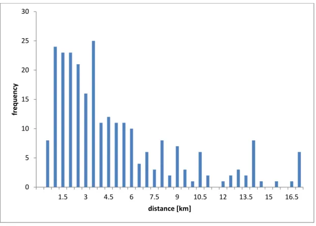
The answers range from 100m to 21km, with the majority of answers pertaining to
shorter trips: the mean of the distance is 4.82 and the median is 3.40 which
indicates positive skewness of the data. The skewness is 1.56 which confirms that
the most answers refer to trips whose lengths fall in the shorter half of the range.
This is made clear when the data is visualised. The histogram representing
frequency with which travel distances were given in the responses to the
questionnaire is presented in Figure 2. The bin width was selected as 0.5km as this
value makes for the most meaningful visualisation. This value is not used in further
30
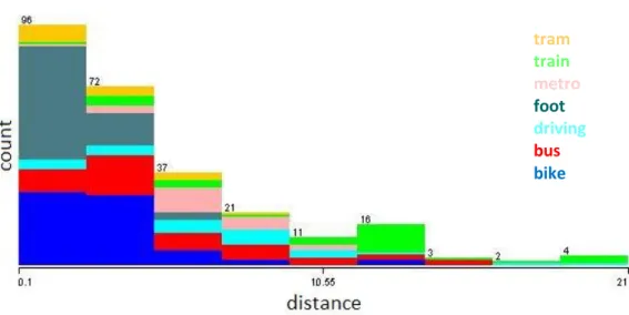
Figure 2 Travel distance histogram.
This indicates that since more data is present in the shortest distances a special
focus should be given to this part of the data range. Further analysis takes that fact
into account and a subset of data is selected for a closer examination. A closer look
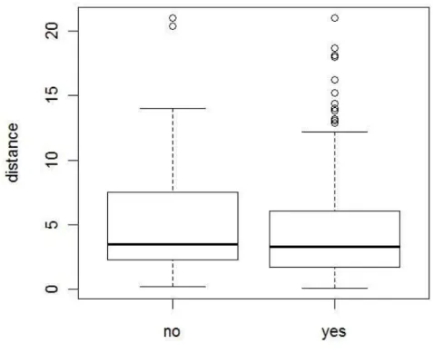
at the data distribution (Figure 3) between the “known” and “unknown” categories
reveals that the “unknown” has a slightly larger range. This is most easily explained by the fact that the best-known routes are the ones that travellers use frequently,
on a daily basis. Longer commutes are typically not as common as shorter ones.
Another reason for this lack of symmetry may be however the questionnaire’s participants’ backgrounds. This is addressed in more detail on page 37 and onwards. Figure 3 also indicates however, that the median distance for both classes is almost
identical, the first two quartiles of answers in both “known” and “unknown”
categories have very similar distribution. This means that for the trips shorter than
the median distance (3.4km) there appears to be little or no bias towards one or the
other category.
0 5 10 15 20 25 30
1.5 3 4.5 6 7.5 9 10.5 12 13.5 15 16.5
fr
e
q
u
e
n
cy
31
Figure 3 Distance against route familiarity box plot
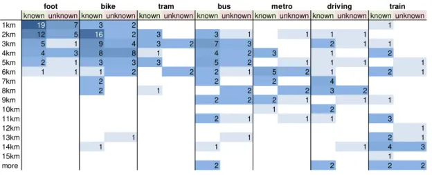
Table 1 presents the summary of questionnaire responses used for initial
exploratory data analysis. The table presents how many answers were given for
journeys by each mean of transport and if the route was previously known to the
traveller. The distance was arbitrarily divided into classes with bin width of one
kilometre. This value is not used in further analysis and is used only for exploratory
32
Table 1 Questionnaire results summary
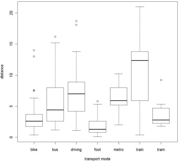
Table 1 demonstrates how certain modes of transport are preferred according to
travel distance. Predictably, walking is most common for short trips under one
kilometre and few people are willing to use public transportation for journeys
shorter than two kilometres. This is clearly visualised in Figure 4 with box plots of
each individual mean of transport. This figure also shows a clear differentiation
between the modes of transport as far as travel distance is concerned.
known unknown known unknown known unknown known unknown known unknown known unknown known unknown
1km 19 7 3 2 1
2km 12 5 16 2 3 3 1 1 1 1
3km 5 1 9 4 3 2 7 3 2 1 1
4km 4 3 8 8 1 4 2 3 1 2
5km 2 1 3 3 3 5 2 1 1 1 1
6km 1 1 1 2 2 2 1 5 2 1 2 1
7km 2 2 2 4
8km 2 1 2 2 3 2
9km 2 2 2 1 1 1
10km 1 2
11km 2 1 1 1 3
12km 1
13km 1 1 2 1
14km 1 1 1 4 3
15km 1
more 2 2 2 2
33
Figure 4 Transport mode dependence on distance box plot.
The proportional usage of all the modes of transport according to distance is
visualised in Figure 5. It makes clear what percentage of trips at a given distance are
34
Figure 5 Breakdown of transport modes according to distance
However, there is no immediately visible difference between journeys made with
prior knowledge of the route versus those where no such knowledge existed.
Overall, out of 262 responses analysed, 179 of them refer to trips where the route
was known beforehand (68%) and 83 refer to trip where the route was not known
(32%). More detailed breakdown is presented in Figure 6. This indicates that most
of the questionnaire participants preferred describing familiar trips – or that it was
easier for them to recall more examples of such trips.
Figure 6 Route knowledge plotted against the route length.
tram train
metro
foot driving bus bike
35 Figure 7 visualises the difference in modes of transport between the trips taken
with prior knowledge of the route versus those taken when no such knowledge
existed and Table 2 presents the data in detail. Together, the figure and the table
indicate that the difference between the trips with “known” and “unknown” routes
– where present – is very small (less than or equal to three percentage points) when
examined for the whole range of distance values. This means that any subsequent
analysis should not be biased towards one or the other.
Figure 7 Unknown (left) and known (right) routes broken down into various modes of transport. Vertical axis normalised for comparison.
bike bus driving foot metro train tram
unknown 27% 18% 8% 22% 10% 11% 5%
known 25% 17% 10% 24% 7% 11% 6%
overall 26% 17% 10% 23% 8% 11% 6%
Table 2 Unknown and known routes broken down into various modes of transport.
Answering the question if the prior knowledge of the route influences the transport
mode choice for a given distance requires a more complex analysis method that
would take into account the whole range of all the analysed variables.
3.4. STATISTICAL ANALYSIS
The aim of the statistical analysis was to find if prior knowledge of the route to be
taken, which implies at least approximate knowledge of the route length (Montello,
tram train
metro
36 2009), influences the choice of mode of transport. Using WEKA, a number of
multilayer perceptron networks as well as logistic regression models have been
built. Furthermore, an additional version of the dataset was created by removing
the “familiar” variable in order to compare estimates and thus judge significance of
this variable. Those models displayed a root relative square error in the range of
77-93%. To try to limit the amount of variables the algorithm should deal with, a
separate models were also built for each of the individual modes of transport to
look for a relationship only between the route familiarity and distance route length.
These models however were characterised by root relative square error exceeding
100%. Such high error values discourage drawing any conclusions from these
models so another method was used.
Using R, a logistical regression model has been built to identify the statistical
significance of route familiarity. The summary of its findings is presented below.
glm(formula = transport ~ distance + as.factor(familiar), family =
binomial(link = "logit"),
na.action = na.pass)
Deviance Residuals:
Min 1Q Median 3Q Max
-2.3744 -1.3681 0.6643 0.8606 1.0508
Coefficients:
Estimate Std. Error z value Pr(>|z|)
(Intercept) 0.27226 0.32015 0.850 0.395103
distance 0.16566 0.04935 3.357 0.000788 ***
as.factor(familiar)yes 0.16581 0.31212 0.531 0.595259
---
Signif. codes: 0 ‘***’ 0.001 ‘**’ 0.01 ‘*’ 0.05 ‘.’ 0.1 ‘ ’ 1
According to the model results route length is a significant factor for mode of
transport choice. This was a conclusion to be expected, demonstrated by the raw
37 The model indicates however that there is no statistically significant effect of prior
route knowledge on transport mode choice by the traveller. Since the hypothesis
posed for this work is disproven, formalisation of this concept as an extension of the
Umwelt model is not justified. However, the model can still be extended by the
concept of functional distance as described on page 42.
3.5. PARTICULAR EXAMPLES AND GEOGRAPHIC VISUALISAT ION
As an additional way of exploratory data analysis two subsets of the data were
selected for geographic visualisation. The Polish Tricity area and Münster are the
most represented in the collected data.
The questionnaire data was geocoded for visualisation using the MapBox script for
Google Docs that looks up WGS84 coordinates for the input search query and
returns them in decimal degrees format using Yahoo!’s or MapQuest’s geocoding service. The Yahoo!’s service proved to return more accurate answers. The result is that next to the existing data columns in the spreadsheet the latitude and longitude
columns are created and populated with coordinates. The table was then exported
to a file and read by ArcToolbox ‘XY to line’ tool that uses startpoint’s and endpoint’s X and Y coordinates to plot straight lines and save the result as a
shapefile. Each line corresponds to one trip. Using an additional ID field and join
command these lines were then annotated with the mode of transport and route
38
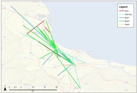
Figure 8 Trips in the Tricity, Poland area.
39 In Figure 8 the following observations can be made. There are two main areas
where most trips origin or destination lie. One of these is Gdańsk’s central
residential area and the other is the city centre. Most of the trips taken along the
axis of the agglomeration were made by suburban train whose tracks go parallel to
the coastline and provide the fastest public transportation method for longer trips.
Perpendicular to this axis are Gdańsk’s tram lines and Gdynia’s bus lines that act as
feeder connections to the train line for longer trips or simply as local connections.
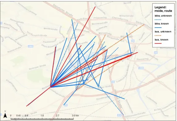
In Figure 9 some points of interest can be clearly identified that correspond to
places frequently visited by questionnaire participants: the University student
residence at Boeselagerstraße 75 and Institute for Geoinformatics (ifgi) facilities at
Weseler Straße 253 and Robert-Koch-Straße. Due to the popularity of bike as a method of transport in Münster there are many of such trips visible for all but the longest distances. Since both the student residence and ifgi are rather outside of
the city centre there are no short (below 1km) trips reported.
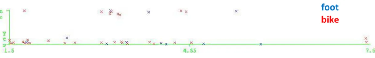
Finally, the data relevant for the Münster area has been plotted (Figure 10) for
another way of visualisation. The higher row in the plot represents unfamiliar
routes and the lower row represents familiar routes. Jitter has been added to the
plot to prevent data points from overlapping.
Figure 10 Münster walking and cycling trips. X axis represents distance, Y axis represents route familiarity.
The same data was also visualised on a map (Figure 11). Trips made on foot were
removed for the sake of clarity. This allowed for creating a legible map where both
means of transport and route familiarity could be represented.